Aquarium: A Comprehensive Framework for Exploring Predator-Prey

Dynamics Through Multi-Agent Reinforcement Learning Algorithms

Michael K

olle

, Yannick Erpelding

, Fabian Ritz

, Thomy Phan

, Steffen Illium

and Claudia Linnhoff-Popien

Institute of Informatics, LMU Munich, Munich, Germany

Thomas Lord Department of Computer Science, University of Southern California, Los Angeles, U.S.A.

Keywords:

Reinforcement Learning, Multi-Agent Systems, Predator-Prey.

Abstract:

Recent advances in Multi-Agent Reinforcement Learning have prompted the modeling of intricate interactions

between agents in simulated environments. In particular, the predator-prey dynamics have captured substantial

interest and various simulations been tailored to unique requirements. To prevent further time-intensive

developments, we introduce Aquarium, a comprehensive Multi-Agent Reinforcement Learning environment

for predator-prey interaction, enabling the study of emergent behavior. Aquarium is open source and

offers a seamless integration of the PettingZoo framework, allowing a quick start with proven algorithm

implementations. It features physics-based agent movement on a two-dimensional, edge-wrapping plane.

The agent-environment interaction (observations, actions, rewards) and the environment settings (agent speed,

prey reproduction, predator starvation, and others) are fully customizable. Besides a resource-efﬁcient

visualization, Aquarium supports to record video ﬁles, providing a visual comprehension of agent behavior. To

demonstrate the environment’s capabilities, we conduct preliminary studies which use PPO to train multiple

prey agents to evade a predator. In accordance to the literature, we ﬁnd Individual Learning to result in worse

performance than Parameter Sharing, which signiﬁcantly improves coordination and sample-efﬁciency.

1 INTRODUCTION

Reinforcement Learning (RL) has emerged as a

pivotal paradigm to train intelligent agents for

sequential decision-making tasks in many domains,

ranging from games, robotics to ﬁnance and

healthcare (Mnih et al., 2015; Silver et al., 2018;

Haarnoja et al., 2019; Vinyals et al., 2019).

The ability of RL agents to learn from interacting

with a problem and adapt their behavior to optimize

for long-term beneﬁt positioned RL as a promising

approach to realize decision-making systems (Sutton

and Barto, 2018). Multi-Agent Reinforcement

Learning (MARL) revolves around the dynamics of

learning in the context of other agents and addresses

scenarios like collaborative robotics, social dilemmas,

and strategic games, where agent interactions are

crucial for success (Albrecht et al., 2023).

Predator-prey domains are widely used to analyze

aspects of agent cooperation, competition, adaptation,

and learning (Diz-Pita and Otero-Espinar, 2021; Li

et al., 2023). Rooted in ecological studies, this

scenario models the interaction between pursuing

predators and evasive prey, allowing to study a wide

range of technical, societal and ecological aspects of

multi agent systems. For example, one line of work

ﬁrst found emergent swarming and foraging behavior

among learning prey agents (Hahn et al., 2019; Hahn

et al., 2020b) and later showed that swarming is

a nash equilibrium under certain conditions (Hahn

et al., 2020a). Subsequently, sustainable behaviour

of single learning predator agents (Ritz et al., 2020)

as well as herding and group hunting of multiple

learning predator agents was achieved (Ritz et al.,

2021). Swarming and group hunting have prevailed

at various places in nature, thus it is highly interesting

to study the emergence of such phenomena among

artiﬁcial agents.

While predator-prey scenarios are common in the

RL community, studies have mostly been conducted

in different environment implementations. Yet,

developing RL environments is time-intensive and

error-prone: abstraction and granularity have to be

balanced, a trade off between simulation precision

and computational speed has to be found, the

choice of algorithm should not be restricted and

Kölle, M., Erpelding, Y., Ritz, F., Phan, T., Illium, S. and Linnhoff-Popien, C.

Aquarium: A Comprehensive Framework for Exploring Predator-Prey Dynamics Through Multi-Agent Reinforcement Learning Algorithms.

DOI: 10.5220/0012382300003636

Paper published under CC license (CC BY-NC-ND 4.0)

In Proceedings of the 16th International Conference on Agents and Artiﬁcial Intelligence (ICAART 2024) - Volume 1, pages 59-70

ISBN: 978-989-758-680-4; ISSN: 2184-433X

reproducibility has to be ensured.

Thus, we present a standardized environment for

future research on predator-prey scenarios (see Fig. 1)

that builds upon the environments used in (Hahn et al.,

2019; Hahn et al., 2020b; Hahn et al., 2020a; Ritz

et al., 2020; Ritz et al., 2021). Our implementation

offers a seamless integration of the PettingZoo

framework (Terry et al., 2021), allowing a quick start

with proven MARL algorithm implementations. As

our implementation is fully customizable, it offers

a ﬂexible and re-usable base to efﬁciently explore

a variety of scenarios, e.g. regarding population

dynamics, social dilemmas, sustainability, and (self-)

organisation. Our contributions are:

1. An overview of predator-prey environments used

in the (MA)RL community.

2. A uniﬁed yet customizable environment that

covers all identiﬁed aspects and is compatible to

the proven MARL algorithm implementations of

the PettingZoo framework.

3. Preliminary experiments reproducing emergent

behaviour of learning agents and demonstrating

the scalability of modern MARL paradigms in our

environment.

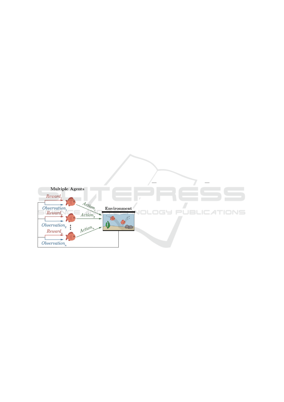
Figure 1: The Multi-Agent Reinforcement Learning

Cycle (c.f. (Zhong-Yu et al., 2010)). Within the

aquarium environment of n agents, each optimizes its

policy to maximize individual rewards, while concurrently

inﬂuencing the observations and rewards of others.

Our work is structured as follows. In the following

Section 2, we describe the predator-prey scenario.

In Section 3, we review existing applications of the

predator-prey scenario to identify all key components

and concepts that are required for thorough studies.

In the subsequent Section 4, we explain how we

incorporated these components and concepts in our

Aquarium environment, which forms the basis of our

experimental framework. In Section 5, we describe

our experimental setup, and then provide and discuss

the according results in Section 6. We conclude in

Section 7 with a summary of key insights, current

limitations and suggestions for future research.

2 PREDATOR-PREY SCENARIO

Population dynamics (biomathematics) study how

single and multiple species coexist and interact in

the same habitat (Diz-Pita and Otero-Espinar, 2021).

Here, the predator-prey scenario models the dynamics

between two types of organisms: predators and prey.

Predators are organisms that hunt and consume other

organisms. Prey are organisms that try to evade and

survive. In nature, some examples are lion and zebra,

fox and rabbit, or shark and ﬁsh.

Independent of each other, Volterra and

Lotka initiated investigations on the ecological

predator-prey scenario in the 1920s (Alfred, 1925;

Volterra, 1926). Both formulated a pair of ﬁrst-order

nonlinear differential equations that describe the

dynamics of predator-prey interactions within an

ecological system. These involve two primary

variables and capture the instantaneous growth rates

of both populations (prey x, predator y):

= α · x − β · x · y and

= δ · x · y − γ · y (1)

where t is the time, α is the prey reproduction rate,

β is the predation rate, δ is the predator reproduction

rate and γ is the predator mortality rate.

The system dynamics are characterized as

follows: when the predator population increases,

this exerts pressure on the prey population, leading

to a decline of available prey. As a result, the

predator population may then also decline due to

reducing food supply. With fewer predators, the

prey population can recover, initiating a new cycle of

population ﬂuctuations, which leads to a balance in

the ecosystem.

Furthermore, the predator-prey relationship

can lead to co-evolution between the two

groups. Through continuous interactions and

adaptations, both populations may undergo reciprocal

evolutionary changes. The prey may develop

defensive mechanisms, such as camouﬂage, warning

signals, or toxins, to deter predation. In response,

the predators may evolve better hunting tactics,

specialized adaptations, or improved sensory

capabilities to overcome these defenses.

Understanding the predator-prey relationship is

essential for conservation efforts and sustainable

management of ecosystems. By studying and

conserving these interactions, scientists, and

ecologists can better understand the elaborate system

of intertwined life dynamics and the delicate balance

ICAART 2024 - 16th International Conference on Agents and Artiﬁcial Intelligence

that sustains natural environments. With increasing

computational resources, predator-prey simulations

have become a common environment for Single-

and Multi-Agent RL algorithms, which has in

fact been advocated 25 years ago (Grafton and

Silva-Echenique, 1997).

3 RELATED WORK

We aim to provide a versatile RL environment with all

key features of previous research. To identify these,

we review applications of (MA-) RL to predator-prey

scenarios in the following.

The ﬁrst aspect is the spatial representation.

Discrete, two-dimensional predator-prey simulations

for multi-agent systems have been around for

more than 20 years (Stone and Veloso, 2000),

sometimes also referred to as pursuit-evasion. In

discrete simulations, agent positions and movement

are restricted to grid cells. Due to their good

scalability, they are often used as a preliminary

test bed for cooperation (Gupta et al., 2017) and

resilience (Phan et al., 2021) in MARL, as well

as to study the dynamics of large populations with

up to a million agents (Yang et al., 2018). The

latter also observed the emergence of Lotka-Volterra

cylces. However, we refrain from modeling discrete

positions as such a coarse spatial representation

prevents meaningful studies on swarming behavior:

this requires precise steering to adjust orientation,

distance and alignment (Reynolds, 1999). To enable

agents to move accordingly, a continuous spatial

model is required.

The next key aspect is the number of dimensions.

Modeling three-dimensions (Berlinger et al., 2021)

comes at the cost of increased mathematical and

conceptual complexity. In fact, a continuous,

two-dimensional, edge-wrapping plane has been

shown shown to be sufﬁcient to study complex agent

interactions: By training prey with the RL algorithms

DQN and DDPG to survive as long as possible, (Hahn

et al., 2019) observed the emergence of ﬂocking

behavior in the presence of predators as described by

(Reynolds, 1987). Follow-up research by (Hahn et al.,

2020a) showed that swarming can be a sub-optimal

Nash equilibrium in predator-prey scenarios and

illustrated how (not) forming a swarm puts the

prey into a social dilemma, demonstrating that two

dimensions are sufﬁcient to explore the complexity

of the interplay between individual and collective

behaviors in swarming dynamics. In a simulation

with similar characteristics, (H

uttenrauch et al., 2019)

propose a MARL variant of the RL algorithm DDPG.

Their agents communicate in local neighborhoods,

e.g. to exchange information about targets to be

localized, and use an efﬁcient representation of local

observations to improve scaling.

Despite a suitable spatial representation, the

aforementioned environments do not consider

collisions and allow agents to overlap, which is

the third key aspect. Missing collisions make it

unnecessary for prey agents to keep distance to each

other and greatly simpliﬁes to escape from predators.

The work of (Ritz et al., 2020) added elastic collisions

and a moment of inertia to the environment of (Hahn

et al., 2019) and trained an RL predator to capture

prey. In a two-phase training approach, the predator

adapted towards a balanced strategy to preserve the

prey population. Subsequently, (Ritz et al., 2021)

found multiple learning predators to learn sustainable

and cooperative behavior amid challenges such as

starvation pressure and a tragedy of the commons.

Environment parameters such as edge-wrapping,

agent speed, or the observation radius to signiﬁcantly

impacted their results.

Another line of research uses a two-dimensional

plane with collision physics and additional

obstacles: (Mordatch and Abbeel, 2018) study

the emergence of communication amongst learning

agents and (Lowe et al., 2017) propose the MARL

algorithm MADDPG, which achieves signiﬁcantly

better results than purely decentralized actor-critic

algorithms. This suggests that communication

and organization are easier to learn centrally when

scenarios require coordination. However, their

environment lacks edge-wrapping. This allows

agents to (theoretically) move to inﬁnity and for

practical reasons, agents need to be stopped from

doing so. Thus, the concept of landmarks to which

agents shall (always) navigate to is used, which limits

the applicability to study swarm behavior.

However, all aforementioned environments

lack one key feature that has received little

attention in simulations so far but could have

signiﬁcant impact on the preys’ formation and the

predators’ hunting: agent Field of View (FOV) (see

Section 4.1.3). This would allow to study the Many

Eyes Hypothesis (Olson Randal S. and Christoph,

2015) with RL.

In summary, a uniﬁed environment should

1. enable continuous agent navigation in a

unbounded 2D plane through edge-wrapping

similar to (Hahn et al., 2019),

2. use a thorough physics model, e.g. with a

moment of inertia and collisions between agents

and obstacles, similar to (Lowe et al., 2017; Ritz

et al., 2020),

Aquarium: A Comprehensive Framework for Exploring Predator-Prey Dynamics Through Multi-Agent Reinforcement Learning Algorithms

3. allow a ﬂexible environment parameterization

similar to (Ritz et al., 2021) and

4. model agent FOV.

We realize all these key aspects in our Aquarium

environment, which we describe in the following.

4 AQUARIUM

We introduce Aquarium, a comprehensive and

ﬂexible environment for MARL research in

predator-prey scenarios. By making key parameters

accessible, we support for the examination of a

wide array of research questions. Our goal is to

eliminate the necessity for researchers to rebuild

basic dynamics, which is often a signiﬁcantly

time-consuming task, thereby affording more

opportunities for the methodical analysis of relevant

factors. Moreover, employing a uniﬁed simulation

platform eases the reproduction of previous results

and strengthens the reliability of performance

comparisons between different methodologies via a

stable foundation. To include the collective effort

put into existing RL libraries, we implement the

PettingZoo interface (Terry et al., 2021), which

enables out-of-the-box support for CleanRL,

Tianshou, Ray RLlib, LangChain, Stable-Baselines3,

and others. The project is open-source, distributed

under the MIT license, and available as a package on

PyPI

4.1 Dynamics and Perception

The agents in our environment traverse a continuous

two-dimensional toroidal space, enabling seamless

movement across its boundaries (Fig. 2a). Detailed

computations for this toroidal conﬁguration are

explored in the following sections.

The environment supports multiple instances of

two agent types: prey, visually represented as

ﬁsh, and predators, visually represented as sharks.

The actual position of agents is marked by central

point within these representations. Prey agents can

replicate after a speciﬁed survival duration, with the

process capped upon reaching a predeﬁned maximum

prey count. An episode terminates either after a

predetermined number of time steps or when all

agents of one type are eliminated, with predators

also susceptible to starvation after a set number of

unsuccessful hunting steps. Agents are characterized

by attributes like mass, position, velocity, and

acceleration, and utilize essential vectors, namely

https://github.com/michaelkoelle/marl-aquarium

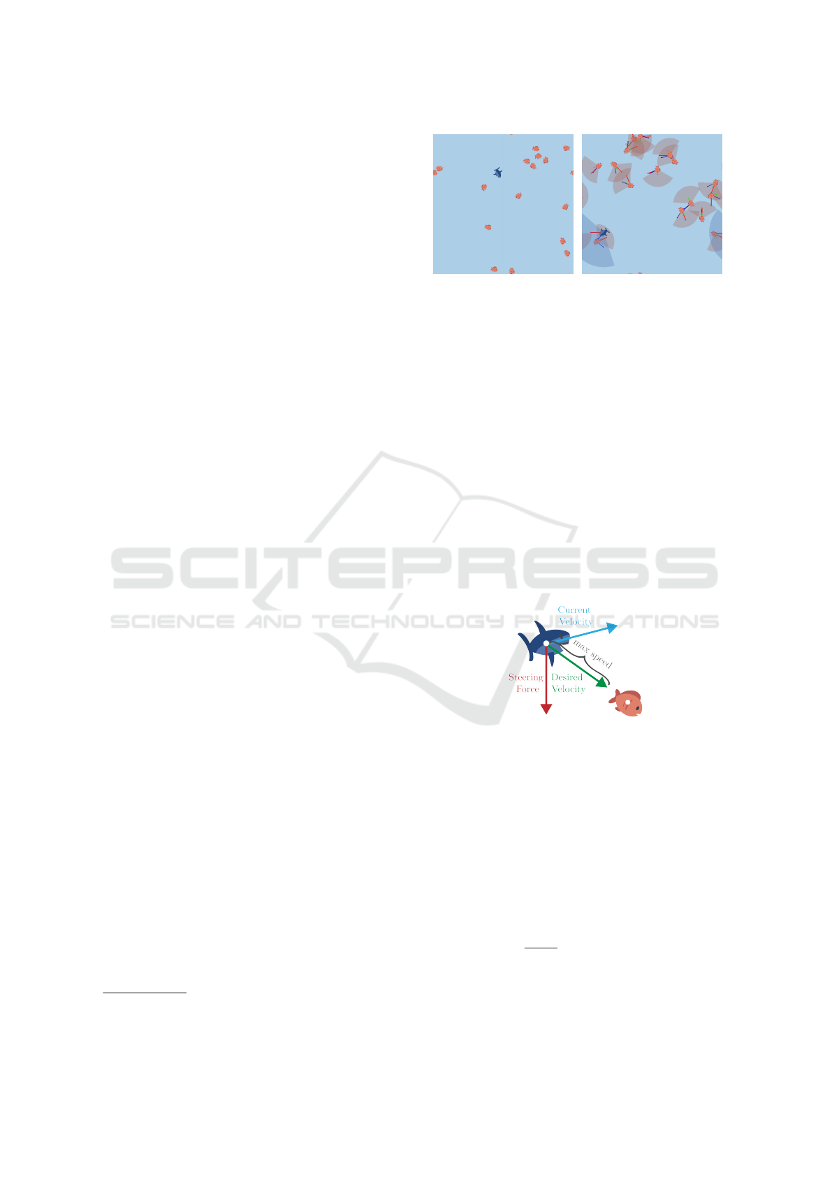
(a) Simple Visualization. (b) Visualization Including

Force Vectors and Cones.

Figure 2: Examples of the Aquarium With 16 Prey (Fishes)

and One Predator (Shark) Agent.

position, velocity, and acceleration vectors, for

navigation.

4.1.1 Movement

In the context of a predator-prey scenario, an agent’s

primary objective involves initiating a directional

movement, which necessitates the manipulation of

its velocity through the application of forces. At

each time step, a steering mechanism, derived from

the algorithm of (Reynolds, 1999), is employed to

guide the agent towards a designated position within

the environment (Fig. 3). This adaptation aligns the

agent, for instance, a predator, and its velocity is

radially aligned towards its designated target, a prey.

Figure 3: Calculation of the Steering Force. A limited

fraction of the steering force is applied to smoothly

transition from the current to the desired velocity, which is

capped by the agent’s maximum speed.

The desired velocity D, a vector pointing from

the agent to the target, is constrained in magnitude

by the agent’s maximum attainable speed s ∈ R. The

steering vector F is the difference between the desired

velocity D and the agent’s current velocity V and is

limited by the agent’s maximum steering force f ∈ R

(Eq. 2).

F =

(

D −V if kD −V k ≤ f

D−V

kD−V k

· f otherwise

(2)

After the calculation of the steering force, the

agent’s new acceleration vector A

is calculated using

the agent’s current acceleration vector A, the steering

ICAART 2024 - 16th International Conference on Agents and Artiﬁcial Intelligence

force F, the agent’s mass m ∈ N, and the maximum

magnitude k ∈ R of the ﬁnal acceleration vector

(Eq. 3).

A +

kA +

· k, (3)

The new acceleration vector A

is then added to

the agent’s current velocity vector V to compute the

new velocity vector V

, which is then limited by the

agent’s maximum speed s.

(

V + A

if kV + A

k ≤ s

V +A

kV +A

· s otherwise

(4)

To ultimately change the agent’s position, the new

velocity vector V

is added to the agent’s position

vector P (Eq. 5).

= P +V

(5)

To increase the ﬂexibility of the environment, the

maximum magnitudes of the desired velocity s, the

steering force f , and the acceleration vector k can be

manipulated, independently of the agent type.

4.1.2 Collisions

As a predator-prey setting consists of predators trying

to capture their prey, interactions between agents are

enabled in this environment. Every agent is equipped

with a circular hitbox of a predetermined radius r ∈

R around the agent’s center. Detecting collisions

between two agents A and B involves calculating the

distance between them using their positional vectors

and P

. If the computed distance d is smaller than

the the sum of the radii of both agents, i.e. d < r

agents A and B have collided.

When a predator collides with a prey, the prey

is considered captured and can be immediately

respawned at a random position within the

environment if conﬁgured. This ensures a constant

number of prey throughout the entire episode. On

the other hand, if two agents of the same type collide

with each other, they bounce back in the opposite

directions of the other agent. Following a collision,

the new velocity V

of agent A is calculated using its

current velocity V

and the positional vectors of both

agents A and B (Eq. 6). The new velocity V

of agent

B is determined analogously.

= V

− P

(6)

4.1.3 Vision

In an agent-based system, the actions of an agent

are inﬂuenced by the information it perceives from

its environment. Therefore, it is crucial to precisely

deﬁne what the agent can see. In the default setup of

this environment, each agent has complete visibility

of all other agents, implying that it knows the exact

positions of every agent. However, for a more realistic

simulation, we can impose restrictions on the agent’s

view, rendering the environment partially observed. A

widely-used approach involves establishing a limited

viewing distance, and thus creating a circular vision

ﬁeld around the agent. Consequently, the agent

can only perceive other agents situated within this

predetermined viewing distance.

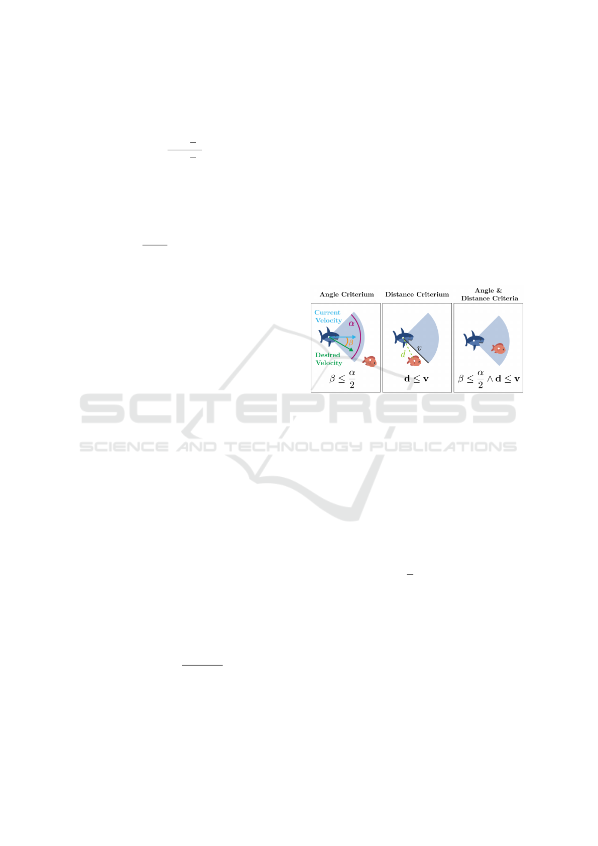
Figure 4: Angle and Distance Criteria. An agent is

considered within the ﬁeld of view only if both conditions

are met: staying within a deﬁned angular range, α (left),

and not exceeding a speciﬁed distance, v (middle). Both

conditions are fulﬁlled (right).

To further reﬁne the agent’s perception, we

introduce a restriction, known as the FOV constraint,

within the agent’s frontal direction (Fig. 2b). This

entails that an agent A is only capable of seeing

other agents positioned within a speciﬁc angular

range α in front of it, at a deﬁned distance. As

illustrated in Fig. 4, the determination of an agent’s

inclusion within its FOV involves fulﬁlling two

speciﬁc conditions (Eq. 7).

β ≤

∧ d ≤ v (7)

Firstly, the angle β formed between the agent’s

current velocity vector V and the desired velocity

D must be smaller than α. Secondly, the distance

d separating the two agents must be shorter than

the agent’s designated viewing distance v. To

account for agents wrapping around the boundaries,

the FOV is duplicated eight times, each instance

situated at distinct locations, as depicted in Fig. 5a.

Note that this approach may not be the most

efﬁcient approach and there remains the potential

for future enhancements. The values for the agent’s

designated viewing distance v and FOV angle α can

Aquarium: A Comprehensive Framework for Exploring Predator-Prey Dynamics Through Multi-Agent Reinforcement Learning Algorithms

be independently adjusted for each agent type in this

environment.

(a) Field of View. (b) Distances Between

Agents.

Figure 5: Distance and Field of View Calculation in a Torus.

4.1.4 Distance

In a toroidal environment, determining the shortest

distance between two positions becomes intricate due

to the multiple boundary-crossing paths. Unlike a

bounded two-dimensional plane, which has a singular

distance between points, a torus offers numerous

direct paths, some of which may be shorter than

conventional distances, as depicted in Fig. 5b. Our

primary objective is to ﬁnd the shortest of these paths.

Instead of computing all potential distances and

choosing the smallest, we initially assess the standard

Euclidean distance within screen space, followed by

conditional adjustments based on the environment’s

width (W ∈ N) and height (H ∈ N). Thus, the distance

d between two positions A and B can be calculated as:

d(A, B) =

min(|x

− x

|,W − |x

− x

min(|y

− y

|, H − |y

− y

(8)

4.1.5 Direction Vector

To obtain the direction from one point to another in

the form of a vector, we introduce two points, A and

B, representing the initial position and destination.

Additionally, let W ∈ N and H ∈ N be the width and

height of the environment. The directional vector is

required for the heuristics described in Section 5.2.

We deﬁne the directional vector D with D(A, B) =

, y

), where

(

− x

, if |x

− x

| >

− x

, otherwise

where

(

− y

, if |y

− y

| >

− y

, otherwise

(9)

4.2 Agent-Environment Interaction

In our modeled ecosystem, the relationship

between agents and their environment is crucial

for comprehending and inﬂuencing predator-prey

interactions. Utilizing the Markov Decision Processes

framework, we divide the agent behaviors into three

key components: observations, actions, and rewards,

each of which will be elaborated in the following

subsections. It is imperative to note that since our

environment operates in a deterministic manner, all

transition probabilities are equal to one.

4.2.1 Observations

The environment is partially observable and therefore

observations constitute only a subset of the overall

state of the environment. Both types of agents

can possess different observation spaces that can be

manipulated through varying conﬁgurations. The

environment offers the ﬂexibility to use an FOV

mechanism characterized by predeﬁned parameters

encompassing view distance and angle, as described

in Section 4.1.3. Furthermore, a restriction

can be imposed on the number of neighboring

agents that an agent can perceive. For instance,

predators can be restricted to perceive a maximum

of three prey agents. Through this modular

approach to managing agent observations, the

environment provides maximal customizability and

reduces coupling between components, enabling the

simulations to be more readily adapted to novel

research needs.

Under the standard observation conﬁguration,

an observing agent o receives a 6-tuple of each

neighboring agent e, encompassing the neighboring

agent’s type, position, distance, orientation, and

speed (Fig. 6). The position is represented

in terms of polar coordinates relative to the

observer, whereas distance, orientation, and speed are

characterized by continuous numerical values. Given

the environment’s toroidal structure, the shortest

euclidean distance to the neighboring agent is taken,

as described in Section 4.1.4. An agent’s orientation

is quantiﬁed in degrees within the range of [0

◦

, 360

◦

while the speed is constrained by the maximum speed

an agent can have.

Consequently, each observer receives this

observation tuple for itself and the b nearest

neighboring agents with b representing the upper

limit of perceivable neighboring agents. All

information is encapsulated within an ordered vector

of constant length, restricted by the value of b, and

within which the b neighbors are ordered based on

their respective distance. In scenarios, where an

ICAART 2024 - 16th International Conference on Agents and Artiﬁcial Intelligence

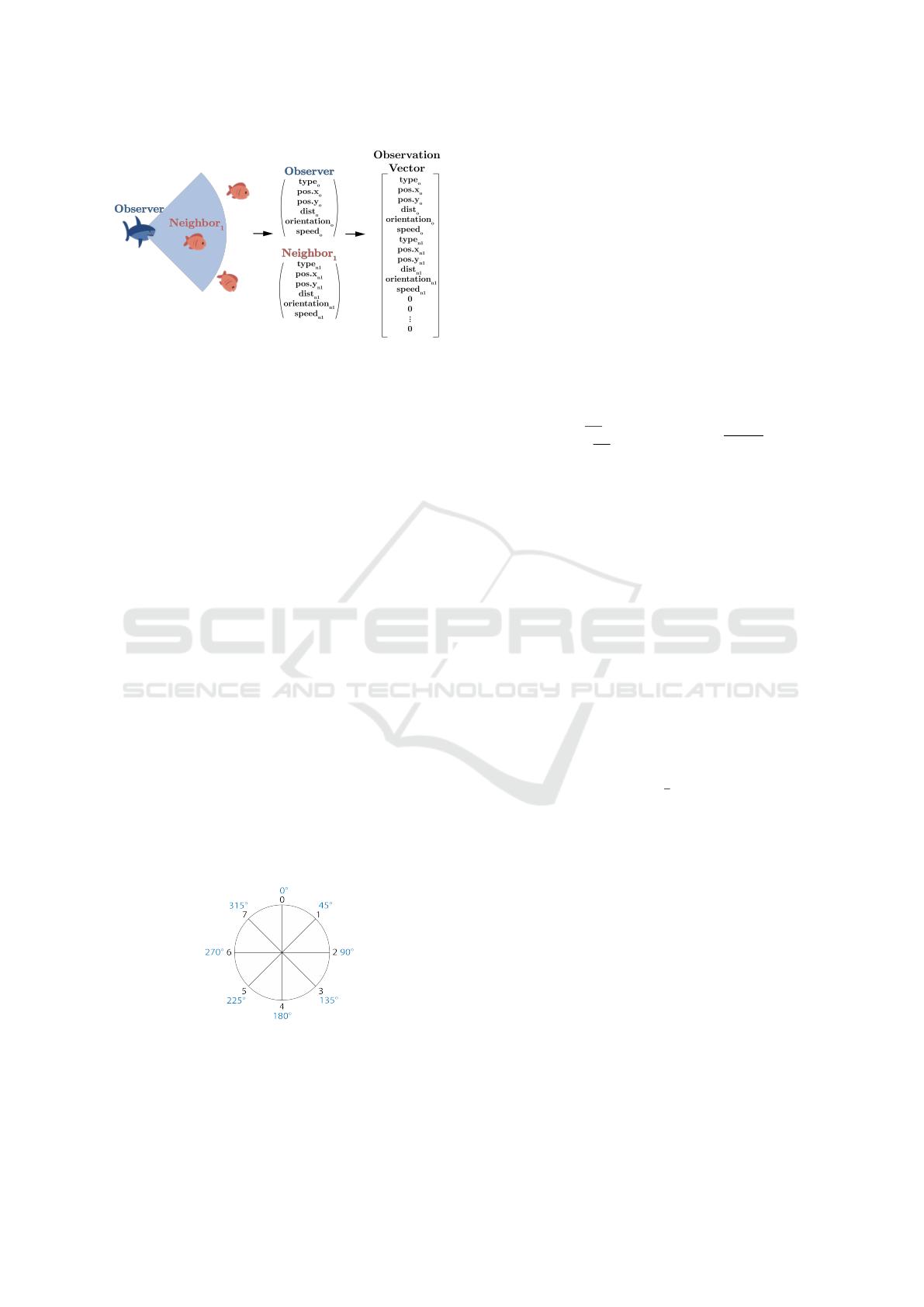
Figure 6: Construction of the Observation Vector. The

observation vector is an ordered vector containing 6-tuples

for the observer and the b nearest neighboring agents, with

b designating the upper limit of observable neighboring

agents.

agent’s perceptual ﬁeld yields fewer neighboring

agents than the deﬁned maximum b, the vector length

is preserved by zero padding. Subsequently, this

vector undergoes a rescaling procedure to ﬁt within

a range spanning from 0 to 1 or alternatively, -1 to

1, depending on the context. This transformation

into a vectorized format empowers the interpretation

of observations by the RL algorithm, enhancing its

ability to process the information effectively.

4.2.2 Actions

The environment uses distinct modular functions

to execute agent actions. This facilitates the

customization of independent action spaces for

both predators and prey, aligning with the speciﬁc

requirements of research objectives. In pursuit

of broad applicability, the action space within the

environment is designed to be compatible with

a variety of agent models, including machine

learning algorithms, random actions, and static

algorithms. Regardless of the speciﬁc control logic,

all agents share the same deﬁned action space,

delineating the permissible movement options within

the environment.

Figure 7: Illustration of the Action Space. Agents select

actions from a discrete set of integers, each representing

a speciﬁc direction. For example, in this 8-option action

space, choosing 2 indicates an intent to move east.

Within this environment, a discrete action space

is utilized, wherein action choices are encoded as

integers that correspond to particular directional

movements that agents can solicit. For instance, if the

action space encompasses eight possible choices, as

depicted in Fig. 7, an action a of value 0 symbolizes

an intention to advance northward, while a value

of 1 could denote a northeastern movement, and so

forth. These designated directions are subsequently

translated into degrees to calculate the desired

velocity that dictates the intended agent movement.

To turn an action a from an agent’s model into an

angle of degrees γ, Eq. 10 is applied, with n being

the number of actions and desired velocity vector D is

then calculated accordingly.

D =



sin(γ ·

180

)

−cos(γ ·

180

)



where γ =

360 · a

(10)

The method by which the desired velocity

inﬂuences the agent’s movement is detailed in

Section 4.1.1.

4.2.3 Rewards

Rewards serve as the primary feedback signal

enabling RL algorithms to improve agents’ policies.

In our conﬁguration, the predator agent receives

solely a predeﬁned reward for catching a prey agent,

modeling the goal of hunting success. Every other

state is classiﬁed as neutral, providing neither reward

nor punishment, which ensures that no behavioral

bias is introduced. In environments featuring multiple

predators, the predeﬁned reward r received upon

catching a prey can be divided. When there are n

predators located within a shared catch zone of a

predetermined radius from the prey location, each

predator receives a reward of

The goal of the prey is to not collide with a

predator and to survive as long as possible. For

this, they receive a positive predetermined reward for

each time step survived and another negative speciﬁed

reward for the collision with a predator which ends

their life.

The reward structure for the predator agents was

adapted from (Ritz et al., 2021), while the reward

structure for the prey agents was inspired by the

concepts introduced by (Hahn et al., 2019). While

the existing setup of the environment relies on

these predetermined reward frameworks, it’s worth

noting that the environment incorporates modular

functionalities that enable easy modiﬁcations to the

established reward system.

Aquarium: A Comprehensive Framework for Exploring Predator-Prey Dynamics Through Multi-Agent Reinforcement Learning Algorithms

4.3 Limitations

Despite the environment’s adaptability to a variety

of scenarios, we sacriﬁce generality in favor

of simplicity by using a two-dimensional plane.

This limits the scope of applications: in nature,

predator-prey interactions generally occur in a

three-dimensional context. Also, most UAV scenarios

require a third degree of freedom (altitude). During

the time of writing, the environment lacks metrics for

cohesion, ﬂocking, and other collective phenomena

inherent to predator-prey settings, which we plan to

add in future releases. Also, the environment size is

bound by the simulation efﬁciency, which we plan to

improve by optimizing vector operations and the FOV

mechanic.

5 EXPERIMENTAL SETUP

We demonstrate the potential of the Aquarium

environment as a suitable predator-prey scenario for

MARL by resembling typical research setups found

in related work. We follow the experimental setup

of (Hahn et al., 2019), where multiple prey are

trained with RL to escape a predator that is guided

by a heuristic called NaivChase. Aquarium used

the default values for all parameters which can be

found in the provided repository. In the following,

we describe how we train the prey, which baselines

we use and which metrics we choose to evaluate the

performance.

5.1 RL Algorithm

We train our prey agents with the RL algorithm

Proximal Policy Optimization (PPO) (Schulman

et al., 2017) using the Generalized Advantage

Estimation (GAE). The hyper-parameters are outlined

in Table 1. We conducted two experiments using an

identical parameterization for environment and RL

algorithm. In the ﬁrst experiment, we use the MARL

paradigm Individual Learning (IL) to train the prey

agents (de Witt et al., 2020). Here, each agent trains

an individual policy with its own experiences. In

the second experiment, we use Parameter Sharing

(PS). Here, all agents share the parameters of one

policy. Hence, the prey agents learn from experience

collected collectively. For this experiment, the batch

size was proportionally reduced by dividing it by

the count of agents. For IL and PS, training was

performed for 4000 episodes, each lasting 3000 time

steps with ﬁve different seeds.

Table 1: PPO Hyper-Parameters. These hyper-parameters

were used for training the prey agents in an environment

including a single predator agent.

Parameter Data Type Value

Discount Factor Float 0.99

Batch Size Integer 2048

Clipping Range Float 0.1

GAE Lambda Float 0.95

Entropy Weight Float 0.001

Actor Alpha Float 0.001

Critic Alpha Float 0.003

5.2 Baselines

To asses the trained RL policies, we implemented

several heuristic baselines.

The Random heuristic operates by selecting

actions in an arbitrary manner, devoid of any strategic

consideration or learning process. This represents an

untrained agent and any training should result in a

signiﬁcant improvement.

The Static heuristic is a different set of rules for

predator and prey agents. In case of prey agents,

the heuristic applies the rules of the TurnAway

algorithm reported by (Hahn et al., 2019), where

agents turn 180° away from the predator. This

involves computing the directional vector from the

prey to the predator (see Section 4.1.5), inverting it

and converting it into an angle. Then, this angle is

mapped to an action within the action space (Fig. 7).

In case of predator agents, the heuristic applies the

rules of the NaivChase algorithm reported by (Hahn

et al., 2019). It determines the direction vector from

the predator to the closest prey and converts it into an

action. If a predator has multiple prey within its FOV,

it arbitrarily selects one prey to pursue at each time

step, modelling confusion.

5.3 Metrics

To measure the learning success and analyze the

population dynamics, our framework provides two

pivotal metrics.

Rewards is the undiscounted sum of all rewards

collected per episode. This metric measures how well

an agent is doing on the long run. It does not have

to be normalized since the episode length is constant.

Predator agents are rewarded for capturing prey and

prey agents are rewarded for surviving, Higher values

indicate better performance.

Captures is the sum of captured prey per episode.

It measures the success of predators agents catching

prey (from this point of view, higher values are better)

and the success of prey agents evading the predators

ICAART 2024 - 16th International Conference on Agents and Artiﬁcial Intelligence

(from this point of view, lower values are better). Prey

agents reappear after being caught to keep the episode

length constant.

6 RESULTS

The following section encompasses the outcomes

of the two experiments elucidated in Section 5.1.

Initially, the efﬁcacy of the training approach

wherein individual agents possess distinct policies

is juxtaposed with the baseline models described in

Section 6.1. Subsequently, a comparison between

the two experiments employing distinct training

strategies is presented in Section 6.2. The trained

policies were executed across 200 episodes, each

consisting of 3000 time steps, using ﬁve distinct

seeds in an environment featuring a single predator

governed by the NaivChase heuristic. The same

protocol was followed for the baseline models.

During these runs, both undiscounted rewards and

captures per episode were collected for each prey

agent to compare the different models on their

evading performance. The results of the different

seeds were summarized by averaging the respective

metrics.

6.1 Individual Learning

To recapitulate, each prey agent developed its own

distinct policy through dedicated training, ensuring

that their policy’s learning process exclusively

derived from their unique set of experiences. Our

aim is to replicate the ﬁndings observed in the

study conducted by (Hahn et al., 2019). While

we did not integrate a speciﬁc metric to assess the

extent of prey cooperation, such as swarming, we

anticipate discovering that the ﬁsh learn to enhance

their survival by maintaining a distance from the

predator. Nevertheless, we do not anticipate the

prey agent to embrace the action of executing a 180

◦

turn away from the predator, as performed by the

TurnAway heuristic.

First, we examined the rewards and capture per

episode during the training process. Initially, the

policy’s average rewards, calculated over all prey

agents, closely align with that of the random policy,

as illustrated in Fig. 8. Subsequently, there is a

rapid growth in reward, and after approximately 2000

episodes the increase becomes gradual. The standard

deviation reveals a pronounced dispersion of rewards

across the entire training.

Upon examining the captures per episode, a

similar trend becomes apparent. Initially, the

Figure 8: Average Reward per Prey Agent Using the

Individual Training Strategy. Training was performed for

4000 episodes, each lasting 3000 time steps. The prey

agents were individually trained, such that each agent is

equipped with its unique policy and exclusively learns from

its own experiences. The individual rewards over the six

prey agents were averaged for each episode and the standard

deviation was calculated. The red dotted line represents

the average reward achieved overall episodes with random

behavior.

policy’s capture outcomes closely resemble those

of the random policy. Nonetheless, these captures

undergo a substantial decline until around episode

2000. After this point, the capture rate demonstrates

only a slight additional reduction. Once more,

the standard deviation exhibits notable elevation,

suggesting considerable variability across episodes

regarding the frequency of prey capture events by the

predator.

When comparing the behavior of the prey

agents using the learned policies to the behavior

of those being based on two baselines model,

observed across a span of 200 episodes, it

becomes evident that the TurnAway heuristic has

pronounced effectiveness, yielding notably higher

average rewards in comparison to both the random

and trained prey models. Nonetheless, it is imperative

to acknowledge that the trained policy consistently

maintains superior performance over the random

policy in relation to the speciﬁed reward metric.

Upon evaluating the captures per episode across

the three models, the prey subjected to the trained

policy exhibited an average capture frequency of

approximately ﬁve times per episode (Fig. 9). In

contrast, the prey, under the inﬂuence of the static

algorithm, experienced a notably lower capture rate,

with fewer than one capture per episode on average.

This underscores the effectiveness of the static

algorithm in countering the predator with similar

control.

The trained prey agents exhibited a slight

tendency to move in a direction opposite to that

Aquarium: A Comprehensive Framework for Exploring Predator-Prey Dynamics Through Multi-Agent Reinforcement Learning Algorithms

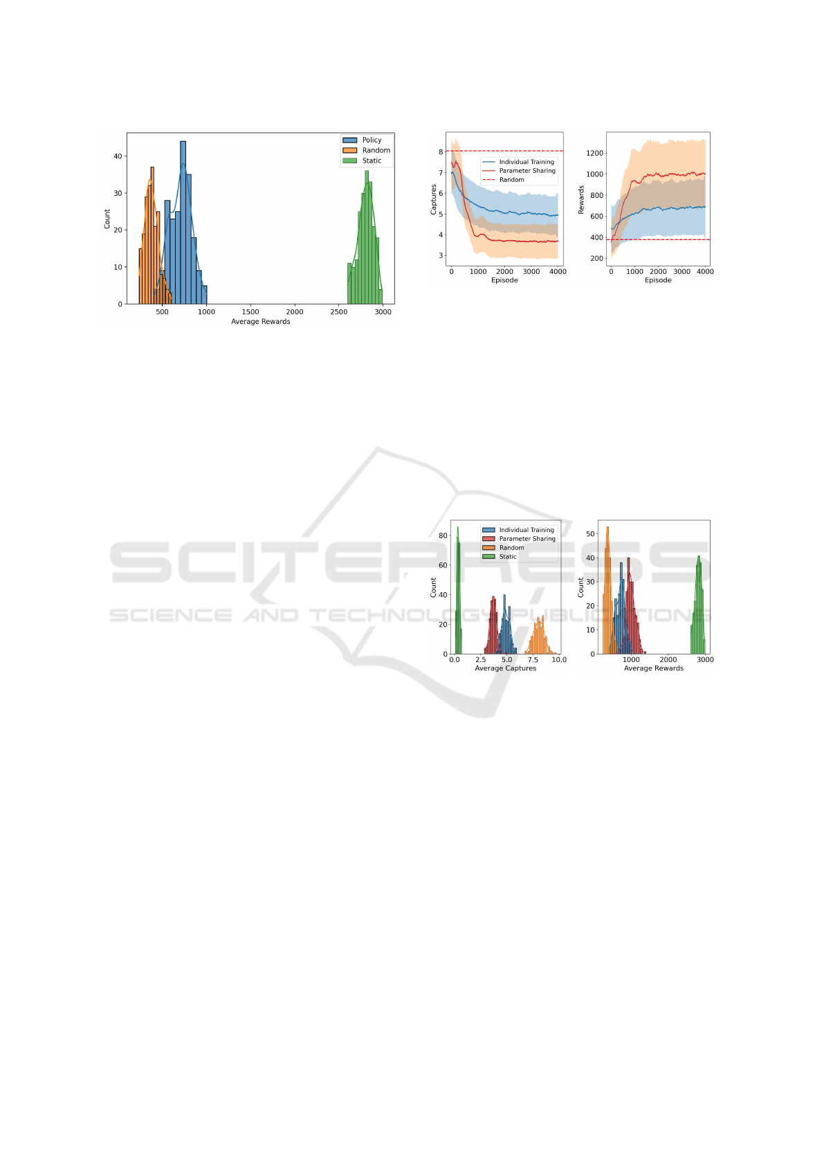
Figure 9: Distribution of the preys’ average rewards in a

scenario with one predator. We compared the trained RL

prey agent (blue) against the Random heuristic (orange) and

the TurnAway heuristic (green) across ﬁve differnent seeds.

of the predator. However, their effectiveness in

executing this evasion behavior remained limited, as

they persisted in directly engaging in actions aimed

at the predator. This choice of action resulted in a

substantial number of captures for the prey, indicating

that the evasion strategy is not highly successful in

preventing capture incidents.

Overall, the prey agents individually trained using

the PPO technique exhibit a marginal improvement

over random movement patterns. However, their

performance remained notably inferior when

contrasted with the efﬁcacy demonstrated by the

TurnAway heuristic. This observation aligns closely

with the ﬁndings of (Hahn et al., 2019), albeit

with the distinction that a more comprehensive set

of metrics is required to comprehensively assess

complex behaviors such as swarming.

6.2 Parameter Sharing

Utilizing parameter sharing among prey agents, as

discussed in Section 5.1, means that each agent

beneﬁts from the collective experiences of the

group, learning from a single policy source. This

approach is expected to accelerate the learning rate,

potentially leading to cooperative behaviors or swarm

formations, confusing the predator ((Hahn et al.,

2019)). Our preliminary results suggest enhanced

survival rates for prey, as they strategically maintain

distance from predators, indicated by the rapid

decline in captures per episode (Fig. 10a) and the

parallel increase in rewards (Fig. 10b).

Additionally, the prey employing the parameter

sharing approach demonstrate markedly improved

post-training performance, aligning with our initial

anticipation of accelerated learning. The prey

subjected to parameter sharing training outperform

(a) Average Captures Over

Prey Agents.

(b) Average Rewards Over

Prey Agents.

Figure 10: Average captures and rewards per prey agent.

We compare individual learning (blue) against parameter

sharing (red). Training was performed for 4000 episodes,

each lasting 3000 time steps. The metrics are averaged over

six prey agents and ﬁve distinct seeds per episode. The

shaded areas represent the respective standard deviation.

the random agents, exhibiting reduced capture rates

and superior rewards compared to the individually

trained prey (Fig. 11). Nevertheless, the performance

of prey governed by the TurnAway heuristic still

surpasses that of the other models.

(a) Average Captures Over

Prey Agents.

(b) Average Rewards Over

Prey Agents.

Figure 11: Distributions of the Average Captures and

Rewards Comparing Both Training Strategies. The

trained policies, individual training (blue) and training

with parameter sharing, the random heuristic (orange), and

the TurnAway heuristic (green) were executed across 200

episodes, each consisting of 3000 time steps, using ﬁve

distinct seeds in an environment featuring a single predator

governed by the NaivChase heuristic.

Upon examining the recorded video of one

episode of the environment consisting of prey agents

trained using parameter sharing, we noticed that the

policy guides all agents to consistently swim in the

same direction. The progress of this phenomenon

becomes evident during training. Fig. 12 showcases

ﬁve distinct images captured at various time steps

throughout the training process. This observation

was unexpected, as this straightforward behavior of

maintaining uniform direction appears primitive in

ICAART 2024 - 16th International Conference on Agents and Artiﬁcial Intelligence

attempting to evade the predator. However, it can

be deduced that the PPO algorithm converged to a

local optimum. Remarkably, this aligns with the

adoption of the alignment rule of swarm behavior,

as elucidated in (Reynolds, 1987), which ultimately

granted them an advantage over the individually

trained, self-centered prey agents.

Figure 12: Illustration of Directional Movement Evolution

of Prey Agents Using Training With Parameter Sharing.

Training was performed for 600 episodes, each lasting 3000

time steps. A single policy was trained collectively based on

the observations of all prey agents. To illustrate the behavior

of the prey agents, ﬁve screenshots at an interval of 100

episodes were recorded.

7 CONCLUSION

In this work, we introduced Aquarium, a

comprehensive and ﬂexible MARL environment

that models predator-prey interaction. By providing

an overview of existing predator-prey environments,

we identiﬁed key aspects required by the (MA)RL

community. Based on that, we provide a customizable

implementation that covers all identiﬁed aspects and

is compatible to the proven MARL algorithm

implementations of the PettingZoo framework (Terry

et al., 2021). In preliminary experiments, we

reproduced emergent behaviour of learning agents

and demonstrated the scalability of modern MARL

paradigms in our environment.

Future prospects can be divided into

three categories: improving the environment

implementation, adding further features and

conducting comprehensive experiments. Regarding

the environment implementation, we hope to reduce

the computational footprint in various aspects, such

as optimizing vector operations and streamlining

computations required for the utilization of the

FOV mechanism. In particular, the integration of

ray tracing techniques (Kuchkuda, 1988) has the

potential to substantially improve performance. We

believe that the pivotal expansion of the environment

to accommodate a larger number of agents is

imperative for the in-depth analysis of swarm

behavior. Regarding additional features, we plan to

add vector ﬂow ﬁelds (Reynolds, 1999) that simulate

water ﬂow or wind. This would allow to investigate

how agents behave in presence of external forces.

Regarding experiments, we plan to replicate group

hunting as reported by (Ritz et al., 2021) and explore

the (optional) FOV mechanism, e.g. to test the Many

Eye Hypothesis (Olson Randal S. and Christoph,

2015) which has not received much attention yet.

Ultimately, we hope for the community to adopt our

environment and provide feedback on deﬁciencies

we may have overlooked.

ACKNOWLEDGEMENTS

This work is part of the Munich Quantum Valley,

which is supported by the Bavarian state government

with funds from the Hightech Agenda Bayern Plus.

REFERENCES

Albrecht, S. V., Christianos, F., and Sch

afer, L. (2023).

Multi-Agent Reinforcement Learning: Foundations

and Modern Approaches. MIT Press.

Alfred, L. (1925). Elements of Physical Biology. Nature,

116(2917):461–461.

Berlinger, F., Gauci, M., and Nagpal, R. (2021). Implicit

coordination for 3d underwater collective behaviors

in a ﬁsh-inspired robot swarm. Science Robotics,

6(50):eabd8668.

de Witt, C. S., Gupta, T., Makoviichuk, D., Makoviychuk,

V., Torr, P. H. S., Sun, M., and Whiteson, S.

(2020). Is independent learning all you need in

the starcraft multi-agent challenge? arxiv preprint,

abs/2011.09533.

Diz-Pita, E. and Otero-Espinar, M. V. (2021).

Predator–Prey Models: A Review of Some Recent

Advances. Mathematics, 9(15):1783.

Grafton, R. Q. and Silva-Echenique, J. (1997). How

to Manage Nature? Strategies, Predator-Prey

Models, and Chaos. Marine Resource Economics,

12(2):127–143.

Gupta, J. K., Egorov, M., and Kochenderfer, M.

(2017). Cooperative multi-agent control using deep

reinforcement learning. In Autonomous Agents

and Multiagent Systems, pages 66–83. Springer

International.

Haarnoja, T., Ha, S., Zhou, A., Tan, J., Tucker, G.,

and Levine, S. (2019). Learning to walk via deep

reinforcement learning.

Hahn, C., Phan, T., Feld, S., Roch, C., Ritz, F., Sedlmeier,

A., Gabor, T., and Linnhoff-Popien, C. (2020a).

Nash equilibria in multi-agent swarms. In ICAART:

Proceedings of the 12th International Conference on

Agents and Artiﬁcial Intelligence, pages 234–241.

Hahn, C., Phan, T., Gabor, T., Belzner, L., and

Linnhoff-Popien, C. (2019). Emergent Escape-based

Aquarium: A Comprehensive Framework for Exploring Predator-Prey Dynamics Through Multi-Agent Reinforcement Learning Algorithms

Flocking Behavior using Multi-Agent Reinforcement

Learning. In Proceedings of the 2019 Conference on

Artiﬁcial Life, pages 598–605.

Hahn, C., Ritz, F., Wikidal, P., Phan, T., Gabor, T., and

Linnhoff-Popien, C. (2020b). Foraging swarms using

multi-agent reinforcement learning. In Proceedings

of the 2020 Conference on Artiﬁcial Life, pages

333–340.

uttenrauch, M.,

c, A., and Neumann, G. (2019). Deep

reinforcement learning for swarm systems. Journal of

Machine Learning Research, 20(54):1–31.

Kuchkuda, R. (1988). An Introduction to Ray Tracing.

Theoretical Foundations of Computer Graphics and

CAD, pages 1039–1060.

Li, J., Li, L., and Zhao, S. (2023). Predator–prey survival

pressure is sufﬁcient to evolve swarming behaviors.

New Journal of Physics, 25(9):092001.

Lowe, R., WU, Y., Tamar, A., Harb, J., Pieter Abbeel,

O., and Mordatch, I. (2017). Multi-agent actor-critic

for mixed cooperative-competitive environments. In

Advances in Neural Information Processing Systems

(NeurIPS), volume 30, pages 6379–6390.

Mnih, V., Kavukcuoglu, K., Silver, D., Rusu, A. A.,

Veness, J., Bellemare, M. G., Graves, A., Riedmiller,

M., Fidjeland, A. K., Ostrovski, G., et al. (2015).

Human-level control through deep reinforcement

learning. Nature, 518(7540):529–533.

Mordatch, I. and Abbeel, P. (2018). Emergence of grounded

compositional language in multi-agent populations. In

Proceedings of the Thirty-Second AAAI Conference

on Artiﬁcial Intelligence.

Olson Randal S., Haley Patrick B., D. F. C. and

Christoph, A. (2015). Exploring the evolution

of a trade-off between vigilance and foraging in

group-living organisms. Royal Society Open Science,

2(9).

Phan, T., Belzner, L., Gabor, T., Sedlmeier, A., Ritz,

F., and Linnhoff-Popien, C. (2021). Resilient

multi-agent reinforcement learning with adversarial

value decomposition. In Proceedings of the

AAAI Conference on Artiﬁcial Intelligence, pages

11308–11316.

Reynolds, C. W. (1987). Flocks, herds and schools:

A distributed behavioral model. ACM SIGGRAPH

Computer Graphics, 21(4):25–34.

Reynolds, C. W. (1999). Steering behaviors for autonomous

characters. Game developers conference, pages

763–782.

Ritz, F., Hohnstein, F., M

uller, R., Phan, T., Gabor, T.,

Hahn, C., and Linnhoff-Popien, C. (2020). Towards

Ecosystem Management from Greedy Reinforcement

Learning in a Predator-Prey Setting. In Proceedings

of the 2020 Conference on Artiﬁcial Life, pages

518–525.

Ritz, F., Ratke, D., Phan, T., Belzner, L., and

Linnhoff-Popien, C. (2021). A Sustainable Ecosystem

through Emergent Cooperation in Multi-Agent

Reinforcement Learning. In Proceedings of the 2021

Conference on Artiﬁcial Life, pages 74–84.

Schulman, J., Wolski, F., Dhariwal, P., Radford, A., and

Klimov, O. (2017). Proximal policy optimization

algorithms. arXiv preprint, abs/1707.06347.

Silver, D., Hubert, T., Schrittwieser, J., Antonoglou, I.,

Lai, M., Guez, A., Lanctot, M., Sifre, L., Kumaran,

D., Graepel, T., Lillicrap, T., Simonyan, K., and

Hassabis, D. (2018). A general reinforcement learning

algorithm that masters chess, shogi, and go through

self-play. Science, 362(6419):1140–1144.

Stone, P. and Veloso, M. (2000). Multiagent systems:

A survey from a machine learning perspective.

Autonomous Robots, 8(3):345–383.

Sutton, R. S. and Barto, A. G. (2018). Reinforcement

Learning: An Introduction. A Bradford Book,

Cambridge, MA, USA.

Terry, J., Black, B., Grammel, N., Jayakumar, M.,

Hari, A., Sullivan, R., Santos, L. S., Dieffendahl,

C., Horsch, C., Perez-Vicente, R., et al. (2021).

Pettingzoo: Gym for multi-agent reinforcement

learning. Advances in Neural Information Processing

Systems, 34:15032–15043.

Vinyals, O., Babuschkin, I., Czarnecki, W. M., Mathieu,

M., Dudzik, A., Chung, J., Choi, D. H., Powell, R.,

Ewalds, T., Georgiev, P., et al. (2019). Grandmaster

level in starcraft ii using multi-agent reinforcement

learning. Nature, 575(7782):350–354.

Volterra, V. (1926). Fluctuations in the Abundance

of a Species considered Mathematically1. Nature,

118(2972):558–560.

Yang, Y., Yu, L., Bai, Y., Wen, Y., Zhang, W., and Wang,

J. (2018). A study of ai population dynamics with

million-agent reinforcement learning. In Proceedings

of the 17th International Conference on Autonomous

Agents and MultiAgent Systems (AAMAS), page

2133–2135.

Zhong-Yu, L., Li-Xin, G., and Zhong-Bo, Z. (2010). An

acceleration technique for 2d ray tracing simulation

based on the research of diffraction in urban

environment. In Proceedings of the 9th International

Symposium on Antennas, Propagation and EM

Theory, pages 493–496.

ICAART 2024 - 16th International Conference on Agents and Artiﬁcial Intelligence