Unsupervised Few-Shot Image Segmentation with

Dense Feature Learning and Sparse Clustering

Kuangdai Leng

, Robert Atwood

, Winfried Kockelmann

Deniza Chekrygina

and Jeyan Thiyagalingam

Scientiﬁc Computing Department, Science and Technology Facilities Council,

Rutherford Appleton Laboratory, Didcot, U.K.

Diamond Light Source, Rutherford Appleton Laboratory, Didcot, U.K.

ISIS Neutron and Muon Source, Science and Technology Facilities Council,

Rutherford Appleton Laboratory, Didcot, U.K.

Keywords:

Unsupervised Learning, Image and Video Segmentation, Representation Learning, Regional Adjacency

Graph.

Abstract:

Fully unsupervised semantic segmentation of images has been a challenging problem in computer vision.

Many deep learning models have been developed for this task, most of which using representation learning

guided by certain unsupervised or self-supervised loss functions towards segmentation. In this paper, we con-

duct dense or pixel-level representation learning using a fully-convolutional autoencoder; the learned dense

features are then reduced onto a sparse graph where segmentation is encouraged from three aspects: nor-

malised cut, similarity and continuity. Our method is one- or few-shot, minimally requiring only one image

(i.e., the target image). To mitigate overﬁtting caused by few-shot learning, we compute the reconstruction loss

using augmented size-varying patches sampled from the image(s). We also propose a new adjacency-based

loss function for continuity, which allows the number of superpixels to be arbitrarily large whereby the cre-

ation of the sparse graph can remain fully unsupervised. We conduct quantitative and qualitative experiments

using computer vision images and videos, which show that segmentation becomes more accurate and robust

using our sparse loss functions and patch reconstruction. For comprehensive application, we use our method

to analyse 3D images acquired from X-ray and neutron tomography. These experiments and applications show

that our model trained with one or a few images can be highly robust for predicting many unseen images with

similar semantic contents; therefore, our method can be useful for the segmentation of videos and 3D images

of this kind with lightweight model training in 2D.

1 INTRODUCTION

Semantic segmentation aims to label all pixels in an

image based on its semantic contents. It is a funda-

mental problem in computer vision, serving as a ba-

sic element for many higher-level tasks, such as image

and video editing (Criminisi et al., 2010; Aksoy et al.,

2018; Zhang et al., 2020), scene understanding (Ver-

doja et al., 2017; Hofmarcher et al., 2019), and sci-

entiﬁc and medical image analysis (Chen et al., 2021;

Hsu et al., 2021; Xiao and Bufﬁere, 2021; Scatigno

and Festa, 2022). It is also a challenging problem,

not only for its large solution space, especially for

videos and 3D images, but also for its strong non-

convexity. Such non-convexity comes from two as-

pects: most images with non-trivial semantic con-

tents may have non-unique ground truths (i.e., dif-

ferent persons may label an image differently), and

many loss functions for segmentation are naturally

non-convex (Brown et al., 2012; Bianchi et al., 2020;

Lambert et al., 2021).

Recently, notable progresses have been made in

image segmentation using deep learning (Minaee

et al., 2021). End-to-end supervised learning has

achieved a high accuracy for many image sets, such

as U-Net (Ronneberger et al., 2015), SegNet (Badri-

narayanan et al., 2017), PSPNet (Zhao et al., 2017)

and DeepLab (Chen et al., 2017), and an increasing

number of their variations. These supervised models

require a large number of training data with ground

truth (or labels). However, labelling an image set at a

pixel level can be difﬁcult. This is particularly acute

Leng, K., Atwood, R., Kockelmann, W., Chekrygina, D. and Thiyagalingam, J.

Unsupervised Few-Shot Image Segmentation with Dense Feature Learning and Sparse Clustering.

DOI: 10.5220/0012380700003660

Paper published under CC license (CC BY-NC-ND 4.0)

In Proceedings of the 19th International Joint Conference on Computer Vision, Imaging and Computer Graphics Theory and Applications (VISIGRAPP 2024) - Volume 2: VISAPP, pages

575-586

ISBN: 978-989-758-679-8; ISSN: 2184-4321

575

for scientiﬁc and medical images, which are usually

less semantically meaningful and have lower signal-

to-noise ratios. The supervised methods also face

several technical challenges, such as intensity inho-

mogeneity (Yu et al., 2020) and resolution-awareness

(Lin et al., 2017; Zhao et al., 2018).

Unsupervised learning provides a useful and at-

tractive alternative in the absence of labels. Most

unsupervised deep models are based on representa-

tion learning guided by some unsupervised or self-

supervised loss functions towards the goal of seg-

mentation. These loss functions can encourage seg-

mentation from different perspectives, such as fea-

ture clustering (Kanezaki, 2018; Moriya et al., 2018;

Kim et al., 2020; Zhou and Wei, 2020), graph cut

(Xia and Kulis, 2017; Bianchi et al., 2020; Eliasof

et al., 2022), patch similarity and dissimilarity (Yu

et al., 2018; Danon et al., 2019; Hsu et al., 2021),

and maximisation or invariance of information (Yin

et al., 2017; Ji et al., 2019; Ouali et al., 2020; Mir-

sadeghi et al., 2021). Though the unsupervised mod-

els are inevitably less accurate than the supervised

ones, they can circumvent the challenges around man-

ual labelling and offer fast solutions with acceptable

accuracy (e.g., signiﬁcantly more accurate than con-

ventional baseline algorithms). The results can be

further reﬁned by post-processing techniques, such as

the conditional random ﬁeld (CRF) smoothing (Chen

et al., 2017; Xia and Kulis, 2017; Zhou and Wei,

2020). Another branch of the unsupervised family is

weak supervision by different forms of light annota-

tion, such as scribbles (Lin et al., 2016; Kim et al.,

2020), bounding boxes (Lempitsky et al., 2009) and

text tags (Yang et al., 2014), leading to better accuracy

and robustness with limited manual input. In general,

a model designed for unsupervised segmentation can

take in certain forms of weak supervision for perfor-

mance enhancement.

The work presented in this paper is motivated by

fully unsupervised segmentation of 3D tomographic

images obtained from X-ray and neutron imaging.

Given that these 3D images are composed of many 2D

slices with similar semantic contents (e.g., structural

and spectral characteristics), conceivably the most ef-

ﬁcient approach for unsupervised segmentation is to

use one or a few slices to train a neural network capa-

ble of predicting all the other slices.

Kim et al. (Kim et al., 2020) proposed two

deep feature-based loss functions for unsupervised

segmentation: similarity and continuity. The former

encourages pixels with similar features to have the

same label while the latter encourages nearby pix-

els to have similar features. Feature learning in (Kim

et al., 2020), however, is driven solely by segmenta-

tion, whereas the two loss functions will eventually

lead to a uniform segmentation (i.e., all pixels hav-

ing the same label). We constrain the feature learn-

ing by image reconstruction using a segmentation-

motivated, CNN-based autoencoder (Xia and Kulis,

2017), as named the W-Net. Both (Kim et al., 2020)

and (Xia and Kulis, 2017) have used the target image

as the only input of the neural network. We observe

a high degree of overﬁtting when the model is trained

with a single image, as reﬂected by a strong depen-

dence of the resultant labels on model initialisation.

We reduce such overﬁtting by training the model us-

ing size-varying patches sampled from the target im-

age, followed by some augmentation (ﬂip and rota-

tion). Some previous works have used the sampled

patches as a direct clue for segmentation (Yu et al.,

2018; Danon et al., 2019; Hsu et al., 2021), e.g., by

embedding their absolute or relative positions. In our

method, the patches are used only for reconstruction,

which serves as a regularisation term against overﬁt-

ting, whereas segmentation is always performed on

the whole image. This setup allows arbitrary patch

sampling and augmentation while constantly leading

to better segmentation results in all our experiments.

Using superpixels is a paradigm for image seg-

mentation (Kanezaki, 2018; Bianchi et al., 2020;

Ibrahim and El-kenawy, 2020; Eliasof et al., 2022),

which can signiﬁcantly reduce the dimensionality and

improve the convexity of the problem. Using a fast al-

gorithm such as SLIC (Achanta et al., 2012) and the

compact watershed (Neubert and Protzel, 2014), one

can produce an over-segmentation of the target image

whereby the original dense segmentation problem can

be recast as labelling a set of superpixels or as par-

titioning a regional adjacency graph (RAG). We im-

plement the similarity and continuity losses of (Kim

et al., 2020) and the soft N-Cut loss of (Xia and Kulis,

2017) on superpixels, which prove to be more efﬁ-

cient than their dense counterparts. In a work prior to

(Kim et al., 2020), the method outlined in (Kanezaki,

2018) has implemented the notions of similarity and

continuity on superpixels. However, they considered

“continuity” simply as all pixels in one superpixel be-

ing labelled the same, which can be insufﬁcient when

the number of superpixels become large. This is un-

desirable because, only if a large number of super-

pixels are allowed, the workﬂow can remain as fully

unsupervised; otherwise, the superpixels or the RAG

must be prepared carefully to avoid any local under-

segmentation, which becomes a kind of weak super-

vision. In this paper, we further consider the conti-

nuity across neighbouring superpixels by a new loss

function based on the adjacency matrix of the RAG.

This sparse continuity loss allows the number of su-

VISAPP 2024 - 19th International Conference on Computer Vision Theory and Applications

576

perpixels to be arbitrarily large (e.g., 10

∼ 10

in one

image) whereby preparing the over-segmentation re-

quires no human validation.

In a nutshell, we perform dense feature learning

using a W-Net with augmented patch reconstruction,

reducing the learned dense features onto a RAG for

sparse clustering driven by soft N-Cut, similarity and

continuity (adjacency-based). We conduct a quanti-

tative experiment using the BSDS300 dataset (Martin

et al., 2001), followed by two examples of predict-

ing long video clips using models trained with one

or a very few frames. We ﬁnally apply our method

to the segmentation of 3D images acquired from X-

ray and neutron tomography. Our code and experi-

ments can be found at https://github.com/stfc-sciml/

sp-wnet-seg.

2 METHOD

Our deep learning model consists of two parts: i)

dense feature learning with a fully-convolutional au-

toencoder, as described in Section 2.1, and ii) sparse

segmentation based on the dense features reduced

onto a RAG, as described in Section 2.3. Dense seg-

mentation can be viewed as a special case of sparse

segmentation; for better readability, we ﬁrst describe

dense segmentation in Section 2.2.

2.1 W-Net and Patch Reconstruction

We use the W-Net architecture from (Xia and Kulis,

2017) for dense representation learning, as shown in

Fig. 1. The dimensions of the target image x are

(3, H, W ), respectively for colour, height and width.

Taking x as input, the encoding U-Net yields a latent

variable z with dimensions (C

, H, W ), where C

the number of features at each pixel, also capping the

total number of distinct labels. The dense features f

are channel-wise softmax of z, which serve as the soft

labels for dense segmentation, that is, f

pi j

being the

probability of pixel (i, j) belonging to the p-th seg-

ment. Taking f as input, the decoding U-Net yields

the image reconstruction x

′

. The reconstruction loss,

as denoted by L

rec

, can ﬁnally be computed by com-

paring x and x

′

. In our experiments, we simply use

the mean squared error (MSE).

An unsupervised model must be able to handle

the situation where one or a few images are avail-

able for both training and prediction, i.e., one- or

few-shot learning. However, a W-Net trained with

one or a few images can be greatly overﬁtted (e.g.,

the decoder may simply memorise the input image,

allowing the encoder to yield an arbitrary f), caus-

ing the quality of segmentation strongly dependent on

model initialisation. To alleviate the issues around

overﬁtting, we calculate the reconstruction loss us-

ing smaller patches sampled from the original im-

age, followed by simple augmentation (ﬂip and rota-

tion). Note that these patches are used only for com-

puting the reconstruction loss, whereas the segmen-

tation losses will be computed using f inferred from

the whole image. Because the W-Net is fully con-

volutional, these patches can have different shapes;

in practice, we choose a few ﬁxed shapes whereby

the patches of the same shape can be batched together

for efﬁcient training. Besides, when the background

area predominates over the foreground, we can sam-

ple more patches from the foreground to balance the

training data. With their absolute or relative posi-

tions embedded, the sampled patches can provide ad-

ditional information for learning hierarchical features

in images (Danon et al., 2019; Hsu et al., 2021). We

do not use such information in our model; instead, we

enable the model to capture multi-scale features by si-

multaneously sampling small (e.g., 32 ×32) and large

(e.g., 256 × 256) patches for training.

2.2 Loss Functions for Dense

Segmentation

Dense segmentation aims for assigning each pixel a

label. Three differentiable loss functions from previ-

ous studies are introduced here: the soft normalised-

cut or soft N-Cut loss, the similarity loss and the con-

tinuity loss, as demonstrated in Fig 2. In the next sub-

section, we will extend these loss functions to sparse

segmentation.

The original W-Net paper (Xia and Kulis, 2017)

used the following soft N-Cut loss for segmentation:

cut

(f, x) = 1 −

∑

p=1

∑

i j

∑

w(i, j; k, l) f

pi j

pkl

∑

i j

∑

w(i, j; k, l) f

pi j

, (1)

where w(i, j;k, l) measures some distance between

pixel (i, j) and (k, l), e.g., the Euclidean distance in

the colour space,

w(i, j; k, l) =

∑

pi j

− x

pkl

)

. (2)

Xia & Kulis (Xia and Kulis, 2017) showed that this

N-Cut loss was good at detecting sharp edges in the

image, usually yielding an over-segmentation for fur-

ther reﬁnement. Clearly, the above pixel-based N-Cut

loss has poor scalability with respect to image size.

Originating from the graph theory, N-Cut is expected

to perform better when used on graph-based sparse

features.

Unsupervised Few-Shot Image Segmentation with Dense Feature Learning and Sparse Clustering

577

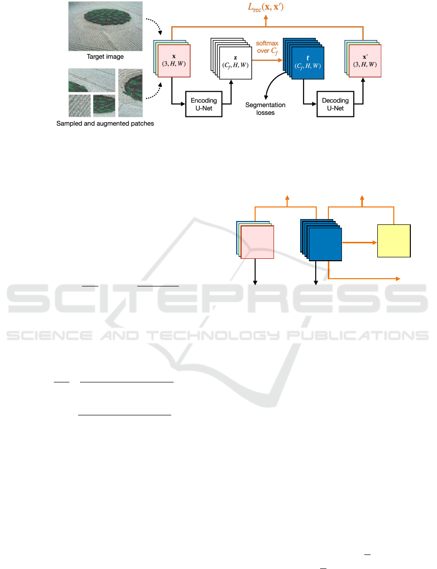
Figure 1: W-Net for dense representation learning with patch reconstruction. The full architecture of the encoding and the

decoding U-Nets can be found in (Xia and Kulis, 2017). The segmentation losses will be computed using the dense features

f, the soft labels for dense segmentation. The size-varying patches are sampled from the input image and then augmented

(ﬂipped or rotated) for training.

The similarity and the continuity loss functions,

originally proposed by (Kim et al., 2020) and often

used together, promote segmentation by clustering f

from two complementary aspects: feature similarity

and spatial continuity. The similarity loss encourages

pixels with similar features to have same the label,

formulated as the cross entropy between f and the ﬁ-

nal label y:

sim

(f, y) = −

∑

log

exp f

i j

∑

exp f

pi j

, (3)

where y can be determined by the channel-wise

argmax of f, i.e., y

i j

= argmax

pi j

. The continuity

loss encourages spatially adjacent pixels to have iden-

tical features (measured in L1), making the segmen-

tation result less patchy:

con

∑

H−1

i=1

∑

| f

pi j

− f

p(i+1) j

(H − 1)W

∑

W −1

j=1

| f

pi j

− f

pi( j+1)

H(W − 1)

(4)

Note that both the similarity and the continuity losses

will ﬁnally lead to a uniform segmentation, i.e., all

pixels having the same label. In (Kim et al., 2020),

the training terminates when the number of differ-

ent labels reaches a lower bound; our model does not

need this lower bound because the reconstruction loss

works as a counterbalance.

2.3 Loss Functions for Sparse

Segmentation

Using superpixels is a divide-and-conquer paradigm

in image and video segmentation. It can signiﬁcantly

reduce the dimensionality and improve the convexity

of the problem, making the model more accurate and

Encoding!

U-Net

Decoding!

U-Net

cut

(f,x)

L1 of adjacent pixels

argmax!

over

(H,W)

sim

(f,y)

con

(f)

…

,H,W)

(3,H,W)

Figure 2: Loss functions for dense segmentation. This ﬁg-

ure and Fig. 1 form the complete architecture for dense seg-

mentation.

easier to train. In this subsection, we extend the above

three segmentation losses to superpixel-based sparse

segmentation. The architecture is shown in Fig. 3.

The ﬁrst step is to determine a RAG based on the

target image, which can be done using a fast super-

pixel method such as SLIC (Achanta et al., 2012)

and the compact watershed (Neubert and Protzel,

2014). Producing a RAG of over-segmentation can

be viewed as a type of weak supervision, as any local

under-segmentation must be avoided manually. How-

ever, as long as a large number of superpixels are al-

lowed by our deep learning model, typically a few

hundreds to a few thousands, our method can remain

fully unsupervised. Suppose the RAG has N

super-

pixels, and the I-th superpixel contains n

pixels. Let

the RAG be represented by a set of dense labels de-

noted by s, that is, the I-th superpixel contains pixel

(i, j) if s

i j

= I. The target image x

pi j

can then be re-

duced to ˆx

by mean colour, ˆx

∑

{(i, j)|s

i j

=I}

pi j

and the features,

∑

{(i, j)|s

i j

=I}

pi j

Based on the reduced image and features, the

sparse extension of the soft N-Cut loss and the sim-

VISAPP 2024 - 19th International Conference on Computer Vision Theory and Applications

578

ilarity loss is straightforward, mostly by replacing

pixel indices to superpixel indices. The sparse soft

N-Cut loss is given by

cut

(

x) = 1 −

∑

p=1

∑

ˆw(I; J)

∑

ˆw(I; J)

, (5)

where ˆw(I;J) measures some distance between super-

pixel I and J, e.g., ˆw(I; J) =

∑

( ˆx

− ˆx

)

. Simi-

larly, the sparse similarity loss is given by

sim

(

y) = −

∑

log

exp f

ˆy

∑

exp

, (6)

where ˆy

is the ﬁnal label of superpixel I, which can

be determined by ˆy

= argmax

. Alternatively, ˆy

can be determined by the maximum occurrence of y

i j

among its encompassed pixels (Kanezaki, 2018), or

by K-means clustering of

along the superpixel di-

mension (to use K-means, change f

ˆy

in eq. (6) into

the centroid of the cluster that I belongs to).

The sparse continuity loss is aimed at uniforming

the features of adjacent superpixels, which is a major

innovation of this work. Let

be the row-wise nor-

malised adjacency matrix of the RAG, that is,

≥ 0,

and

= 0 if superpixel I and J are non-adjacent (in-

cluding I = J), and

∑

= 1. Under this deﬁnition,

∑

yields a weighted average of the p-th fea-

ture over all the neighbours of superpixel I. There-

fore, the continuity loss for sparse segmentation can

be written as

con

∑



∑

−



. (7)

The colour-based weights ˆw(I;J) can be used to deter-

mine

. We will use the following softmax formula

in our experiments:

−τ ˆw(I;J)

∑

−τ ˆw(I;K)

, (8)

where J and K are limited to the neighbours of I.

When the temperature τ = 0, the neighbours of I will

equally contribute to the weighted average

∑

;

otherwise, their contributions will depend on their

distance to I in the colour space. As the total number

of superpixels (N

) increases,

will become larger

and sparser, which can be stored as a sparse tensor.

2.4 Total Loss Function

The total loss is a weighted sum of the reconstruction

loss and the segmentation losses (replacing L with

for sparse segmentation):

L = β

rec

+ β

cut

+ β

sim

+ β

con

, (9)

where the β’s are hyperparameters. Only for dense

segmentation, the above model degenerates to (Xia

and Kulis, 2017) when β

sim

= β

con

= 0 and patch

reconstruction is ignored, and to (Kim et al., 2020)

when β

rec

= β

cut

= 0. Note that our method is not

a simple combination of (Xia and Kulis, 2017) and

(Kim et al., 2020); we borrow their key concepts and

notably improve the accuracy and robustness of the

unsupervised, few-shot model with our augmented

patch reconstruction and sparse loss functions.

We suggest the following steps to fast tune the β-

values, ﬁxing β

rec

= 1 and starting from β

sim

= β

con

(i) Try β

cut

= {0.1, 1, 10} and select the best; avoid

under-segmentation at this step;

(ii) Fixing β

cut

, try β

sim

= β

con

= {0.1, 1, 10} and

select the best; increase β

con

if the result looks

too patchy, and decrease β

con

if the result suffers

under-segmentation; and

(iii) do ﬁne-tuning if necessary.

3 EXPERIMENTS

3.1 Single-Image Benchmark

In this experiment, we evaluate our method using the

100 test images from BSDS300 (Martin et al., 2001).

For each image, we train models of nine types using

the same W-Net architecture but with different seg-

mentation and reconstruction losses. For the segmen-

tation losses, we consider pixel or superpixel ones

(Dense vs Sparse), and N-Cut alone or combining

similarity and continuity (NCut vs SimCon). Here, we

separate N-Cut from similarity and continuity to re-

duce the number of hyperparameters (β’s in eq. (9)).

For reconstruction loss, we consider a single image or

sampled patches (Image vs Patch). Such variability

leads to eight different model types in total:

1. Dense-NCut-Image,

2. Dense-NCut-Patch,

3. Dense-SimCon-Image,

4. Dense-SimCon-Patch,

5. Sparse-NCut-Image,

6. Sparse-NCut-Patch,

7. Sparse-SimCon-Image and

8. Sparse-SimCon-Patch.

The type Dense-NCut-Image is equivalent to the

original W-Net (Xia and Kulis, 2017). We train

an additional type of models, Dense-SimCon-NoRec,

Unsupervised Few-Shot Image Segmentation with Dense Feature Learning and Sparse Clustering

579

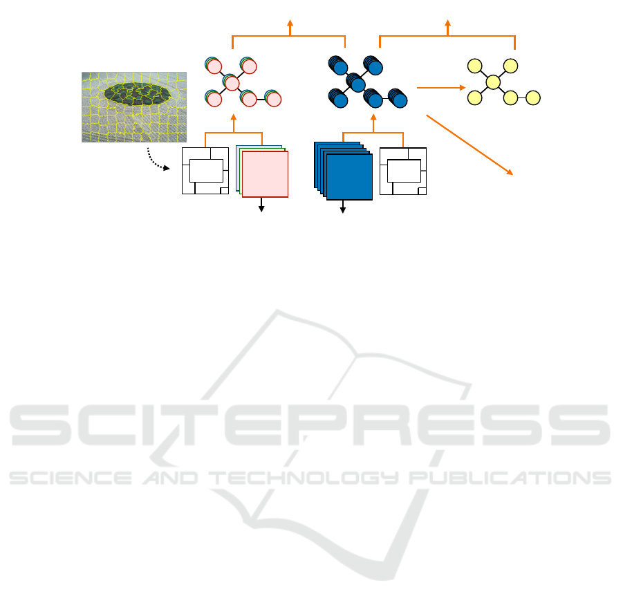
Encoding!

U-Net

Decoding!

U-Net

Reduce

argmax!

over

Reduce

L1 of adjacent nodes

cut

(

sim

(

con

(

…

(H,W)

(3,H,W)

,H,W)

(H,W)

)

(3,N

)

RAG

Figure 3: Loss functions for sparse segmentation. This ﬁgure and Fig. 1 form the complete architecture for sparse segmen-

tation. The RAG of the target image, as represented by its dense labels, s = {s

i j

}, is predetermined using a fast superpixel

method such as SLIC, which contains N

segments in total.

where NoRec means no reconstruction (i.e., decoder

unused), which corresponds to the original dense

model of (Kim et al., 2020). For each of these model

types, we consider ten random states for model initial-

isation and nine β-values for the segmentation losses

β = {5, 2, 1, 0.5, 0.2, 0.1, 0.05, 0.02, 0.01} while ﬁx-

ing β

rec

= 1. The superpixels are prepared using SLIC

with from 3, 000 to 8, 000 segments. For each im-

age, we sample 232 patches in total: 32 × (96, 96) +

72×(64, 64)+128×(48, 48), each shape divided into

eight mini-batches. We use the Adam optimiser with

a learning rate of 10

−3

and train the models for 50

epochs.

To evaluate the outcomes of segmentation, we cal-

culate six clustering metrics: random index, adjusted

mutual information, the Fowlkes-Mallows index, ho-

mogeneity, completeness and V-measure. Here, we

emphasise the signiﬁcance of homogeneity and com-

pleteness (V-measure being their harmonic mean)

from the angle of post-processing, aimed at reﬁn-

ing the outcome of unsupervised segmentation, e.g.,

(Xia and Kulis, 2017). Homogeneity measures

how the resultant segmentation is close to a per-

fect over-segmentation, and completeness how that

is close to a perfect under-segmentation. For ex-

ample, our sparse model starts from homogeneity≈1

and completeness≈0 at the beginning of training. At

post-processing, it is much easier to merge a few seg-

ments from an over-segmentation than to separate dif-

ferent segments from an under-segmentation. There-

fore, a low completeness may be remedied by post-

processing while a low homogeneity tends to veto.

An unsupervised method should try to avoid low ho-

mogeneity while increasing completeness as much as

possible. Note that supervised metrics such as IoU

and F1 cannot be used without manually associating

the predicted and true labels.

The metric scores of the different models are

shown in Table 1, which can be summarised as fol-

lows. First, from a reconstruction perspective, us-

ing sampled patches (Patch) has led to higher scores

than using a single image (Image) and no reconstruc-

tion (NoRec). Second, sparse labelling (Sparse) has

achieved higher scores than dense labelling (Dense),

regardless of reconstruction or segmentation losses.

Finally, comparing N-Cut alone (NCut) to the combi-

nation of similarity and continuity (SimCon), the latter

has obtained higher scores for all the considered met-

rics except for homogeneity (where the difference is

small), indicating that N-Cut is more inclined toward

over-segmentation. In practice, these three segmenta-

tion losses can be used together for best performance.

3.2 Videos

The capability for 3D prediction is a critical property

of an unsupervised model trained with one or a few

2D images. One reason is that an unsupervised model

usually demands more efforts for hyperparameter tun-

ing and random state sampling, and such a capability

can make the best of these efforts. Here, we show

two video examples in Fig. 4. In (a), a jump from

a ﬁgure skater, we only use the ﬁrst frame for train-

ing, and the resultant sparse model can well predict

the remaining frames containing the trajectory of the

motions of the skater. The dense models we trained

failed to ﬁnd the boundary near the skater’s shoulders

(where his costume is ice-coloured). In (b), a cheetah

hunting a gazelle, we train a sparse model with three

frames: the ﬁrst and the third are focused respectively

VISAPP 2024 - 19th International Conference on Computer Vision Theory and Applications

580

Table 1: Metric scores of different models for test images in BSDS300. The name of the dense and the sparse models are

explained in the text. The three baseline models are K-means on pixels, K-Means on superpixels, and spectral clustering

on superpixels. The six metrics are random index (RI), adjusted mutual information (A-MI), Fowlkes-Mallows index (FMI),

homogeneity (Homo), completeness (Comp), and V-measure (V-M). For each image and model type, we select the ﬁnal model

(from ten random states × nine β-values) by the highest V-measure, based on which the other metrics are computed. The

results of some of the images are displayed in the Appendix.

Model type RI A-MI FMI Homo Comp V-M

Dense models Dense-NCut-Image 0.77 0.45 0.62 0.43 0.50 0.45

Dense-NCut-Patch 0.77 0.51 0.62 0.58 0.49 0.51

Dense-SimCon-Image 0.77 0.47 0.65 0.43 0.56 0.47

Dense-SimCon-Patch 0.80 0.55 0.70 0.52 0.63 0.55

Dense-SimCon-NoRec 0.78 0.52 0.67 0.49 0.59 0.52

Sparse models Sparse-NCut-Image 0.77 0.46 0.63 0.45 0.51 0.46

Sparse-NCut-Patch 0.79 0.55 0.64 0.63 0.52 0.55

Sparse-SimCon-Image 0.79 0.52 0.69 0.46 0.63 0.52

Sparse-SimCon-Patch 0.81 0.57 0.71 0.60 0.66 0.63

Baseline models Kmeans-Pixel 0.69 0.31 0.49 0.31 0.34 0.31

Kmeans-Superpixel 0.71 0.33 0.50 0.33 0.37 0.33

Spectral-Superpixel 0.72 0.39 0.55 0.39 0.43 0.39

on the cheetah and the gazelle, and in the second one,

the cheetah’s body is partially covered by a wisp of

grass. Dense segmentation could also outline the two

animals correctly but delivered an inferior accuracy

for depicting their boundaries in detail.

4 APPLICATION: X-RAY AND

NEUTRON IMAGING

Large-scale experimental facilities, such as linear ac-

celerators and synchrotrons using X-ray or neutron

sources, offer a powerful means for probing the in-

ternal structure of condensed matters from nano- to

micro-scales (Sivia, 2011). In this section, we train

models to segment 3D tomographic images obtained

from X-ray and neutron imaging.

Compared to real-world photographic images,

tomographic images are usually less semantically

meaningful, characterised by less deﬁnitive bound-

aries between parts and lower signal-to-noise ratios.

Unless the scanned sample has a very simple struc-

ture with strong contrasts, ﬁnding the ground truth of

segmentation is mostly impossible. However, in the

context of unsupervised segmentation, these 3D im-

ages can beneﬁt from a high similarity between their

2D slices, allowing us to train a 2D model with one

or a few slices. In all the three experiments presented

here, we will use only one 2D slice for training.

Figure 5 shows the target tomographic images and

their segmentation results. In (a), the foreground is

a thin crack in an Alloy 2205 duplex stainless steel,

scanned by X-ray tomography. The original images

are characterised by high-frequency, diffusive fea-

tures, which pose a great challenge to segmentation.

Therefore, we blur the slices with a Gaussian ﬁlter

and use its Hessian for segmentation, following (Kang

et al., 2020). In the second and the third examples, the

same rock core sample is scanned respectively by X-

rays and neutrons, but the tomographic images look

distinct. X-rays deliver a high-deﬁnition structure

containing micro-cracks and bright spots (possibly re-

gions containing high-Z elements). Neutrons, on the

other hand, yield a ﬂocculent structure with lower res-

olution, highlighting regions of hydrogen-containing

minerals (red). We do not attempt to fuse the X-ray

and neutron data but treat them as two independent

problems. For all the three datasets, our segmentation

results turn out satisfactory by visual inspection, with

all structural features correctly detected and labelled.

Without the ground truths, however, we cannot per-

form quantitative evaluation on these results.

5 CONCLUSIONS

We have developed a new and easy-to-use deep learn-

ing method for fully unsupervised semantic segmen-

tation of images, which has achieved satisfactory ac-

curacy across a set of 2D images, videos and 3D

tomographic images. We use a W-Net architecture

for dense or pixel-based feature learning; the learned

dense features are reduced onto a regional adjacency

graph (RAG) whereby segmentation is achieved by

three sparse or superpixel-based loss functions, re-

spectively accounting for normalised cut, similarity

and continuity. Our sparse continuity loss allows

a large number of superpixels in the RAG so that

preparing the RAG can remain fully unsupervised.

Unsupervised Few-Shot Image Segmentation with Dense Feature Learning and Sparse Clustering

581

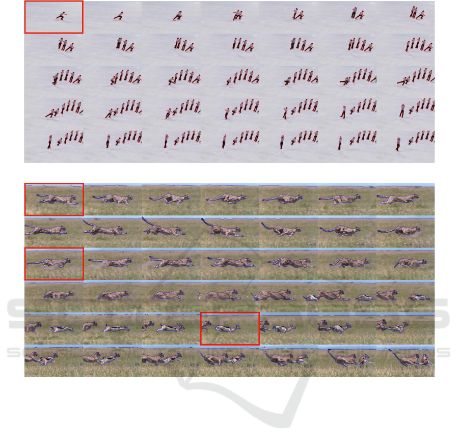
(a) A jump from a ﬁgure skater (80 frames).

(b) A cheetah hunting a gazelle (402 frames).

Figure 4: Unsupervised segmentation of videos. Only the boxed frames are used for training. For both (a) and (b), we use

Sparse-SimCon-Patch with β

sim

= β

con

= 0.1. For (a), patch sampling is limited to a small vicinity of the foreground.

Also, regularising segmentation with our augmented

patch reconstruction can greatly mitigate overﬁtting

caused by few-shot learning. This work has followed

the key concepts of (Xia and Kulis, 2017) and (Kim

et al., 2020), while having notably improved the per-

formance of the unsupervised, few-shot model with

the above novel techniques.

Our quantitative experiment on the BSDS300

dataset shows that using our patch sampling for re-

construction and performing segmentation on super-

pixels have led to more accurate and robust results.

We have also carried out qualitative experiments us-

ing videos and 3D images acquired from X-ray and

neutron tomography. These 3D experiments show

that our model trained with one or a few images (no

labels) can be highly robust for predicting unseen

images with similar semantic contents. Therefore,

our method can be powerful for the segmentation of

videos and 3D images of this kind with one- or few-

shot learning in 2D.

ACKNOWLEDGEMENTS

This work is funded by the Ada Lovelace Centre,

Rutherford Appleton Laboratory, Science and Tech-

nology Facilities Council. The computing resources

are funded by the IRIS initiative. The X-ray and neu-

tron data are obtained from the Diamond Light Source

and the ISIS Neutron and Muon Source, respectively.

VISAPP 2024 - 19th International Conference on Computer Vision Theory and Applications

582

(a) A crack from X-ray imaging (30 slices).

(b) A rock from X-ray imaging (801 slices).

Figure 5: Unsupervised segmentation of 3D images from X-ray and neutron tomography. The original images are shown

on the left, the 2D labels in the middle and the 3D labels on the right. Only one slice (boxed) is used for training in each

case. We use Sparse-NCut-Patch with β

cut

= 1 for (a), Sparse-SimCon-Patch with β

sim

= β

con

= 0.002 for (b), and

Sparse-SimCon-Patch with β

sim

= β

con

= 0.1 for (c). Segmentation of (a) is based on the Hessian of the original images

smoothened by a Gaussian ﬁlter.

Unsupervised Few-Shot Image Segmentation with Dense Feature Learning and Sparse Clustering

583

REFERENCES

Achanta, R., Shaji, A., Smith, K., Lucchi, A., Fua, P., and

usstrunk, S. (2012). Slic superpixels compared to

state-of-the-art superpixel methods. IEEE transac-

tions on pattern analysis and machine intelligence,

34(11):2274–2282.

Aksoy, Y., Oh, T.-H., Paris, S., Pollefeys, M., and Matusik,

W. (2018). Semantic soft segmentation. ACM Trans-

actions on Graphics (TOG), 37(4):1–13.

Badrinarayanan, V., Kendall, A., and Cipolla, R. (2017).

Segnet: A deep convolutional encoder-decoder ar-

chitecture for image segmentation. IEEE transac-

tions on pattern analysis and machine intelligence,

39(12):2481–2495.

Bianchi, F. M., Grattarola, D., and Alippi, C. (2020). Spec-

tral clustering with graph neural networks for graph

pooling. In International Conference on Machine

Learning, pages 874–883. PMLR.

Brown, E. S., Chan, T. F., and Bresson, X. (2012). Com-

pletely convex formulation of the chan-vese image

segmentation model. International journal of com-

puter vision, 98(1):103–121.

Chen, L.-C., Papandreou, G., Kokkinos, I., Murphy, K., and

Yuille, A. L. (2017). Deeplab: Semantic image seg-

mentation with deep convolutional nets, atrous convo-

lution, and fully connected crfs. IEEE transactions on

pattern analysis and machine intelligence, 40(4):834–

848.

Chen, Q., Huang, Y., Sun, H., and Huang, W. (2021). Pave-

ment crack detection using hessian structure propaga-

tion. Advanced Engineering Informatics, 49:101303.

Criminisi, A., Sharp, T., Rother, C., and P

erez, P. (2010).

Geodesic image and video editing. ACM Trans.

Graph., 29(5):134–1.

Danon, D., Averbuch-Elor, H., Fried, O., and Cohen-Or, D.

(2019). Unsupervised natural image patch learning.

Computational Visual Media, 5(3):229–237.

Eliasof, M., Zikri, N. B., and Treister, E. (2022). Un-

supervised image semantic segmentation through su-

perpixels and graph neural networks. arXiv preprint

arXiv:2210.11810.

Hofmarcher, M., Unterthiner, T., Arjona-Medina, J., Klam-

bauer, G., Hochreiter, S., and Nessler, B. (2019). Vi-

sual scene understanding for autonomous driving us-

ing semantic segmentation. In Explainable AI: Inter-

preting, Explaining and Visualizing Deep Learning,

pages 285–296. Springer.

Hsu, J., Gu, J., Wu, G., Chiu, W., and Yeung, S.

(2021). Capturing implicit hierarchical structure in

3d biomedical images with self-supervised hyperbolic

representations. Advances in Neural Information Pro-

cessing Systems, 34:5112–5123.

Ibrahim, A. and El-kenawy, E.-S. M. (2020). Image seg-

mentation methods based on superpixel techniques: A

survey. Journal of Computer Science and Information

Systems, 15(3):1–11.

Ji, X., Henriques, J. F., and Vedaldi, A. (2019). Invariant

information clustering for unsupervised image clas-

siﬁcation and segmentation. In Proceedings of the

IEEE/CVF International Conference on Computer Vi-

sion, pages 9865–9874.

Kanezaki, A. (2018). Unsupervised image segmentation by

backpropagation. In 2018 IEEE international con-

ference on acoustics, speech and signal processing

(ICASSP), pages 1543–1547. IEEE.

Kang, D., Benipal, S. S., Gopal, D. L., and Cha, Y.-J.

(2020). Hybrid pixel-level concrete crack segmenta-

tion and quantiﬁcation across complex backgrounds

using deep learning. Automation in Construction,

118:103291.

Kim, W., Kanezaki, A., and Tanaka, M. (2020). Unsuper-

vised learning of image segmentation based on dif-

ferentiable feature clustering. IEEE Transactions on

Image Processing, 29:8055–8068.

Lambert, Z., Le Guyader, C., and Petitjean, C. (2021). A

geometrically-constrained deep network for ct image

segmentation. In 2021 IEEE 18th International Sym-

posium on Biomedical Imaging (ISBI), pages 29–33.

IEEE.

Lempitsky, V., Kohli, P., Rother, C., and Sharp, T. (2009).

Image segmentation with a bounding box prior. In

2009 IEEE 12th international conference on computer

vision, pages 277–284. IEEE.

Lin, D., Dai, J., Jia, J., He, K., and Sun, J. (2016). Scribble-

sup: Scribble-supervised convolutional networks for

semantic segmentation. In Proceedings of the IEEE

conference on computer vision and pattern recogni-

tion, pages 3159–3167.

Lin, G., Milan, A., Shen, C., and Reid, I. (2017). Reﬁnenet:

Multi-path reﬁnement networks for high-resolution

semantic segmentation. In Proceedings of the IEEE

conference on computer vision and pattern recogni-

tion, pages 1925–1934.

Martin, D., Fowlkes, C., Tal, D., and Malik, J. (2001).

A database of human segmented natural images and

its application to evaluating segmentation algorithms

and measuring ecological statistics. In Proc. 8th Int’l

Conf. Computer Vision, volume 2, pages 416–423.

Minaee, S., Boykov, Y. Y., Porikli, F., Plaza, A. J., Kehtar-

navaz, N., and Terzopoulos, D. (2021). Image seg-

mentation using deep learning: A survey. IEEE trans-

actions on pattern analysis and machine intelligence.

Mirsadeghi, S. E., Royat, A., and Rezatoﬁghi, H. (2021).

Unsupervised image segmentation by mutual infor-

mation maximization and adversarial regularization.

IEEE Robotics and Automation Letters, 6(4):6931–

6938.

Moriya, T., Roth, H. R., Nakamura, S., Oda, H., Nagara,

K., Oda, M., and Mori, K. (2018). Unsupervised seg-

mentation of 3d medical images based on clustering

and deep representation learning. In Medical Imaging

2018: Biomedical Applications in Molecular, Struc-

tural, and Functional Imaging, volume 10578, pages

483–489. SPIE.

Neubert, P. and Protzel, P. (2014). Compact watershed

and preemptive slic: On improving trade-offs of su-

perpixel segmentation algorithms. In 2014 22nd in-

ternational conference on pattern recognition, pages

996–1001. IEEE.

VISAPP 2024 - 19th International Conference on Computer Vision Theory and Applications

584

Ouali, Y., Hudelot, C., and Tami, M. (2020). Autoregressive

unsupervised image segmentation. In European Con-

ference on Computer Vision, pages 142–158. Springer.

Ronneberger, O., Fischer, P., and Brox, T. (2015). U-net:

Convolutional networks for biomedical image seg-

mentation. In International Conference on Medical

image computing and computer-assisted intervention,

pages 234–241. Springer.

Scatigno, C. and Festa, G. (2022). Neutron imaging and

learning algorithms: New perspectives in cultural her-

itage applications. Journal of Imaging, 8(10):284.

Sivia, D. S. (2011). Elementary scattering theory: for X-ray

and neutron users. Oxford University Press.

Verdoja, F., Thomas, D., and Sugimoto, A. (2017). Fast

3d point cloud segmentation using supervoxels with

geometry and color for 3d scene understanding. In

2017 IEEE International Conference on Multimedia

and Expo (ICME), pages 1285–1290. IEEE.

Xia, X. and Kulis, B. (2017). W-net: A deep model for fully

unsupervised image segmentation. arXiv preprint

arXiv:1711.08506.

Xiao, C. and Bufﬁere, J.-Y. (2021). Neural network seg-

mentation methods for fatigue crack images obtained

with x-ray tomography. Engineering Fracture Me-

chanics, 252:107823.

Yang, W., Luo, P., and Lin, L. (2014). Clothing co-parsing

by joint image segmentation and labeling. In Proceed-

ings of the IEEE conference on computer vision and

pattern recognition, pages 3182–3189.

Yin, S., Qian, Y., and Gong, M. (2017). Unsupervised hi-

erarchical image segmentation through fuzzy entropy

maximization. Pattern Recognition, 68:245–259.

Yu, H., He, F., and Pan, Y. (2020). A survey of level

set method for image segmentation with intensity in-

homogeneity. Multimedia Tools and Applications,

79(39):28525–28549.

Yu, J., Huang, D., and Wei, Z. (2018). Unsupervised im-

age segmentation via stacked denoising auto-encoder

and hierarchical patch indexing. Signal Processing,

143:346–353.

Zhang, J., Yang, P., Wang, W., Hong, Y., and Zhang, L.

(2020). Image editing via segmentation guided self-

attention network. IEEE Signal Processing Letters,

27:1605–1609.

Zhao, H., Qi, X., Shen, X., Shi, J., and Jia, J. (2018).

Icnet for real-time semantic segmentation on high-

resolution images. In Proceedings of the European

conference on computer vision (ECCV), pages 405–

420.

Zhao, H., Shi, J., Qi, X., Wang, X., and Jia, J. (2017).

Pyramid scene parsing network. In Proceedings of

the IEEE conference on computer vision and pattern

recognition, pages 2881–2890.

Zhou, L. and Wei, W. (2020). Dic: deep image clustering

for unsupervised image segmentation. IEEE Access,

8:34481–34491.

Unsupervised Few-Shot Image Segmentation with Dense Feature Learning and Sparse Clustering

585

APPENDIX

Figure 6 shows the segmentation results for some of

the test images from BSDS300.

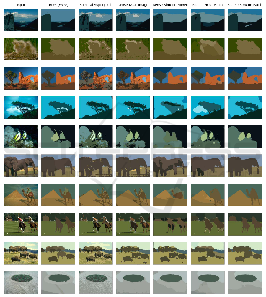
Figure 6: Segmentation results for some test images in BSDS300. The ﬁrst and second columns show the input images and

their ground truths. The third column contains the results from Spectral-Superpixel, a baseline solution using spectral

clustering on the superpixels. The fourth and the ﬁfth columns show the results from two of our dense models, respectively

corresponding to the models of (Xia and Kulis, 2017) and (Kim et al., 2020). The last two columns show the results from two

of our sparse models using different segmentation losses.

VISAPP 2024 - 19th International Conference on Computer Vision Theory and Applications

586