Scale Learning in Scale-Equivariant Convolutional Networks

Mark Basting

, Robert-Jan Bruintjes

, Thadd

aus Wiedemer

2,3

, Matthias K

ummerer

Matthias Bethge

2,4

and Jan van Gemert

Computer Vision Lab, Delft University of Technology, The Netherlands

Bethgelab, University of T

ubingen, Geschwister-Scholl-Platz, T

ubingen, Germany

Machine Learning, Max-Planck-Institute for Intelligent Systems, Max-Planck-Ring, T

ubingen, Germany

ubingen AI Center, Maria-von-Linden-Straße, T

ubingen, Germany

Keywords:

Convolutional Neural Networks, Scale, Scale-Equivariance, Scale Learning.

Abstract:

Objects can take up an arbitrary number of pixels in an image: Objects come in different sizes, and, pho-

tographs of these objects may be taken at various distances to the camera. These pixel size variations are

problematic for CNNs, causing them to learn separate ﬁlters for scaled variants of the same objects which pre-

vents learning across scales. This is addressed by scale-equivariant approaches that share features across a set

of pre-determined ﬁxed internal scales. These works, however, give little information about how to best choose

the internal scales when the underlying distribution of sizes, or scale distribution, in the dataset, is unknown.

In this work we investigate learning the internal scales distribution in scale-equivariant CNNs, allowing them

to adapt to unknown data scale distributions. We show that our method can learn the internal scales on various

data scale distributions and can adapt the internal scales in current scale-equivariant approaches.

1 INTRODUCTION

Objects in images naturally occur at various scales.

The scale, or size in terms of pixels, of an object in an

image can vary because of perspective effects stem-

ming from the distance to the camera or due to in-

terclass variation. For example, imagine a golf ball

and a volleyball being classiﬁed as balls but varying in

size. Vanilla CNNs can learn differently-sized objects

when presented with large amounts of data. However,

since the CNN has no internal notion of scale, sepa-

rate ﬁlters for differently scaled versions of the same

objects are learned, leading to signiﬁcant redundancy

in the learned features.

Scale-equivariant CNNs such as (Xu et al., 2014a;

Sosnovik et al., 2019) share features across a ﬁxed

set of chosen internal scales which increases parame-

ter efﬁciency by removing the need to learn separate

ﬁlters for differently-sized objects. Yet, such scale-

convolution approaches need tune the internal scales

as a hyper-parameter. Instead, here, We present a

model that can learn these internal scales.

In this paper, we present a model of the relation-

ship between the internal scales and the data scale

distribution. We show empirically the parameters for

which this model is most accurate. Furthermore, we

deﬁne a parameterization of the internal scales and

draw inspiration from NJet-Net (Pintea et al., 2021)

to learn the internal scales. Our method provides a

way to learn the internal scales without the need for

prior knowledge of the scale distribution of your data.

We have the following contributions. 1. We

demonstrate that the best internal scales are related

to the used data scale distribution. 2. We derive an

empirical model that shows approximately how we

should choose the internal scales when the data scale

distribution is known. 3. We remove the need for

prior knowledge about the data scale distribution by

making the internal scales learnable.

2 RELATED WORK

Scale Spaces. Scale is naturally deﬁned on a loga-

rithmic axis (Florack et al., 1992; Lindeberg and Ek-

lundh, 1992) We base our work on Gaussian scale-

space theory and use theory on the logarithmic nature

of scale to deﬁne the internal scale tolerance model

and in the parameterisation of the internal scales.

Pyramid Networks. These use differently scaled

versions of the input image to share features across

different scales. Popular pyramid networks in-

clude (Farabet et al., 2013; Kanazawa et al., 2014;

Marcos et al., 2018), and are equivariant over ﬁxed

Basting, M., Bruintjes, R., Wiedemer, T., Kümmerer, M., Bethge, M. and van Gemert, J.

Scale Learning in Scale-Equivariant Convolutional Networks.

DOI: 10.5220/0012379800003660

Paper published under CC license (CC BY-NC-ND 4.0)

In Proceedings of the 19th International Joint Conference on Computer Vision, Imaging and Computer Graphics Theory and Applications (VISIGRAPP 2024) - Volume 2: VISAPP, pages

567-574

ISBN: 978-989-758-679-8; ISSN: 2184-4321

567

chosen scales and require many expensive interpola-

tion operations. Contrarily, our approach can learn

the scales without extensive use of interpolations.

Scale Group Convolutions. An alternative way

to achieve scale-equivariance or scale-invariance is

through the use of group convolution (Xu et al.,

2014a; Sosnovik et al., 2019; Ghosh and Gupta, 2019;

Naderi et al., 2020; Zhu et al., 2019; Lindeberg,

2020). DISCO (Sosnovik et al., 2021) argues that

the discretisation of the underlying continuous basis

functions leads to increased scale-equivariance error

and therefore leads to worse performance. Instead,

they opt to use dilation for integer scale factors and di-

rectly optimise basis functions for non-integer scales

using the scale-equivariance error (Sosnovik et al.,

2021). While all methods allow for non-integer scale

factors, the scales over which the network is equiv-

ariant are ﬁxed and they provide little instructions on

how to best choose the internal scales.

Learnable Scale. Continuous kernel parameterisa-

tion forms the basis of methods that aim to learn the

scale or scales of the dataset (Pintea et al., 2021; Sal-

danha et al., 2021; Tomen et al., 2021; Yang et al.,

2023; Benton et al., 2020; Sun and Blu, 2023). The

NJet-Net (Pintea et al., 2021) learned the scale of the

dataset by making the σ parameter of the Gaussian

derivative basis function learnable. We build on that

work to learn multiple internal scales simultaneously.

3 METHOD

In Fig. 1 we visualize the setting. Our method is

equivariant to both translation and scale transforma-

tions. Like SESN (Sosnovik et al., 2019), our method

achieves scale-equivariance through an inverse map-

ping of the kernel:

[ f ] ∗κ = L

[ f ∗ κ

−1

], ∀ f , s (1)

where L

represents a scaling transformation by a fac-

tor s, κ is a discretized continuous kernel parameter-

ized by an inner scale. Thus, a scaled input convolved

with a kernel is the same as ﬁrst convolving the origi-

nal input with an inversely scaled kernel and then ap-

plying the same scaling.

Due to the discrete nature of images, we need to

approximate the equivariance to translation and scal-

ing by a discrete group. The translation group is ap-

proximated by taking into account all discrete trans-

lations. The scaling group is discretised by N

scales

with log-uniform spacing as follows:

S = [σ

basis

× ISR

(

−1

)

for i in 0..N

− 1] (2)

𝐼𝑆𝑅

𝜎

𝑏𝑎𝑠𝑖𝑠

𝑆

Internal Scales

Trainable Scale

Parameters

Dynamic Filter Basis

× =

𝑤

Generate

Trainable

Weights

𝑤

Multi-Scale

Kernel

Figure 1: Dynamic Multi-Scale Kernel generation pipeline.

Filter basis is parameterised by a discrete set of scales which

in turn are generated from learnable parameters, controlling

both the size of the ﬁrst scale σ

basis

and the range the inter-

nal scales span (ISR). Linear combination of the Dynamic

Filter Basis functions with trainable weights form Multi-

Scale Kernel.

where σ

basis

is a learnable parameter that deﬁnes the

smallest scale, and the ISR deﬁnes the range between

the largest and smallest scale, also known as the In-

ternal Scale Range. The logarithmic spacing can be

attributed to the logarithmic nature of the scale.

The kernels of the model consist of a weighted

sum of basis functions that are deﬁned at each scale

in the internal scales S . Following (Sosnovik et al.,

2019), we use a basis of 2D Hermite polynomials with

a 2D Gaussian envelope. This basis is pre-computed

at the start of training for all pre-determined scales if

scale learning is disabled. Otherwise, the basis func-

tions are recomputed at each forward pass.

Scale-Convolution. Scale-convolution is a standard

convolution extended by incorporating an additional

scale dimension (Sosnovik et al., 2019). Without tak-

ing into account interscale interactions we deﬁne the

following two types of scale convolutions:

1. Conv T → H: In this scenario, the input of the

scale-convolution is a tensor without any scale-

dimension, or |S

′

| = 1. The output, deﬁned over

the internal scales S stems from the convolution of

the input with scaled kernels κ

−1

s.t. s ∈ S:

[ f ∗

κ](s, t) = f (·) ∗ κ

−1

(·) (3)

where κ

is a kernel scaled by s, ∗

is the scale

convolution and ∗ is a standard convolution.

2. Conv H → H: The input is now deﬁned over the

internal scales S, the resulting output at scale s

is the convolution of the input at scale s with the

scaled kernel κ

−1

[ f ∗

κ](s, t) = f (s, ·) ∗ κ

−1

(·) (4)

These methods are designed to adhere to the scale-

equivariance equation highlighted in Eq. 1.

VISAPP 2024 - 19th International Conference on Computer Vision Theory and Applications

568

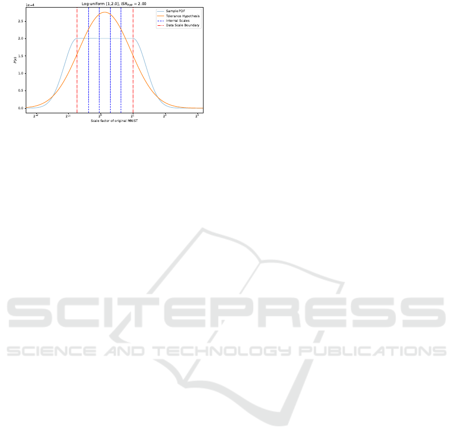
Figure 2: Example of possible internal scale tolerance

model for the log-uniform data scale distribution over the

range [0.6, 2.0] with ISR

hyp

ﬁxed to 2 to reﬂect internal

scales choice in SESN (Sosnovik et al., 2019) on MNIST-

Scale.

Internal Scale Tolerance Model. We deﬁne an em-

pirical tolerance model to estimate which internal

scales to choose when the scale distribution is known.

The tolerance describes the region of data scales the

kernel can generalise to. Previous papers have shown

that the generalisation error to unseen scales follows

an approximate log-normal distribution (Kanazawa

et al., 2014; Lindeberg, 2020). Therefore, we use a

Normal distribution on a logarithmic scale to model

the tolerance for each kernel at a certain internal scale.

The log-normal distributions of each internal scale are

then combined into one mixture model. An example

of a possible conﬁguration can be seen in Fig. 2.

The internal scale tolerance model has the following

parameters:

1. Reference Internal Scale: deﬁnes the relationship

between the position of the internal scales and the

data scales.

2. ISR

hyp

: range over which the internal scales are

deﬁned, this is the factor between the largest and

the smallest scale.

3. τ

tol

: standard deviation of the underlying log-

normal distribution that is placed on each internal

scale.

The reference scale and ISR are speciﬁc to each

tolerance model of a data scale distribution while τ

tol

is independent of the data scale distribution and a

property of a kernel.

We make the assumption here that we do know the

data scale distribution. We extend the data scale dis-

tribution at the boundaries by a half-log-normal dis-

tribution with σ = 0.4 to model the generalisation to

unseen scales. The Kullback-Leibler (Kullback and

Leibler, 1951) is used to ﬁt the tolerance model on

the data scale sampling distributions.

Moving Away from Fixed Scale Groups. To make

the scales of the network learnable we move away

from ﬁxed multi-scale basis functions and make the

scales of the basis functions dynamic. The scales that

parameterise the basis functions are continuous and

have a gradient with regard to the loss allowing for

direct optimisation. This allows us to simultaneously

learn the kernel shape and scales, see Fig. 1. Unlike

SEUNET (Yang et al., 2023), we do not parameterise

the scales directly but parameterise the internal scales

by σ

basis

and the ISR using Eq. 5.

We observe that a value for the ISR lower or equal

to 1 is unwanted as this would result in kernels at the

same scale or a subsequent scale smaller than the base

scale deﬁned by σ

basis

. We do not use a ReLU acti-

vation as this can lead to a dead neuron and zero gra-

dient. We parameterise the ISR using the following

formula:

ISR = 1 + γ

(5)

where γ is the learnable parameter. We will only men-

tion the ISR since it is closely related to the learnable

parameter and more intuitive to understand.

Various size basis functions lead to difﬁculties in

choosing the best kernel size before training. We use

the method by (Pintea et al., 2021) to learn the size of

the kernel based on the ISR:

l = 2⌈k(σ

basis

× ISR)⌉ + 1 (6)

where k is a hyperparameter that determines the ex-

tent of the approximation of the continuous basis

functions. Thus, the kernel size used in convolution

is determined by the largest scale in the set of internal

scales which is directly parameterised by σ

basis

and

the ISR.

4 EXPERIMENTS

In Section 4.1 and 4.2, we use the simple architecture

shown in Tab. 1 on the commonly used MNIST-Scale

dataset (Kanazawa et al., 2014) with a Logarithmi-

cally Uniform data scale distribution with a range of 1

to 2

1.5

, 2

2.25

and 2

corresponding to 2.83, 4.76, and 8

scale factors of MNIST respectively. Appx. 5 gives a

complete description of all datasets used in the exper-

iments.

4.1 Validation

Do Internal Scales Really Matter? We test our as-

sumption that the internal scale range (ISR), the factor

between the largest and smallest internal scale inﬂu-

ences the performance. Furthermore, we compare the

Scale Learning in Scale-Equivariant Convolutional Networks

569

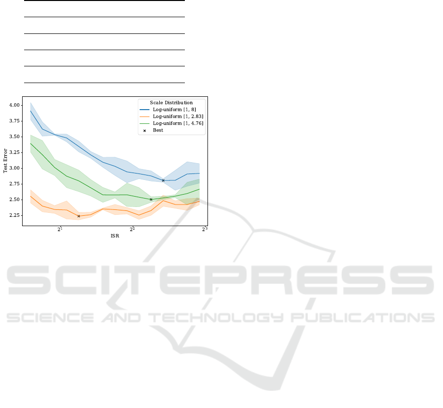
Table 1: CNN for Experiments 4.1 and 4.2 to show the im-

pact of choosing the internal scales and scale-learning.

Conv T → H, Hermite, N

= 3, 16 ﬁlters

scale-projection

batch norm, relu

42 x 42 max pool

fully-connected, softmax

Figure 3: Impact on Test Error when varying Internal Scale

Range (ISR) for different log-uniform data scale distribu-

tions from 1 scale factor of MNIST to 2.83, 4.76 and 8 scale

factors MNIST. The value of the Internal Scale Range (ISR)

for the best-performing model increases together with the

width of the model.

optimal ISRs we discovered with the suggested val-

ues of the Internal Scale Tolerance model. The ISRs

are chosen on a logarithmic scale in the range of [1.5,

7.65].

The results in Fig. 3 indicate that smaller ISRs

are better for narrow data scale distributions, while

larger ISRs perform better for wider data scale dis-

tributions. Thus, for a log-uniform distribution that

spans a small scale range narrow internal scales are

preferred. Conversely, for a log-uniform distribution

that spans a large scale range, wide internal scales

are preferred. Looking at the test error of individ-

ual data scales in Fig. 4, we see that at the bound-

ary regions of wide scale distributions narrow inter-

nal scales achieve signiﬁcantly higher test error than

wider internal scales indicating that the model can-

not share features across the whole data scale distri-

bution. Narrow internal scales perform slightly better

than wider internal scales when evaluated on narrow

distributions. This statement aligns with results found

in Fig. 3, which indicates less test error variation be-

tween ISR values for the log-uniform distribution be-

tween 1 and 2.83.

The results of the combined optimisation of the

tolerant model and the three sampling distributions

can be found in Fig. 5. The optimisation leads to

tol

= 0.459. The optimisation ﬁts ISR values ap-

proximately similar to the best ISRs depicted in Fig.

3. Again, the ISR values follow an increasing pattern

when the data scale distribution gets wider. Addition-

ally, Fig. 5 shows increasing gaps in the tolerance

hypothesis between internal scales for wide distribu-

tions.

Can We Learn the Internal Scales? To test our

scale-learning capabilities, we evaluate our scale-

learning on three log-uniform data scale distributions.

The ISR is parameterised according to Eq. 5 and

the scale parameters are initialised with σ

basis

= 2

and ISR = 3. The results of learning the ISR and

basis

compared to the best-performing ISRs without

scale learning enabled can be found in Table 2. Apart

from the narrowest scale distribution, the ISR values

learned increase when enlarging the range of the data

scale distribution. Our scale learning method gives

comparable performance to the baselines while not

using hyperparameter optimisation to determine the

best ISR.

4.2 Model Choices

How Does Initialisation of the Scales Affect Scale

Learning Behaviour? We test the importance of

the initialisation of the internal scales by varying the

starting values of σ

basis

and ISR and report the clas-

siﬁcation error and variation in learned scale parame-

ters. We vary the σ

basis

between 1 and 4 and the ISR

between 1.5 and 6 in a logarithmic fashion.

Table 3 show the results for the log-uniform dis-

tributions between [1, 2.83], [1, 4.76] and [1, 8]. The

results indicate that the learned σ

basis

and ISR val-

ues can be adapted to ﬁt the data scale distribution

but the initialisation of the values has a big impact on

the learned scales and thus also the test error. Initial-

isation with a large ISR for a wide data scale distri-

bution leads to signiﬁcantly lower test error. Fig. 6

shows the ISR over time during training, indicating

the ISR stabilises after around 20 epochs while the

best-performing model has a signiﬁcantly larger ISR.

How Does Parameterisation of Learnable Scales

Affect Learnability? We test the importance of our

scale learning parameterisation method on the sta-

bility and classiﬁcation performance against other

possible parameterisation methods. We initialise all

scale learning approaches with the internal scales:

[2.0, 3.47, 6]. The parameterisation methods that we

compare are:

VISAPP 2024 - 19th International Conference on Computer Vision Theory and Applications

570

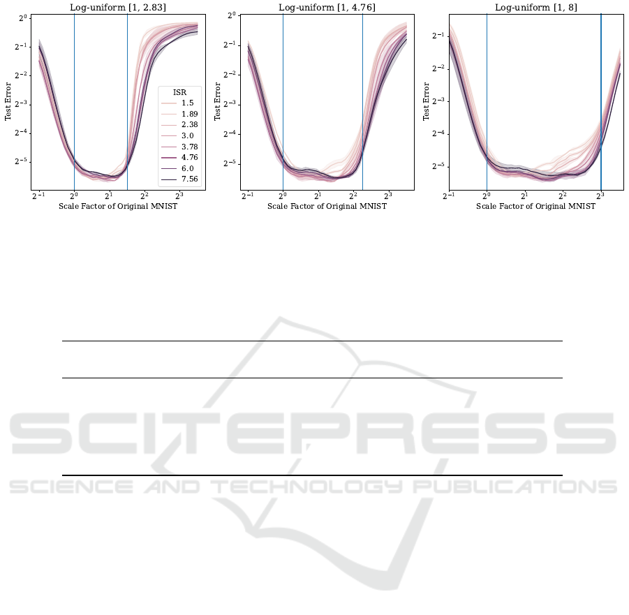
Figure 4: Test Error per data scale for multiple data scale distributions and values for the Internal Scale Range (ISR). Models

with narrow internal scales especially deteriorate in performance in the large-scale region for wide distribution.

Table 2: Learned parameters for the Basis Min Scale σ

basis

and Internal Scale Range (ISR) compared to the conﬁguration of

the best-performing model with ﬁxed internal scales on different ranges of the log-uniform data scale distribution. Apart from

the log-uniform distribution with boundaries [1, 2.83], the learned scale parameters σ

basis

and ISR follow a similar pattern as

the manually found scale parameters. The test error of our scale-learning method is also comparable to the best-performing

models with ﬁxed scales.

Data Scale

Distribution

Scale

Learning

basis

ISR Test Error

Log-uniform [1,2.83] ✓ 1.96 ± 0.081 3.390 ± 0.545 2.291 ± 0.067

✗ 2 2.34 2.239 ± 0.060

Log-uniform [1,4.76] ✓ 2.001 ± 0.063 3.321 ± 0.024 2.510 ± 0.084

✗ 2 4.76 2.503 ± 0.045

Log-uniform [1, 8.00] ✓ 1.943 ± 0.064 4.196 ± 0.159 2.872 ± 0.070

✗ 2 5.35 2.805 ± 0.028

1. Learning the ﬁrst scale (σ

basis

) and the ISR using

the parameterisation from Eq. 5 (Ours)

2. Learning the ﬁrst scale (σ

basis

) and the individual

spacings between subsequent scales

3. Learning the individual scales directly, based on

(Yang et al., 2023) but without deﬁning intervals

the internal scales adhere to.

Table 4 shows the parameterisation methods, the clas-

siﬁcation error and the variation in the learned internal

scales. Unlike shown in (Yang et al., 2023) directly

learning the scales without constraints between the in-

ternal scales does not lead to internal scales converg-

ing to the same value. The methods do not vary sig-

niﬁcantly in performance for the log-uniform distribu-

tion between [1, 2.83] and [1, 4.76] but this changes

when training on wider distributions. All methods

adjust the scales somewhat to account for the wider

scale distribution but our method of learning the In-

ternal Scale Range (ISR) is more stable and achieves

signiﬁcantly better test Error.

4.3 Comparing Baselines

We compare our scale-learning ability against exist-

ing scale-equivariant baselines by evaluating on the

MNIST-Scale (Kanazawa et al., 2014) dataset. We

reuse the code provided in DISCO (Sosnovik et al.,

2021) to compare our results to a baseline CNN and

other methods that take into account scale variations

such as SI-ConvNet (Kanazawa et al., 2014), SS-

CNN (Ghosh and Gupta, 2019), SiCNN (Xu et al.,

2014b), SEVF (Marcos et al., 2018), DSS (Worrall

and Welling, 2019), SESN (Sosnovik et al., 2019) and

DISCO (Sosnovik et al., 2021). All methods adopt

the same training strategy apart from our scale learn-

ing method having a different learning rate scheduler

for its scale parameters.

We also compared our Internal Scale Range based

parameterisation with other parameterisations such

as: learning the individual spacings between inter-

nal scales and learning the scales directly. Learning

the scale directly is similar to the approach taken by

(Yang et al., 2023) but without deﬁning intervals the

internal scales have to adhere to.

Scale Learning in Scale-Equivariant Convolutional Networks

571

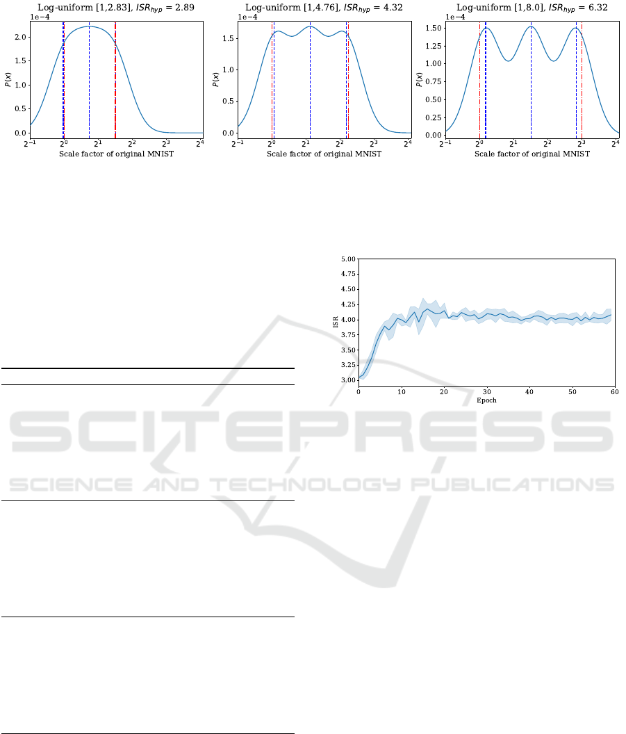
Figure 5: Results of combined optimisation of tolerance hypothesis models and three log-uniform data scale distributions.

The blue dashed line indicates the proposed internal scales, while the continuous blue line represents the tolerance hypothesis

for a speciﬁc data scale distribution. The red dashed lines indicate the boundaries of the loguniform distribution. The result

of ﬁtting the tolerance model results in increasing ISR

hyp

similar to results best performing ISRs found for each data scale

distribution in Fig. 3.

Table 3: Mean and standard deviation of learned scale pa-

rameters (σ

basis

, ISR) and Test Error for different initiali-

sation of σ

basis

and ISR for log-uniform data scale distri-

bution between [1, 2.83], [1, 4.76] and [1, 8]. Learned σ

basis

and ISR values are highly dependent on the values they are

initialised on. Initialisation with a large ISR for a wide data

scale distribution leads to signiﬁcantly lower test error than

initialisation at a low ISR.

Init σ

basis

Init ISR Learned σ

basis

Learned ISR Test Error

Data Scale Distribution: Log-uniform [1,2.83]

1 1.5 1.268 ± 0.061 2.609 ± 0.269 2.487 ± 0.108

3.0 1.236 ± 0.139 3.300 ± 0.082 2.357 ± 0.024

6.0 1.313 ± 0.102 4.350 ± 0.396 2.309 ± 0.021

2 1.5 1.810 ± 0.057 2.405 ± 0.167 2.260 ± 0.025

3.0 1.973 ± 0.079 3.635 ± 0.647 2.368 ± 0.055

6.0 1.994 ± 0.012 5.336 ± 0.283 2.359 ± 0.097

4 1.5 2.778 ± 0.092 2.521 ± 0.199 2.421 ± 0.050

3.0 2.703 ± 0.081 3.817 ± 0.245 2.483 ± 0.089

6.0 2.832 ± 0.001 5.211 ± 0.416 2.420 ± 0.124

Data Scale Distribution: Log-uniform [1, 4.76]

1 1.5 1.294 ± 0.110 3.462 ± 0.410 3.033 ± 0.130

3.0 1.253 ± 0.070 3.829 ± 0.126 2.762 ± 0.087

6.0 1.331 ± 0.091 4.612 ± 0.188 2.727 ± 0.101

2 1.5 1.931 ± 0.068 2.932 ± 0.169 2.767 ± 0.128

3.0 1.975 ± 0.060 3.309 ± 0.092 2.527 ± 0.120

6.0 2.041 ± 0.092 4.882 ± 0.007 2.501 ± 0.157

4 1.5 2.515 ± 0.038 3.093 ± 0.157 2.648 ± 0.073

3.0 2.587 ± 0.040 3.638 ± 0.169 2.575 ± 0.070

6.0 2.803 ± 0.098 5.662 ± 0.204 2.709 ± 0.078

Data Scale Distribution: Log-uniform [1, 8.00]

1 1.5 1.450 ± 0.130 3.767 ± 0.171 3.087 ± 0.173

3.0 1.275 ± 0.076 4.158 ± 0.123 3.131 ± 0.179

6.0 1.331 ± 0.097 5.423 ± 0.529 3.087 ± 0.178

2 1.5 1.755 ± 0.156 3.444 ± 0.025 3.010 ± 0.198

3.0 1.982 ± 0.068 4.095 ± 0.078 2.921 ± 0.082

6.0 2.079 ± 0.061 5.053 ± 0.375 2.745 ± 0.012

4 1.5 2.453 ± 0.151 3.466 ± 0.216 2.935 ± 0.036

3.0 2.607 ± 0.078 4.401 ± 0.343 2.803 ± 0.085

6.0 2.655 ± 0.044 5.268 ± 1.071 2.957 ± 0.140

As can be seen from Table 5, the performance

of the scale learning approaches are very comparable

with SESN (Sosnovik et al., 2019) without learnable

scales. All three scale-learning approaches achieve

test error performance within 1 standard deviation of

SESN with ﬁxed scales. The learned scales, found

in Table 6, are consistently more spread out than the

default scales used in SESN (Sosnovik et al., 2019)

Figure 6: ISR parameter overtime for run initialised with

basis

= 2, ISR = 3 on log-uniform distribution with bound-

aries [1,8]. After around 20 epochs, the learnable ISR sta-

bilises while the value for the ISR of the best-performing

model is signiﬁcantly larger.

especially when scale data augmentation is used.

5 DISCUSSION

We have shown to be able to learn the internal scales,

but the problem of choosing the number of internal

scales remains an issue. For wide scale distribution,

wide internal scales achieve the best performance.

However, if the models were truly scale-equivariant,

the resulting test error would be similar to the test

error for the log-uniform data scale distribution be-

tween 1 and 2.83. More speciﬁcally, if the spacing

between the internal scales is too large the implied

scale-equivariance over the entire range of the inter-

nal scales does not hold up. The model again needs

to learn duplicate ﬁlters to cover the entire data scale

range. This hypothesis also matches up with our In-

ternal Scale tolerance model seen in Fig. 5, which

shows dips in between internal scales. We expect that

increasing the number of internal scales restores the

scale equivariance over the entire scale group with the

downside of reduced computational efﬁciency.

VISAPP 2024 - 19th International Conference on Computer Vision Theory and Applications

572

Table 4: Mean and standard deviation of learned scales and Test Error of different parameterisations for multiple log-uniform

distributions with internal scales initialised as [2.0, 3.46, 6.0]. Learning the ISR leads to more stable learned internal scales

and better performance for wide distributions further away from the initialised scales.

Data Scale

Distribution

Parameterisation Scale 1 Scale 2 Scale 3 Test Error

Log-uniform [1, 2.83] Direct 1.965 ± 0.047 3.500 ± 0.193 6.235 ± 0.497 2.321 ± 0.095

Individual Spacing 1.967 ± 0.079 3.591 ± 0.329 6.930 ± 1.374 2.285 ± 0.038

ISR 1.960 ± 0.081 3.608 ± 0.435 6.672 ± 1.311 2.291 ± 0.067

Log-uniform [1, 4.76] Direct 1.865 ± 0.046 3.357 ± 0.105 6.450 ± 0.049 2.554 ± 0.093

Individual Spacing 1.996 ± 0.013 3.626 ± 0.158 6.830 ± 0.167 2.565 ± 0.061

ISR 2.001 ± 0.063 3.647 ± 0.127 6.647 ± 0.255 2.510 ± 0.084

Log-uniform [1, 8.00] Direct 1.689 ± 0.109 3.262 ± 0.107 6.997 ± 0.282 3.057 ± 0.015

Individual Spacing 1.902 ± 0.085 3.648 ± 0.165 8.093 ± 0.229 3.007 ± 0.049

ISR 1.943 ± 0.063 3.977 ± 0.053 8.145 ± 0.057 2.872 ± 0.070

Table 6: Learned scale parameters of our model on MNIST-Scale compared to values chosen in SESN (Sosnovik et al., 2019).

The ”+” denotes the use of data scale augmentation. The learned scales of all scale learning methods are much wider than the

initialised scales in SESN (Sosnovik et al., 2019) and DISCO (Sosnovik et al., 2021), especially when scale data augmentation

is used.

Model Scale 1 Scale 2 Scale 3 Scale 4

SESN 1.5 1.89 2.38 3

DISCO 1.8 2.27 2.86 3.6

Ours (Learn ISR) 1.390 ± 0.016 1.890 ± 0.061 2.572 ± 0.164 3.503 ± 0.338

Ours (Learn Spacing) 1.390 ± 0.011 1.930 ± 0.099 2.614 ± 0.300 3.776 ± 0.600

Ours (Learn Scales Directly) 1.375 ± 0.008 1.889 ± 0.054 2.383 ± 0.044 3.297 ± 0.086

Ours (Learn ISR)+ 1.381 ± 0.013 2.066 ± 0.012 3.092 ± 0.038 4.627 ± 0.095

Ours (Learn Spacing)+ 1.373 ± 0.013 1.859 ± 0.069 2.847 ± 0.091 4.646 ± 0.306

Ours (Learn Scales Directly)+ 1.360 ± 0.014 1.741 ± 0.062 2.485 ± 0.050 3.775 ± 0.083

Table 5: Classiﬁcation error of Vanilla CNN and other

methods that take into account scale variations in the data.

The error is reported for runs with and without data scale

augmentation, the ”+” denotes the use of data scale augmen-

tation. Learnable scale approaches perform on par with the

non-learnable scale baseline SESN (Sosnovik et al., 2019).

Model MNIST-Scale MNIST-Scale+ # Params.

CNN 2.02 ± 0.07 1.60 ± 0.09 495k

SiCNN 2.02 ± 0.14 1.59 ± 0.03 497k

SI-ConvNet 1.82 ± 0.11 1.59 ± 0.10 495k

SEVF 2.12 ± 0.13 1.81 ± 0.09 495k

DSS 1.97 ± 0.08 1.57 ± 0.09 475k

SS-CNN 1.84 ± 0.10 1.76 ± 0.07 494k

SESN (Hermite) 1.68 ± 0.06 1.42 ± 0.07 495k

DISCO 1.52 ± 0.06 1.35 ± 0.05 495k

Ours (Learn ISR) 1.72 ± 0.05 1.44 ± 0.09 495k

Ours (Learn Spacings) 1.70 ± 0.10 1.50 ± 0.08 495k

Ours (Learn Scales Directly) 1.74 ± 0.06 1.50 ± 0.08 495k

Another difﬁculty of learning the scales is the ini-

tialisation of the internal scales. We have found that

the initialisation of the internal scales has a large im-

pact on the learned scales and as a result the perfor-

mance. However, we do expect that this can be re-

solved by tuning the training procedure.

In addition, our method adds a signiﬁcant com-

putational overhead since it has to reconstruct the dy-

namic ﬁlter basis functions on each step instead of be-

ing able to reuse the ﬁxed multi-scale basis. However,

hyperparameter optimisation of the scale parameters

would take signiﬁcantly longer.

Learnable scales did not add signiﬁcant gains for

classiﬁcation but for other tasks with larger scale-

variations the importance of choosing internal scales

becomes more important. We anticipate that the abil-

ity to learn the internal scales is especially beneﬁcial

in more complicated scenarios with more complicated

data scale distributions, like a Normal distribution. To

learn the internal scales for more advanced data scale

distributions it might be essential to ﬁnd a way to ad-

ditionally learn or adapt the number of internal scales

based on a heuristic.

ACKNOWLEDGMENT

This project is supported in part by NWO (project

VI.Vidi.192.100).

REFERENCES

Benton, G. W., Finzi, M., Izmailov, P., and Wilson, A. G.

(2020). Learning invariances in neural networks.

Scale Learning in Scale-Equivariant Convolutional Networks

573

CoRR, abs/2010.11882.

Deng, L. (2012). The mnist database of handwritten digit

images for machine learning research. IEEE Signal

Processing Magazine, 29(6):141–142.

Farabet, C., Couprie, C., Najman, L., and LeCun, Y.

(2013). Learning hierarchical features for scene la-

beling. IEEE Transactions on Pattern Analysis and

Machine Intelligence, 35(8):1915–1929.

Florack, L. M., ter Haar Romeny, B. M., Koenderink, J. J.,

and Viergever, M. A. (1992). Scale and the differen-

tial structure of images. Image and Vision Comput-

ing, 10(6):376–388. Information Processing in Medi-

cal Imaging.

Ghosh, R. and Gupta, A. K. (2019). Scale steerable ﬁlters

for locally scale-invariant convolutional neural net-

works. CoRR, abs/1906.03861.

Kanazawa, A., Sharma, A., and Jacobs, D. W. (2014). Lo-

cally scale-invariant convolutional neural networks.

CoRR, abs/1412.5104.

Kullback, S. and Leibler, R. A. (1951). On Information and

Sufﬁciency. The Annals of Mathematical Statistics,

22(1):79 – 86.

Lindeberg, T. (2020). Scale-covariant and scale-invariant

gaussian derivative networks. CoRR, abs/2011.14759.

Lindeberg, T. and Eklundh, J.-O. (1992). Scale-space pri-

mal sketch: construction and experiments. Image and

Vision Computing, 10(1):3–18.

Marcos, D., Kellenberger, B., Lobry, S., and Tuia, D.

(2018). Scale equivariance in cnns with vector ﬁelds.

CoRR, abs/1807.11783.

Naderi, H., Goli, L., and Kasaei, S. (2020). Scale equiv-

ariant cnns with scale steerable ﬁlters. In 2020 In-

ternational Conference on Machine Vision and Image

Processing (MVIP), pages 1–5.

Pintea, S. L., Tomen, N., Goes, S. F., Loog, M., and van

Gemert, J. C. (2021). Resolution learning in deep con-

volutional networks using scale-space theory. CoRR,

abs/2106.03412.

Saldanha, N., Pintea, S. L., van Gemert, J. C., and Tomen,

N. (2021). Frequency learning for structured cnn ﬁl-

ters with gaussian fractional derivatives. BMVC.

Sosnovik, I., Moskalev, A., and Smeulders, A. W. M.

(2021). DISCO: accurate discrete scale convolutions.

CoRR, abs/2106.02733.

Sosnovik, I., Szmaja, M., and Smeulders, A. W. M.

(2019). Scale-equivariant steerable networks. CoRR,

abs/1910.11093.

Sun, Z. and Blu, T. (2023). Empowering networks with

scale and rotation equivariance using a similarity con-

volution.

Tomen, N., Pintea, S.-L., and Van Gemert, J. (2021). Deep

continuous networks. In International Conference on

Machine Learning, pages 10324–10335. PMLR.

Worrall, D. and Welling, M. (2019). Deep scale-spaces:

Equivariance over scale. In Wallach, H., Larochelle,

H., Beygelzimer, A., d'Alch

e-Buc, F., Fox, E., and

Garnett, R., editors, Advances in Neural Information

Processing Systems 32, pages 7364–7376. Curran As-

sociates, Inc.

Xu, Y., Xiao, T., Zhang, J., Yang, K., and Zhang, Z. (2014a).

Scale-invariant convolutional neural networks. CoRR,

abs/1411.6369.

Xu, Y., Xiao, T., Zhang, J., Yang, K., and Zhang, Z.

(2014b). Scale-invariant convolutional neural net-

works. CoRR, abs/1411.6369.

Yang, Y., Dasmahapatra, S., and Mahmoodi, S. (2023).

Scale-equivariant unet for histopathology image seg-

mentation.

Zhu, W., Qiu, Q., Calderbank, A. R., Sapiro, G., and

Cheng, X. (2019). Scale-equivariant neural net-

works with decomposed convolutional ﬁlters. CoRR,

abs/1909.11193.

APPENDIX

Dataset Description

Dynamic Scale MNIST. The Dynamic Scale

MNIST pads the original 28x28 images from the

MNIST dataset (Deng, 2012) to 168x168 pixels and

then on initialisation of the dataset, an independent

scale for each sample is drawn from the chosen scale

distribution. Only scales e larger than 1 are sampled

during training time to prevent the inﬂuence of in-

formation loss which occurs when downsampling the

data. Since each digit is upsampled upon accessing no

additional storage is needed to use this dataset for var-

ious scale distributions. After initialisation the dataset

is normalised.

Additionally, this dataset can also be used to eval-

uate across a range of scales by sampling each test

digit individually on multiple scales. The scales to

evaluate are rounded to the nearest half-octave of 2.

The number to evaluate is determined by the range of

octaves times 10. Thus for Fig. 4, 45 scales are sam-

pled between 2

−0.5

and 2

3.5

in a logarithmic manner.

The underlying MNIST dataset (Deng, 2012) is split

into 10k training samples, 5k validation samples, and

50k test samples and 3 different realisations are gen-

erated and ﬁxed.

MNIST-Scale The images in the MNIST-Scale

dataset are rescaled images of the MNIST dataset

(Deng, 2012). The scales are sampled from a Uni-

form distribution in the range of 0.3 - 1.0 of the orig-

inal size and padded back to the original resolution

of 28x28 pixels. The dataset is split into 10k training

samples, 2k validation samples and 50k test samples

and 6 realisations are made.

VISAPP 2024 - 19th International Conference on Computer Vision Theory and Applications

574