Evolutionary-Based Ant System Algorithm to Solve the Dynamic Electric

Vehicle Routing Problem

Simon Caillard and Rachida Ben Chabane

Laboratory CESI Lineact, 2 all

ee des Foulons, Parc des Tanneries, Strasbourg, France

Keywords:

Dynamic Electric Vehicle Routing Problem, Ant Colony Optimization, Evolutionary Algorithms, Immigrant

Scheme, Memory Based.

Abstract:

This article addresses the Dynamic Electric Vehicle Routing Problem with Time Windows (DEVRPTW) using

a hybrid approach blending genetic and Ant Colony Optimization (ACO) algorithms. It employs an Ant Sys-

tem algorithm (AS) with an integrated memory system that undergoes mutations for solution diversiﬁcation.

Testing on Schneider instances under static and dynamic conditions, with run time of 10 and 3 minutes respec-

tively, reveals promising results. Compared to static solutions, deviations of 8.55% and 2.38% are observed

in vehicle count and total distance. In a dynamic context, the algorithm maintains proximity to static results,

with 10.99% and 4.41% deviations in vehicle count and distance. Instances R1 and R2 present challenges,

suggesting potential improvements in memory and pheromone transfer during re-optimization.

1 INTRODUCTION

The environmental impact of economic and techno-

logical growth, emphasize the role of fossil fuel com-

bustion in greenhouse gas (GHG) emissions and cli-

mate change. The transportation sector, a major fos-

sil fuel consumer, contributed signiﬁcantly to GHG

emissions in the EU. As a response, governments

globally implemented policies to reduce emissions

and fossil fuel use. The EU set ambitious goals to

decrease GHG emissions by 80-95% by 2050 com-

pared to 1990 levels. In last decade, Electric vehi-

cles (EVs) have gained popularity for their environ-

mental beneﬁts, like zero GHG emissions and energy

efﬁciency. Notable companies like FedEx and DHL

have incorporated EVs into their ﬂeets, with examples

of substantial ﬂeet expansions and new deployments.

While EVs offer advantages, they face challenges in-

cluding limited range, longer charging times, higher

costs, and a developing charging infrastructure.

The Vehicle Routing Problem (VRP) involves

ﬁnding efﬁcient routes for a ﬂeet of vehicles to

meet customer demands and has been ﬁrst introduced

by (Dantzig and Ramser, 1959). With time, vari-

ations like Capacitated-VRP, Heterogeneous-Fleet-

VRP, and Time-Dependent-VRP have introduced spe-

ciﬁc constraints (Kumar and Panneerselvam, 2012),

and more recently Electric Vehicle Routing Problems

(EVRP) has emerged (Erdo

gan and Miller-Hooks,

2012). EVRP studies extend VRP concepts, but face

complexity due to limited electric vehicle range and

recharging needs. This introduces challenges like

station placement, recharging policies, and various

charging functions and many works focus on the ex-

tension related to EVRP (Qin et al., 2021; Erdeli

et al., 2019). Nevertheless, the existing methods

primarily address static scenarios, where all data is

known in advance. However, real-world applica-

tions often face dynamic environments. This study

emphasizes the Dynamic Electric VRP (DEVRP), a

more challenging problem that requires not only ﬁnd-

ing optimal solutions quickly but also adapting to

data changes (Mavrovouniotis and Yang, 2015). A

common approach in handling DEVRP involves two

phases (Leal and Silva Junior, 2020): ﬁrst, gener-

ating routes for conﬁrmed clients using static tech-

niques, and second, periodically re-optimizing routes

throughout the working day to adapt the solutions

provided to the arrival of new customers requests.

Many technics have been used to solve (E)VRP

and its variants. The most known to achieve very good

results are the local search, variable neighborhood

search, large neighborhood search, etc. (Erdeli

c et al.,

2019). Among them, we found Ant Colony Optimiza-

tion (ACO) algorithms that can achieve similarly re-

sults (Thymianis et al., 2022). However, ACO are pri-

marily designed for static optimization (Dorigo et al.,

1996), aiming for rapid convergence to a global or

Caillard, S. and Ben Chabane, R.

Evolutionary-Based Ant System Algorithm to Solve the Dynamic Electric Vehicle Routing Problem.

DOI: 10.5220/0012379200003639

Paper published under CC license (CC BY-NC-ND 4.0)

In Proceedings of the 13th International Conference on Operations Research and Enterprise Systems (ICORES 2024), pages 285-293

ISBN: 978-989-758-681-1; ISSN: 2184-4372

285

near-global optimum. A challenge arises in dynamic

optimization scenarios, where residual pheromone

trails from previous environments can bias the pop-

ulation towards the old optimum. This hinders the

tracking of the evolving optimum, making it difﬁcult

for ACO to adapt once it converges on a solution. One

straightforward but often inefﬁcient approach to dy-

namic problems is to treat them as a series of static

instances by resetting pheromone trails and solving

from scratch after each change (Mavrovouniotis and

Yang, 2013). In dynamic environments, ACO algo-

rithms can beneﬁt from prior pheromone trails. When

the current conditions resemble previous ones, these

trails can speed up optimization (Guntsch and Mid-

dendorf, 2002). However, the algorithm needs to be

ﬂexible enough to either integrate the knowledge from

these trails or discard them if they are outdated and

no longer relevant to the new environment. More re-

cently, ACO are combined with local/variable neigh-

borhood search algorithms to enhance quickly their

results (Mao et al., 2020; Wu and Gao, 2023)

Numerous strategies have been put forth and in-

tegrated with ACO to reduce re-optimization time

while efﬁciently preserving output quality. These

strategies fall into several categories: enhancing di-

versity following a dynamic change (Mavrovounio-

tis and Yang, 2013), sustaining diversity throughout

execution (Eyckelhof and Snoek, 2002), memory-

based schemes (Mavrovouniotis and Yang, 2012), hy-

brid/memetic algorithms (Wang et al., 2021) and im-

migrant schemes (Mavrovouniotis and Yang, 2012).

For the last one, a subset of newly generated ants (the

immigrant ants), replace the weakest ants in the cur-

rent population. The approach to generating immi-

grant ants differs. For example, random immigrants

represent random solutions to the problem (Mori

et al., 1996), while elitism- or memory-based immi-

grants present solutions that deviate slightly from the

best solution of a previous environment (Yang, 2008).

This paper particularly delves into immigrant

schemes for the DEVRP, where the immigrant ants

represent a viable VRP solution. The contributions of

this study can be summarized as follows: We extend

EVRPTW into dynamic pickup environment, which

is more practical and propose an Ant System algo-

rithm using evolutionary concept and an immigrant

scheme to solve it. The results are validated through-

out a series of test instances derivated from those of

Solomon, a well-known benchmark. The rest of this

paper is outlined as follows. 2 formally presents the

DEVRP and the structure of a solution. Section 3 de-

scribes the proposed ACO algorithm. Section 4 intro-

duces DEVRP benchmarks, generated from those of

Solomon, and evaluates empirically the performance

of the proposed method. The ﬁnal section concludes

this paper with discussions on future works.

2 FORMALIZATION OF THE

DEVRPTW AND ITS SOLUTION

The formulation of the DEVRPTW proposed in this

paper is based on the one provided by (Schneider

et al., 2014). It can be modeled as a complete directed

graph G = (V

′

,A). V

′

= V ∪ F ∪ {0,N + 1} repre-

sents the set of vertices with V = {1,.. ., N} and F

respectively the set of customers and recharging sta-

tions. Vertices 0 and N + 1 corresponds to the same

depot, and each routes starts at 0 and ends at N + 1.

A = {(i, j) ∈ V

′

|i ̸= j} is the set of arcs. To each arc

is associated a distance d

i, j

and a travel time t

i, j

. To

each vertex i ∈ V

′

is associated a pick-up demand q

, a

service time s

, a time rt

at which the request of cus-

tomer i is know, and a time windows [e

] in which

the service has to start. So, the service cannot start

before e

or after l

, but might end later. We note that

∀i ∈ {0, N + 1} ∪ F, q

= 0, s

= 0 and rt

= 0. In

addition, we note n f

= f ∈ F|min d

i, f

, the nearest

recharge station to customer i. The planning horizon

H = [e

] corresponds to the opening time windows

of the depot, and the recharge stations are generally

available on the entire horizon. There is a set of ve-

hicles U and for each vehicle u, C

and Q

repre-

sent respectively its total loading and battery capac-

ities. When an arc {i, j} ∈ A is traveled by a vehicle,

a quantity of e · d

i, j

of the remaining battery charge

is consumed, with e which corresponds to the con-

stant charge consumption rate. At a recharging sta-

tion, the time required for recharging depends on the

difference between the current charge level and the

battery capacity. This recharging process occurs at a

rate of d which is linear. In other words, the duration

of recharging is inﬂuenced by the initial energy level

of the vehicle upon arrival at the station. The function

(i) allows us to know the remaining battery capac-

ity of vehicle u ∈ U when it arrives at vertex i ∈ V

′

Several constraints and assumptions must be ful-

ﬁlled to ensure a valid solution. They are listed above:

• The sum of the pick-up demands of the customers

visited by a vehicle must not exceed its capacity.

• Each route must starts (vertex 0) and ends (vertex

N + 1) at the depot.

• A customer can be visited only during its time

windows availability.

• Each client must be served at most once.

ICORES 2024 - 13th International Conference on Operations Research and Enterprise Systems

286

• The pick-up demand fulﬁllment of each customer

must be guarantee.

• The battery level of each vehicle must never falls

below 0.

• After leaving the depot and each charging station,

the battery is brought back to full charge.

• The ﬂow conservation constraints must be re-

spected: the number of incoming arcs is equal to

the number of outgoing arcs.

• The time feasibility must be respected for arcs

leaving a vertex: when considering two vertices, i

and j, the arrival time at vertex i, increased by the

combined travel time from i to j and service du-

ration (or recharge time) at i, must be shorter than

the arrival time at vertex j.

• There are at most as many simultaneous routes as

there are vehicles.

As mentioned earlier, there are different types of dy-

namics, with the most common, and the one studied in

this paper, being the arrival of new customer requests

during the day. Therefore, customer requests are not

fully known in advance, but arrive dynamically during

the parcel retrieval process. Consequently, to incorpo-

rate these new requests, the routes must be promptly

re-planned, either immediately or every xx minutes

in the case of continuous or periodic re-optimization.

Then, the DEVRPTW is considered as a sequence of

instances which slightly differ from each other.

A common approach for addressing DEVRPTW

is known as the ”least-commitment strategy.” This

strategy hinges on two distinct scenarios regarding

interaction with the planned solution. The problem

is deemed preemptive if, upon receiving a new cus-

tomer request, a vehicle can divert from its current

route to serve the new customer. In contrast, the non-

preemptive approach, adopted in this paper, means

that once a vehicle is en route to its next destination,

it must adhere strictly to this trajectory, without al-

lowance for deviations or interruptions at this stage of

the route. A crucial aspect of dynamic routing prob-

lems is establishing a metric to quantify the level of

dynamism in the problem: the degree of dynamism. It

is a value within [0,1], deﬁned as the ratio between the

quantity of dynamic customers (those that are known

after e

) and the overall number of customer. If the

degree of dynamism is 0, the instance is static and

then all customer are already known before e

To help the general comprehension of this papers,

additional notations are introduced because of the dy-

namic context. When the periodic re-optimization oc-

curs, a new instance must be resolved, in which one

or more new clients has arrived during the horizon H.

So, it is necessary to track the position of the vehi-

cles over time: we introduce functions pos(u,h) and

time(u,i). The ﬁrst one returns the vertex i at which

vehicle u stands at time h. The second gives the time h

at which vehicle u ∈ U visits i. These functions allow

us to compute the couple avail

= (h,i) and know-

ing precisely where and when each vehicle will be

available when the periodic re-optimization occurs,

because we are in a dynamic and non-preemptive con-

text.

A solution to the DEVRPTW can be expressed as

a sequence of routes followed by a vehicle. A route

is deﬁned as sequence of vertices (customers and/or

recharge stations) starting and ﬁnishing respectively

at vertices 0 and N + 1. Let Π = r

,. .. ,r

|Π|

be a

solution to the DEVRPTW. ∀r ∈ Π, r ⊆ V

′

, and r =

0,. .. ,N +1 is a path in G representing a vehicle route.

To asses the quality of a solution Π, we use the

function (F)

tot

, given by equation (1). The objective

is to determine a solution for which the number of un-

visited customers, the number of routes and the total

distance traveled are minimized.

tot

(Π) = F

cust

+ F

rte

(Π) + F

dist

(Π) (1)

With F

cust

, F

rte

(Π) and F

dist

(Π) that represent re-

spectively the number of unvisited customer, the num-

ber of routes and the total distance traveled for the

solution Π. These objectives are hierarchical, which

means that a solution with no unvisited customers will

be better than another with 1 or more unvisited cus-

tomers and a lower total distance traveled.

Figure 1 shows the graph representation of the

DEVRPTW for a small instance. In this problem

V = {0,1,2, 3,4}, and F = { f

}. Around each ver-

tex, we found the data relating to it. For example, for

vertex 1, q

= 2, s

= 1, rt

= 3, e

= 5 and l

= 10.

Vertex 0/4 is the depot and its interval of availabil-

ity corresponds to its opening hours. f

is a recharge

station which is available on the entire horizon. More-

over, there are 2 vehicles with a capacity of 5, a bat-

tery capacity of 6 and a consumption rate of 1. The

weight on each arc correspond to the travel time and

to the distance between vertex. It is assumed to be

equal to facilitate computation in this example.

At time 0, Π = {{0,2, f

,3, 4}} is a solution to

this instance whose evaluation F

tot

(Π) = 0 +1 + (2 +

3 + 4 +1) = 12. This solution is composed of 1 route

that visits vertices 0, 2, f

, 3 and 4. The vertex 1

is not known at this moment. In details, the vehicle

starts at the depot at time 0 and arrives at vertex 2 at

time 2 (travel time required to go from 0 to 2) and

leave it at time 2 + 2 = 4 (travel time + service time).

Then it visits vertex f

at time 7 and so on. Because

the consumption rate h = 1, the vehicle has consumed

1 · (2 + 3 + 4 + 1) = 10 unit of the battery.

Evolutionary-Based Ant System Algorithm to Solve the Dynamic Electric Vehicle Routing Problem

287

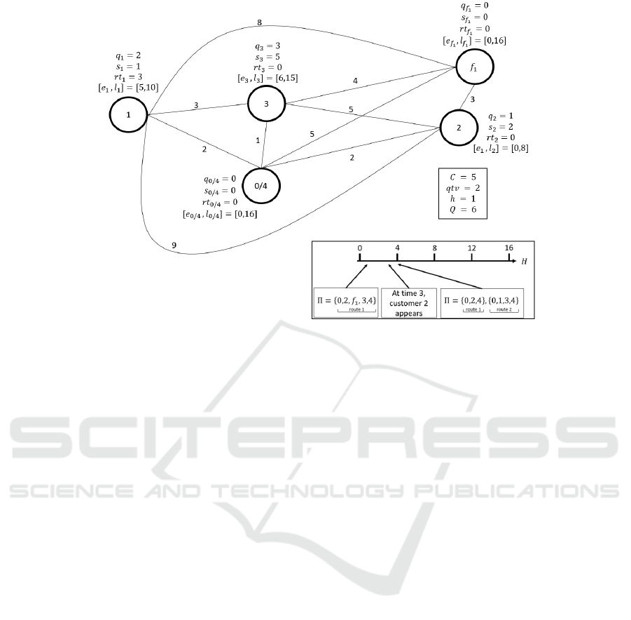
Figure 1: Graph representation of the DEVRPTW and of a solution.

When the periodic re-optimization occurs, cus-

tomer 1 is known. It is arrived at time 3 but is take

into account only at time 4. At this moment, the ve-

hicle on route 1 has ﬁnished to serve client 2. Since

vehicle 1 lacks the necessary battery capacity and re-

quires charging times due to the distance, it won’t be

able to reach customer 1 within its availability win-

dow. In this context, it is necessary to add a route

to serve the customers. Then at time 4, a solution

could be Π = {{0,2, 4},{0, 1,3,4}}. Its evaluation

tot

(Π) = 0 + 2 + ((2 + 2) + (2 + 3 +1)) = 12.

3 EVOLUTIONARY-BASED ANT

SYSTEM

3.1 General Framework

To help the construction of solutions, most of the

ACO algorithms rely on heuristics in addition to

pheromones that store the information about the best

generated solutions. In comparison, evolutionary al-

gorithms form an active population carried over be-

tween iterations using selection methods. In this

study, we propose a population-based ants system

which maintain a population consisting in the best

ants encountered from the start of the algorithm. The

aim is to sustain diversity within this population and

transmit knowledge to the pheromone trails. When

similarities between the population reach a predeﬁned

level, the pheromone trails and the population are par-

tially reset. In order to store the population over each

iteration it: some ants are removed while others are

added, it is imperative to establish a memory M

size M

. Indeed, to constitute the the memory M (i)

of the iteration i, the M

best ants generated at this

iteration are faced in tournament with the set of ants

M (i − 1) which were retained from the previous iter-

ation.

Figure 2 details the general process of our algo-

rithm. While a preset time limit is not reached, at each

iteration: (1) ants build solutions using heuristic and

pheromones information, (2) if the similarity between

the best ant ever encountered and the ants generated

in this iteration exceeds a predeﬁned threshold, both

the pheromone matrix and the currently memorized

population are reset, else the population in memory is

updated through a confrontation between the best ants

generated in this iteration and those currently stored,

(3) some ants in the memory undergo mutations (4)

the ants deleted from the population in this iteration

remove their pheromones, then all the ants in mem-

ory deposit pheromones and (5) if it is time for peri-

odic re-optimization, then the data of the instance are

updated and the pheromones matrix is reinitialized.

At the start of the algorithm, the current time

h = 0, the population at iteration M (0) =

0 and the

matrix of pheromones τ of size V

′

×V

′

, is initialized

at τ

init

= 1/F

tot

(Π

init

), where Π

init

corresponds to a

solution constructed using a greedy heuristic based

on the distance to next customer and taking into ac-

count both the commencement and duration of its

time window. Moreover, for each vehicle u ∈ U,

avail

= (0,0). This last value may differ when the

ICORES 2024 - 13th International Conference on Operations Research and Enterprise Systems

288

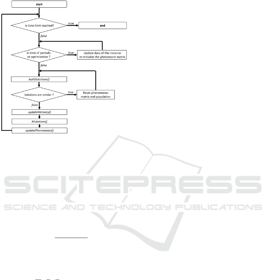
Figure 2: Flowchart of the proposed algorithm.

periodic re-optimization occurs.

3.2 Function buildSolutions()

A set of antQty ants generate solution, starting from

the depot (see the constraints described in section 2).

Each ant built his own solution, selecting the next ver-

tex to visit according to the random proportionality

rule that rely on the probability p

i, j

. This probability

is based on both heuristic and pheromones informa-

tion and is described in equation 2.

i, j

· η

i, j

∑

j∈UN

i, j

· η

i, j

(2)

Where p

i, j

is the probability to visit vertex j when

ant k is located at client i, τ

i, j

represents the exist-

ing pheromone trail on the arc between customers i

and j, η

i, j

, with h

the time at which

the vehicle is scheduled to depart from i, corresponds

to the heuristic information that prioritizes the closest

customers, whose time windows are short and which

will soon close, UN

is the set of available unvisited

neighborhood customers for ant k when it stands on

vertex i: those for which h

+ t

i, j

≤ l

. α and η are

coefﬁcient that specify the relative importance of re-

spectively pheromones and heuristic information. We

note that if a vehicle arrives at a customer j before the

start e

of its time windows, the vehicle wait until this

moment before starting the service of j.

When selecting the next customer would result in

an impractical solution (e.g., exceeding the maximum

vehicle loading or battery capacities), the depot or

a recharge station is selected depending of the con-

straint violated (battery capacity, or loading capacity)

. Note that if the vehicle does not have enough battery

to return to the depot, then the nearest charging station

is selected. A vehicle returning to the depot implies

the start of a new vehicle route. This sequence con-

tinues until all customer demands are met, ultimately

leading to a feasible DEVRPTW solution constructed

by an ant. The quantity of routes in a solution deter-

mines the number of vehicles used.

Taking into account the current customer i, the

previously chosen next customer j, the constraint as-

sociated with battery consumption and the constraint

related to vehicle loading capacity, there are several

scenarios that compel the vehicle to either proceed to

a charging station or return to the depot:

Battery Capacity: there is not enough battery to go

from customer i to j (C

(i) − e · t

i, j

≤ 0), or once

arrived at customer j, there is not enough battery

to reach the nearest charging station n f

(i) −

e · (t

i, j

+ t j, n f

≤ 0). In both cases, the nearest

charging station n f

is selected.

Load Capacity: if the request q

of the next cus-

tomer j leads to the vehicle’s capacity being ex-

ceeded, then the depot N + 1 is selected only if

there are enough remaining battery to reach it,

otherwise the nearest charging station n f

of cur-

rent customer i, is selected. We note that n f

always reachable because of the checks related to

the battery consumption constraint.

An iteration it is concluded once all ants have created

workable solutions, resulting in the generation of a

population P

3.3 Function updateMemory()

Prior to updating the memory, updateMemory()

checks that the algorithm did not converged toward a

local minimum. We can ensure that a local optimum

is reached when the similarities between the best and

worst solutions obtained at a given iteration exceed

a predetermined threshold (for example: 95%). This

behavior means that some pheromones are too high

compared to others, so the algorithm constructs al-

most identical solutions.

If a local optimum is reached, a re-initialisation of

the memory and of the pheromones matrix occur. The

rate ξ(it) is computed. It deﬁnes how close are the so-

lutions generated at this iteration it, thanks to the met-

ric comp(Π

,Π

) which compare solutions pairwise.

This computation of ξ(it) is detailed in equation 3.

Evolutionary-Based Ant System Algorithm to Solve the Dynamic Electric Vehicle Routing Problem

289

ξ(it) =

∑

,Π

∈P

|Π

̸=Π

comp(Π

,Π

)

with

comp(Π

,Π

) = 1



CE(Π

,Π

)

′

| + avg(|Π

|,|Π



(3)

Where CE(Π

,Π

) denotes the shared edges be-

tween solutions Π

and Π

, and avg(|Π

|,|Π

|) rep-

resents the average number of routes for Π

and Π

The closer ξ is to 0, the more similar the solutions are,

and if it is less than an predeﬁned threshold M

reset

a re-initialisation of the pheromone matrix and the

memory is triggered: all the pheromones of τ are set

to τ

init

and M

If the re-initialisation is not triggered, then the

memory is updated. This process is done using a sys-

tem of tournament in which the solutions of P

and

it−1

confront each other. From P

∪M

it−1

, function

updateMemory() (see algorithm 1) randomly selects

couple of solutions that are compared using our

objective function F

tot

. This function ensures a new

memory M

for the iteration it and del

, a set of so-

lutions that are no longer in the memory and which

will be used when updating the pheromones of this

iteration it.

Require: M

it−1

, P

Ensure: M

, del

1: del

←

0, M

←

2: ξ(it) ← computeXi(P

)

3: if ξ(it) ≤ M

reset

then

4: del

← M

it−1

, M

←

5: else

6: duo ←

0, bu f f er ← M

it−1

∪ P

7: while bu f f er ̸=

0 do

8: (Π

,Π

) ← randomChoiceTwice(bu f f er)

9: bu f f er ← bu f f er \ {Π

∪ Π

}

10: duo ← duo ∪ (Π

,Π

)

11: end while

12: for all (Π

,Π

) ∈ duo do

13: if F

tot

(Π

) ≤ F

tot

(Π

) then

14: M

← Π

, del

← Π

15: else

16: M

← Π

, del

← Π

17: end if

18: end for

19: del

← del

∩ M

it−1

20: end if

21: return M

, del

Algorithm 1: updateMemory().

3.4 Function mutations()

In the traditional approach, mutations occur on some

solutions of the current population by partially mod-

ify them (e.g two customers of two distinct routes are

swapped). In the DEVRPTW, this approach is dif-

ﬁcult to implement while maintaining feasibility be-

cause of the to numerous constraints (notably that

of time windows and battery). To address this is-

sue, mutations are implemented not by partially mod-

ifying solutions, but by directly altering the memory

through the replacement of some solutions. Tak-

ing into account the framework of our population-

based ant system (see ﬁgure 2), prior to updating the

pheromone trails, a total of ⌊M

/4⌋ greedy random-

ized solutions are generated to substitute the poor-

est ants in M

. This is designed to excel in dy-

namic environments characterized by swift and sub-

stantial changes, thanks to the diversity introduced by

the random solutions. This is particularly effective

when dealing with dissimilar changing environments,

as increasing diversity at random proves superior to

knowledge transfer, a conclusion conﬁrmed in the dy-

namic traveling salesman problem.

A greedy random solution is generated using a

similar process to the one used in function buildSolu-

tions(), except the pheromone value that are not con-

sidered to select the next customer. In details, if an

ant k is chosen for replacement in M

its correspond-

ing solution Π

0. Ant k must then construct a

new solution using a random greedy heuristic. To do

this, it starts from the depot and randomly selects the

next customer j ∈ UN

to visit while located at node i

with a 20% probability. Otherwise, it employs a ran-

dom proportionality rule solely based on the heuris-

tic η

i, j

(meaning pheromones are not used) to choose

the next customer j to visit from UN

. As reminder,

corresponds to the unvisited customers for which

i, j

≤ l

with h

the time at which ant k leave ver-

tex i. As reminder, just as function builSolutions(),

if ant k arrives at customer j before the start of its

time windows, it wait until e

to start the service of j.

Furthermore, if the chosen next customer leads to an

infeasible solution due to vehicle loading or battery

capacity constraints, either the depot or a recharge

station is selected depending on which constraint is

violated. This rules are the same as those detailed in

subsection 3.2.

3.5 Function updatePheromones()

The distinctive feature of our population-based ant

system used in this study, in contrast to conventional

ACO algorithms, relies on the integration of a mem-

ory used in conjunction with the pheromone matrix.

At the end of an iteration, each solution Π ∈ M

are

allowed to deposit pheromones according to equation

4, whit r that represent a route in solution Π and τ

max

the maximum value reachable for the pheromones.

ICORES 2024 - 13th International Conference on Operations Research and Enterprise Systems

290

i, j

= min(τ

max

, τ

i, j

tot

(Π)

) ∀r ∈ Π (4)

In addition, a negative pheromone update is ap-

plied to each solution Π in del

: the solution that was

in M

it−1

but that are not in M

, according to equation

5, whit r that represent a route in solution Π, τ

init

the

initial value of the pheromones, and dep

the number

of times that solution Π has been allowed to deposit

pheromone.

i, j

= max(τ

init

, τ

i, j

− dep

tot

(Π)

) ∀r ∈ Π (5)

If it is the time for periodic re-optimization, a sec-

ond update of the pheromones occurs, in which all the

pheromones in the matrix τ are decreased by a ﬁxed

amount, as described in equation 6.

i, j

= max(τ

init

, τ

i, j

−

max

− τ

init

∀(i, j) ∈ τ (6)

4 EXPERIMENTATION

To asses the effectiveness of our algorithm, we need

to test it on dedicated instances. Fortunately, it ex-

ists instances in the state of the art that are com-

mon to both the Electric-VRPTW (EVRP) and the

Dynamic-VRPTW (DVRP): the Solomon benchmark

(Solomon, 1984) for the VRPTW. The Solomon’s in-

stance are categorized into three classes based on the

spatial arrangement of customer locations: random

customer distribution (R), clustered customer distri-

bution (C), and a combination of both (RC). Within

these groups, R1, C1, and RC1 have a relatively short

scheduling horizon, typically demanding more vehi-

cles to cater to all customers compared to R2, C2, and

RC2, which possess a longer scheduling horizon. Ad-

ditionally, instances within a group vary in terms of

time window density and time window width.

In (Schneider et al., 2014), the author details how

he has generated a set of 56 instances with 100 cus-

tomers for the EVRP, which are based on those of

Solomon. He adds a recharge station at the depot

and randomly places an additional 20 stations. How-

ever, he restricts the potential locations to ensure the

creation of viable and relevant instances, within each

customer can be reached from the depot using a max-

imum of two distinct recharging stations. The bat-

tery capacity is determined based on two factors: (1)

the charge needed to cover 60% of the average route

length of the best-known solution for the correspond-

ing VRPTW instance, and (2) twice the charge re-

quired to travel the longest distance between a cus-

tomer and a station. Moreover, the consumption rate

is set to 1.0 for simplicity. The recharging rate is

adjusted so that a full recharge takes three times the

average customer service time of the respective in-

stance. Finlay he has adjusted the customers time

windows to ensure that instances remain feasible.

To introduce a dynamic element to the Solomon

benchmarks, the authors in (Yang et al., 2017) pro-

pose the following method: a certain percentage of

nodes are only disclosed during the course of the

working day. A degree of dynamism of X% indicates

that each customer vertex i has a probability of X%

to receive a non-zero available time (rt

̸= 0), repre-

senting the moment when the request is known. This

available time is generated within the interval [0, ¯e

where ¯e

= min(e

i−1

). t

i−1

represents the departure

time from the last vertex visited before i in the best

known solution.

To generate our instances, we use the method

proposed by Yang (Yang et al., 2017) to the bench-

marks given by Schneider (Schneider et al., 2014) for

which we consider its results as the best known so-

lutions. The results given in the section are divided

in two categories: when the degree of dynamism

X = 0 (the instances are static), and when X = 0.5

which mean that at most 50% of the customers re-

quests are known during the course of the working

day. For both categories, the instances were run 10

times on single thread with a Ryzen 5600U proces-

sor @2.30GHZ with 16GB of RAM on a computer

running Windows 11. The algorithm proposed has

been implemented using Python 3.11 and the follow-

ing empirically determined values of the parameters

are used: α = 2, β = 4, M

= 8, M

reset

= 0.1 and

max

= τ

init

+ M

· F

tot

(Π

best

), with Π

best

that corre-

sponds to the best solution encountered during the

process of the algorithm (τ

max

is therefore dynamic).

The number of ants antQty = 15.

Table 1 gives the result of our population-based

ant system in a static context (all customers are known

at the start of the algorithm), and are compared to the

best results given by Schneider in (Schneider et al.,

2014). For our algorithm, each run has a duration of

7 minutes. For those of Schneider, only a meantime

in given which is around 16 minutes. Column Family

gives the category of the instances tested (e.g. C1,

C2, RC1 and so), column Schneider shows the best

results obtained by Schneider, while column EB-AS

gives the mean of our objective function over 10 runs

of each instances of the corresponding family. For

both, columns m and f give respectively the number

of vehicles and the total distance traveled.

The observations reveal that the outcomes closely

align with Schneider’s results. There exists a dis-

crepancy of 8.55% in the number of vehicles utilized,

and a margin of 2.38% favors Schneider in terms of

Evolutionary-Based Ant System Algorithm to Solve the Dynamic Electric Vehicle Routing Problem

291

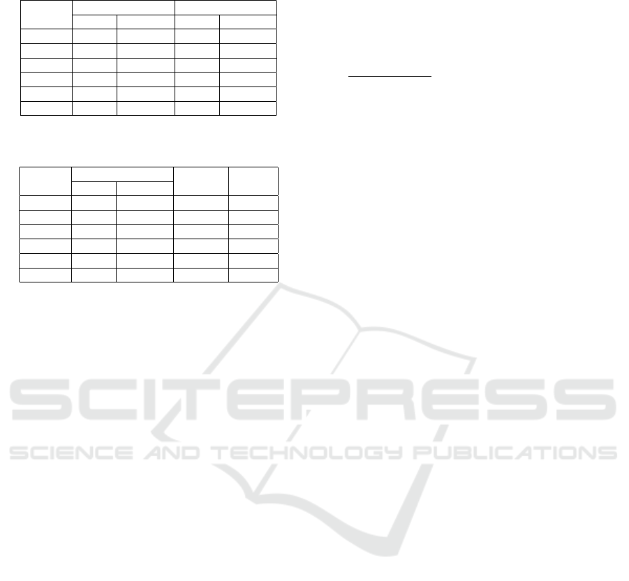
Table 1: Results of Schneider and EB-AS for DEVRPTW

instances in a static context.

Family

Schneider EB-AS

m f m f

C1 10.66 1048.11 10.91 1054.98

C2 4 640.79 4.42 669.51

R1 12.83 1259.29 12.92 1266.02

R2 2.63 800.41 3.05 817.26

RC1 13.12 1409.25 13.12 1488.46

RC2 3.125 1145.37 4,07 1167.14

Table 2: Comparison between dynamic and static results

obtained by EB-AS for DEVRPTW instances.

Family

EB-AS dynamic

∆ m ∆ f

m f

C1 11.42 1106.45 4.39% 4.57%

C2 4.75 699.06 4.30% 4.07%

R1 14.72 1347.12 12.26% 5.84%

R2 4.86 884.28 35.27% 7.50%

RC1 13.79 1518.06 4.79% 1.89%

RC2 4,31 1197.34 4.92% 2.58%

the overall distance covered. Notably, all customers

were successfully served, leading to the omission of

the objective function component pertaining to un-

served customers. However, it is important to note

that Schneider’s execution time is more than 1.5 times

longer than ours, which could account for this varia-

tion.

Table 2 gives the result of our population-based

ant system in a dynamic context, with a degree of

dynamism X = 0.5 (only half of the customers are

known at the start of the algorithm), and are com-

pared to our results in a static context. The periodic

re-optimization occurs every 5 minutes. This implies

that for a Schneider instance with a time horizon of

H = [0, 1000], assuming an 8-hour workday, periodic

re-optimization takes place approximately every 11

time units. As a result, if new clients arrive within

this 10-unit time window, the algorithm is restarted,

taking into account the new clients, vehicle positions,

battery status, and remaining charging capacities. The

initial optimization carried out before the start of the

workday is allowed a maximum run time of 5 min-

utes, while subsequent optimizations run for a max-

imum of 2 minutes to facilitate the transmission of

the routes updates to the vehicles. Column Family

gives the category of the instances tested (e.g. C1,

C2, RC1 and so), column EB-AS dynamic gives the

average of our objective function over 10 runs of each

instances of the corresponding family: columns m and

f give respectively the number of vehicles and the to-

tal distance traveled. Columns ∆ m and ∆ f express

the gap (in percent) between the results of EB-AS in a

dynamic and static context.

We observe average results very close to those in

a static context, with a gap of 10.99% and 4.41% in

terms of quantity of vehicles used and the total dis-

tance traveled, respectively. Moreover, for a speciﬁc

instance, if we measure the closeness of the solu-

tions respectively obtained in a static and dynamic

context using the the metric comp(Π

stat

,Π

dyn

) =



CE(Π

stat

,Π

dyn

)

′

|+avg(|Π

|,|Π



(described in equation 3), with

stat

and Π

dyn

respectively the solutions obtained in

a static and dynamic context. We found an average

of 83% similarities between static and dynamic solu-

tions.

This demonstrates that the algorithm is able to

do good decisions even while it doesn’t have prior

knowledge of all the customers to be served during

the workday. However, we do notice a larger devia-

tion in the R1 and R2 instance families, where cus-

tomer positions are random. This can be explained

by our heuristic which considers the duration and re-

maining time in the customer’s time window. Thus,

vehicles already on the road may stray far from the

depot, necessitating the dispatch of additional vehi-

cles during periodic re-optimization, as none of them

can meet the demand of new customers in a timely

manner.

5 CONCLUSIONS

In this article, we address the DEVRPTW. We

propose a mathematical formalization of the prob-

lem along with a solution method. This approach

combines elements of genetic and ACO algorithms.

Speciﬁcally, we use an Ant System algorithm with an

added memory component. This memory is updated

over iterations through a tournament system between

the best solutions from previous iterations and those

from the current iteration. To introduce variations in

the solutions, the memory undergoes mutations: cer-

tain solutions are replaced with new ones generated

using a random greedy heuristic.

Our algorithm is tested on Schneider instances in

both static and dynamic contexts, with run time of

7 minutes and 2 minutes respectively. Compared to

the best-known solutions in a static context, we ob-

serve a deviation of 8.55% and 2.38% in the number

of vehicles used and the total distance covered. These

results are promising considering the short execution

time. Furthermore, in a dynamic context, the solu-

tions obtained remain close to those generated in a

static context, with deviations of 10.99% and 4.41%

in terms of quantity of vehicles used and total distance

traveled. However, it is notable that on instances R1

and R2, the algorithm faces more challenges in pro-

ICORES 2024 - 13th International Conference on Operations Research and Enterprise Systems

292

viding relevant results. An improvement in the mem-

ory and pheromone transfer system during periodic

re-optimization can be considered, aiming to retain

only useful pheromones and relevant solutions. A lo-

cal search procedure can also be added to the general

ﬂow of our algorithm in order to quickly improve a

part of the objective function: the distance traveled or

number of routes used. To go further, new constraints

and improvements will be considered: the possibil-

ity of partially recharging the battery, the use of a

piecewise linear function to recharge the batteries, the

availability of the recharge stations, etc. The results

must also be validated on larger instances, which may

include the improvements described above.

REFERENCES

Dantzig, G. B. and Ramser, J. H. (1959). The truck dis-

patching problem. Management Science, 6(1):80–91.

Dorigo, M., Maniezzo, V., and Colorni, A. (1996). Ant sys-

tem: optimization by a colony of cooperating agents.

IEEE Transactions on Systems, Man, and Cybernet-

ics, Part B (Cybernetics), 26(1):29–41.

Erdeli

c, T., Cari

c, T., et al. (2019). A survey on the elec-

tric vehicle routing problem: variants and solution ap-

proaches. Journal of Advanced Transportation, 2019.

Erdo

gan, S. and Miller-Hooks, E. (2012). A green vehi-

cle routing problem. Transportation Research Part E:

Logistics and Transportation Review, 48(1):100–114.

Eyckelhof, C. J. and Snoek, M. (2002). Ant systems for

a dynamic tsp. In Dorigo, M., Di Caro, G., and Sam-

pels, M., editors, Ant Algorithms, pages 88–99, Berlin,

Heidelberg. Springer Berlin Heidelberg.

Guntsch, M. and Middendorf, M. (2002). Applying pop-

ulation based aco to dynamic optimization problems.

In Dorigo, M., Di Caro, G., and Sampels, M., editors,

Ant Algorithms, pages 111–122, Berlin, Heidelberg.

Springer Berlin Heidelberg.

Kumar, S. N. and Panneerselvam, R. (2012). A survey on

the vehicle routing problem and its variants. Intelli-

gent Information Management.

Leal, J. and Silva Junior, O. (2020). A multiple ant colony

system with random variable neighborhood descent

for the vehicle routing problem with time windows.

International Journal of Logistics Systems and Man-

agement, 1:1.

Mao, H., Shi, J., Zhou, Y., and Zhang, G. (2020). The elec-

tric vehicle routing problem with time windows and

multiple recharging options. IEEE Access, 8:114864–

114875.

Mavrovouniotis, M. and Yang, S. (2012). Ant colony

optimization with memory-based immigrants for the

dynamic vehicle routing problem. In 2012 IEEE

Congress on Evolutionary Computation, pages 1–8.

Mavrovouniotis, M. and Yang, S. (2013). Adapting the

pheromone evaporation rate in dynamic routing prob-

lems. In Esparcia-Alc

azar, A. I., editor, Applications

of Evolutionary Computation, pages 606–615, Berlin,

Heidelberg. Springer Berlin Heidelberg.

Mavrovouniotis, M. and Yang, S. (2015). Ant algorithms

with immigrants schemes for the dynamic vehicle

routing problem. Information Sciences, 294:456–477.

Mori, N., Kita, H., and Nishikawa, Y. (1996). Adaptation

to a changing environment by means of the thermody-

namical genetic algorithm. In Voigt, H.-M., Ebeling,

W., Rechenberg, I., and Schwefel, H.-P., editors, Par-

allel Problem Solving from Nature — PPSN IV, pages

513–522, Berlin, Heidelberg. Springer Berlin Heidel-

berg.

Qin, H., Su, X., Ren, T., and Luo, Z. (2021). A review on the

electric vehicle routing problems: Variants and algo-

rithms. Frontiers of Engineering Management, 8:370–

389.

Schneider, M., Stenger, A., and Goeke, D. (2014). The

electric vehicle-routing problem with time windows

and recharging stations. Transportation science,

48(4):500–520.

Solomon, M. M. (1984). Vehicle routing and scheduling

with time window constraints: models and algorithms

(heuristics). PhD thesis, University of Pennsylvania.

Thymianis, M., Tzanetos, A., Osaba, E., Dounias, G., and

Del Ser, J. (2022). Electric vehicle routing prob-

lem: Literature review, instances and results with a

novel ant colony optimization method. In 2022 IEEE

Congress on Evolutionary Computation (CEC), pages

1–8. IEEE.

Wang, N., Sun, Y., and Wang, H. (2021). An adaptive

memetic algorithm for dynamic electric vehicle rout-

ing problem with time-varying demands. Mathemati-

cal Problems in Engineering, 2021:1–10.

Wu, H. and Gao, Y. (2023). An ant colony optimization

based on local search for the vehicle routing problem

with simultaneous pickup–delivery and time window.

Applied Soft Computing, 139:110203.

Yang, S. (2008). Genetic Algorithms with Memory- and

Elitism-Based Immigrants in Dynamic Environments.

Evolutionary Computation, 16(3):385–416.

Yang, Z., van Osta, J.-P., van Veen, B., van Krevelen, R.,

van Klaveren, R., Stam, A., Kok, J., B

ack, T., and

Emmerich, M. (2017). Dynamic vehicle routing with

time windows in theory and practice. Natural comput-

ing, 16:119–134.

Evolutionary-Based Ant System Algorithm to Solve the Dynamic Electric Vehicle Routing Problem

293