Optimization of Fuzzy Rule Induction Based on Decision Tree and Truth

Table: A Case Study of Multi-Class Fault Diagnosis

Abdelouadoud Kerarmi

1 a

, Assia Kamal-Idrissi

1 b

and Amal El Fallah Seghrouchni

1,2 c

Ai Movement - International Artiﬁcial Intelligence Center of Morocco - Mohammed VI Polytechnic University, Rabat,

Morocco

Lip6, Sorbonne University, Paris, France

Keywords:

Fuzzy Logic, Decision Tree, C4.5 Algorithm, Truth Table, Rule Induction, Knowledge Representation,

Multi-Classiﬁcation, Combinatorial Complexity, Fault Diagnosis.

Abstract:

Fuzzy Logic (FL) offers valuable advantages in multi-classiﬁcation tasks, offering the capability to deal with

imprecise and uncertain data for nuanced decision-making. However, generating precise fuzzy sets requires

substantial effort and expertise. Also, the higher the number of rules in the FL system, the longer the model’s

computational time is due to the combinatorial complexity. Thus, good data description, knowledge extrac-

tion/representation, and rule induction are crucial for developing an FL model. This paper addresses these

challenges by proposing an Integrated Truth Table in Decision Tree-based FL model (ITTDTFL) that gener-

ates optimized fuzzy sets and rules. C4.5 DT is employed to extract optimized membership functions and rules

using Truth Table (TT) by eliminating the redundancy of the rules. The ﬁnal version of the rules is extracted

from the TT and used in the FL model. We compare ITTDTFL with state-of-the-art models, including FU-

RIA, RIPPER, and Decision-Tree-based FL. Experiments were conducted on real datasets of machine failure,

evaluating the performances based on several factors, including the number of generated rules, accuracy, and

computational time. The results demonstrate that the ITTDTFL model achieved the best performance, with an

accuracy of 98.92%, less computational time outperforming the other models.

1 INTRODUCTION

Classiﬁcation is a key element of machine learning.

It aims to assign labels to new data based on prior

knowledge. Various approaches for data classiﬁca-

tion can be found in the literature. Rule induction

can be found among these approaches, it aims to as-

sign labels to data using predeﬁned rules that can

be obtained from various methods, including Deci-

sion Tree algorithms (DT) and association rule min-

ing. Such rule sets may be used in Rule-Based Sys-

tems (RBS) (Durkin, 1990), which can be adopted

for classiﬁcation tasks to support decision-makers.

In a broader context, RBS uses predeﬁned rules of-

ten shaped by expert knowledge through classical IF-

THEN rules (Varshney and Torra, 2023). However,

it fails to cover the imprecision and uncertainty pre-

sented in the expert’s knowledge. Therefore, Fuzzy

Rule-Based Systems (FRBS) emerged to deal with

https://orcid.org/0000-0003-3056-3229

https://orcid.org/0000-0001-6396-9685

https://orcid.org/0000-0002-8390-8780

this imprecision and uncertainty by exemplifying a

distinct subset of these rules based on the theory of

fuzzy sets (Zadeh, 1965). FRBS were born by com-

bining FL with RBS, they are a practical application

of FL and also known as a fuzzy inference system.

FL is an Artiﬁcial Intelligence (AI) branch that em-

braces decision-making and logical reasoning. This

technique has become a powerful tool for modeling

complex dynamic systems by dealing with the vague-

ness and uncertainty in information in various do-

mains imitating human reasoning, including multi-

classiﬁcation problems. However, FL has some lim-

itations that must be addressed concerning the iden-

tiﬁcation of the fuzzy sets of quantitative attributes,

their membership functions and fuzzy rules, which

are mostly manually generated (Elbaz et al., 2019).

These fundamental FL steps require expert knowl-

edge that can be subjective (Tran et al., 2022). In ad-

dition, a huge database can ultimately lead to combi-

natorial complexity and rule base expansion, making

FL system design difﬁcult to maintain and sustain in

real-time (Hentout et al., 2023). Noting that the com-

312

Kerarmi, A., Kamal-Idrissi, A. and Seghrouchni, A.

Optimization of Fuzzy Rule Induction Based on Decision Tree and Truth Table: A Case Study of Multi-Class Fault Diagnosis.

DOI: 10.5220/0012378900003636

Paper published under CC license (CC BY-NC-ND 4.0)

In Proceedings of the 16th International Conference on Agents and Artiﬁcial Intelligence (ICAART 2024) - Volume 2, pages 312-323

ISBN: 978-989-758-680-4; ISSN: 2184-433X

binatorial complexity of fuzzy rules can be exponen-

tial in the worst case, it corresponds to the cartesian

product of all possible combinations of fuzzy sets. Let

us assume a fuzzy rule with two input variables x and

y and one output z. The rule then is written as: if

x ∈ I

and y ∈ I

then z ∈ I

, where |I

| = n, |I

| = m

and |I

| = k, that are represented as linguistic terms

where x, y are the antecedents, then there are n×m×k

possible combinations. Thus, this combinatorial com-

plexity and the rule size should be handled, requiring

an accurate rule induction method.

Indeed, FL placed in the sight of rule induction

interests (H

ullermeier, 2011). New approaches have

been found in the literature. The most adopted one

combines FL with DTs, a method used for rule in-

duction to extract knowledge from the dataset based

on information theory and thus generate fuzzy rules.

DT has demonstrated its efﬁcacy in many areas, such

as regression, classiﬁcation, and feature subset selec-

tion tasks. DT and FL are very interpretable, their

primary keys lies in their high interpretability when

compared to other approaches. This interpretability is

often prioritized over alternative methods that might

achieve greater accuracy but are notably less inter-

pretable (Bertsimas and Dunn, 2017). Additionally,

they possess swift induction processes and demand

low computational resources (Cintra et al., 2013).

To the extent of the authors’ knowledge, only

some studies use the DT model to generate rules for

the FL model, it can classify data and provide valu-

able information into classes based on features. Nev-

ertheless, the number of generated rules from a com-

plicated dataset, the classiﬁcation accuracy and com-

putational time in this context fell short of the de-

sired performance levels. To overcome these limi-

tations, This paper proposes a new Integrated Truth

Table in Decision Tree-based FL model (ITTDTFL)

that generates optimized fuzzy sets and rules. C4.5

DT is employed for optimized membership functions

and rules extraction using TT by eliminating the re-

dundancy of the rules. The TT technique is presented

previously (Kerarmi et al., 2022). The latter smartly

and automatically generates a relatively small number

of understandable fuzzy rules and membership func-

tions, leading to better results in terms of time com-

plexity interpretability. The data used corresponds to

real industrial datasets collected from pumps. We ex-

ploit this information generated from the DT to build

an FL model that can merge the advantages of the

DT and TT techniques to create a robust and efﬁcient

model for classiﬁcation issues. Integrating TTs to re-

duce the number of fuzzy rules and optimize member-

ship functions while improving accuracy adds signif-

icant value to the ITTDTFL model.

The remainder of this paper is organized as fol-

lows. In Section 2, we review the relevant literature.

Section 3 describes the methodology. Section 4 dis-

cusses the experiment’s results. Finally, in Section 5,

we conclude the paper and outline directions for fu-

ture research.

2 RELATED WORK

Since FL appears to be a robust model for classiﬁ-

cation issues in the literature, many researchers have

tried to improve it. The most widely used rule-

based generation approach is data clustering, which

aims to group data into clusters based on a similar-

ity measure. From these clusters, fuzzy sets can be

obtained. In (Chiu, 1997), a subtractive clustering

method with fuzzy rules extracted from the presented

data groups the data point with many neighboring

data points as a cluster center, and the neighboring

data points are linked to this cluster. Another cluster-

ing method in (G

omez-Skarmeta et al., 1999) called

fuzzy clustering is used to generate fuzzy rules, where

data elements can be assigned to multiple clusters,

and each data point is assigned to membership lev-

els, denoting the extent of its association with one

or more clusters. Also, in (Reddy et al., 2020) an

adaptive genetic algorithm is used to optimize gen-

erated rules from a fuzzy classiﬁer to predict heart

disease. Numerous studies have proposed the use

of optimization algorithms for fuzzy rule generation.

One study, for example, suggests using a genetic al-

gorithm (Angelov and Buswell, 2003), which simul-

taneously estimates the structure of the rule base and

the parameters of the fuzzy model from the available

data. A hybrid intelligent optimization algorithm is

proposed in (Mousavi et al., 2019) to generate and

classify fuzzy rules and select the best rules in an

if–then FRBS. A method based on subtractive clus-

tering using a genetic algorithm for optimized fuzzy

classiﬁcation rules generation from data is presented

in (Al-Shammaa and Abbod, 2014). Other induc-

tive learning algorithms based on FL models, such

as fuzzy grid-based CHI algorithm (Chi et al., 1996)

and the genetic fuzzy rule learner SLAVE (Gonzblez

and P

erez, 1999) were also proposed. In addition,

particle swarm optimization is employed to generate

the antecedents and consequences of the other mod-

els like fuzzy rule base (Prado et al., 2010). An-

other method that uses DT to generate fuzzy rules

and employs a genetic algorithm to optimize these

rules was developed in (Kontogiannis et al., 2021),

the model achieved an accuracy of 89.2%, generating

281 rules. A similar method proposed in (Ren et al.,

Optimization of Fuzzy Rule Induction Based on Decision Tree and Truth Table: A Case Study of Multi-Class Fault Diagnosis

313

2022) converts the path generated from traversing a

DT based on the ID3 algorithm into a set of fuzzy

rules. Authors in (Tran et al., 2022) also proposed

a Node-list Pre-order Size Fuzzy Frequent (NPSFF)

algorithm for fuzzy rule mining, which has proven ef-

ﬁcient in other important metrics, notably computa-

tional time and memory consumption. Besides clus-

tering and data optimization algorithms, several meth-

ods have been proposed for rule generation (Mutlu

et al., 2018). However, two algorithms are taking

over the literature in rule induction for Classiﬁcation

issues, RIPPER (Cohen, 1995) and FURIA (H

uhn

and H

ullermeier, 2009), they are still references for

comparison with other algorithms, notably C4.5 and

other genetic algorithms. A full comparison between

FURIA, RIPPER, C4.5, fuzzy grid-based CHI algo-

rithm, and the genetic fuzzy rule learner SLAVE mod-

els is presented in (H

uhn and H

ullermeier, 2010).

These models were run on 45 real-world classiﬁca-

tion datasets from the UCI, Statlib repositories, agri-

cultural domain, and others. RIPPER and C4.5 gave

good results in classiﬁcation accuracies, but FURIA

was the best. In previous work (Kerarmi et al., 2022),

the authors proposed to use TT in FL. The Integrated

TT in FL (ITTFL) model aims to represent the logic

between machine states and generate optimized rules

of FL. A series of tests were conducted to justify

the choice of the type of membership function used.

The results showed that the Trapezoidal membership

function gave more accurate results than the Triangu-

lar and Gaussian membership functions. Trapezoidal

membership functions cover a greater degree of each

variable belonging to a given set. However, this ap-

proach does not deal with identifying fuzzy sets and

their membership functions which are also required to

be accurate to have a robust FL model, it requires an

absolute classiﬁcation model of the data. These ap-

proaches face computational time and interpretability

drawbacks, crucial metrics now considered manda-

tory. Although methods with higher accuracy exist,

interpretability is often preferred. For this reason,

DT and FL which are considered very interpretable,

are chosen to ﬁll this gap. In brief, FL has known

several improvements by integrating different tech-

niques such as DTs, Genetic Algorithms, and Neu-

ral Networks. However, these approaches introduce

drawbacks such as increased complexity and compu-

tational time. Particularly for DT, its greedy behavior

where each branch is independently determined, can

fail to capture dataset features accurately and lead to

duplicated sub-trees and poor performance in classi-

fying future data points.

3 METHODOLOGY

The ITTDTFL model is an extension of the previ-

ously proposed model by the authors (Kerarmi et al.,

2022) to optimize the fuzzy rules generation based on

the TT technique (ITTFL). The ITTDTFL uses a DT

to extract knowledge and then optimizes the gener-

ated fuzzy rules and membership functions using TT.

This section introduces the FL and the DT models and

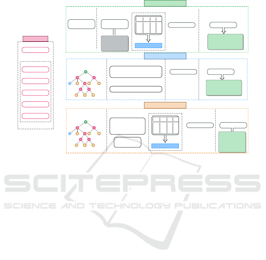
then describes the proposed ITTDTFL model. Fig-

ure 1 depicts the architecture of the ITTFL, DTFL and

ITTDTFL models.

3.1 Background

3.1.1 Fuzzy Logic Model

FL model is based on fuzzy sets where the linguistic

notions and membership functions deﬁne the truth-

value of such linguistic expressions (Zadeh, 1965). A

fuzzy set A in a universe of discourse X is charac-

terized by a membership function µ

(x) that assigns a

value in the interval [0, 1] to each element x in X. This

membership function represents the degree to which

x belongs to the set A. The FL System consists of

four steps (Hentout et al., 2023): Fuzziﬁcation, Fuzzy

knowledge base, Inference engine, and Defuzziﬁca-

tion.

1. Fuzziﬁcation: Consisting of converting numeri-

cal inputs into linguistic variables represented by

membership degrees in fuzzy sets.

2. Fuzzy Knowledge Base: Representing the rela-

tionship between the input variables x and the out-

put variables y. A fuzzy rule has the following

form: ”IF antecedent THEN consequent,” where

both the antecedent and consequent involve lin-

guistic variables and fuzzy sets.

3. Inference Engine: Performing logical deductions

and drawing conclusions based on the rules and

knowledge contained in the system’s knowledge

base.

4. Defuzziﬁcation: Aggregating fuzzy output,

which represents the system’s conclusion or de-

cision, is converted into a crisp that can be easily

understood.

3.1.2 C4.5 Algorithm

C4.5 Algorithm is a DT algorithm developed by Ross

Quinlan (Quinlan, 2014). It is an extension of the ID3

(Iterative Dichotomiser 3). The C4.5 algorithm con-

structs a DT from a given dataset by partitioning data

recursively based on feature attributes. It can handle

ICAART 2024 - 16th International Conference on Agents and Artiﬁcial Intelligence

314

Data

Labeled data

Attribute : A

...

Attribute : A

Class : C

INPUT DATA

Data Pre-

processing

Layer 1

Input Mem-

bership

• Triangular

• Trapezoidal

• Gaussian

Layer 2

... C

T T ... 1

T F ... 1

F T ... 0

Layer 3

Optimized Rules

Defuzziﬁer

Layer 4

Crisp Output

• Degree of mem-

bership to each

class

Layer 5

(a) ITTFL

Layer 1

Membership (Trape-

zoidal) Generation

Fuzzy Rules Generation

Layer 2

Defuzziﬁer

Layer 3

Crisp Output

Layer 4

• Degree of mem-

bership to each

class

(b) DTFL

Layer 1

Membership

Generation

(Trapezoidal)

Fuzzy Rules

Generation

Layer 2

... C

T T ... 1

T F ... 1

F T ... 0

Layer 3

Optimized Rules

Defuzziﬁer

Layer 4

Crisp Output

Layer 5

• Degree of

member-

ship to

each class

Figure 1: The framework of the three models.

numerical and categorical features and is mainly used

for classiﬁcation tasks. The C4.5 algorithm based on

entropy and the information gain allows the genera-

tion of a DT. The equation (1) presents the entropy to

measure the purity and homogeneity within the data

while equation (2) corresponds to information gain to

determine the best attribute to use for data splitting at

each node (Hssina et al., 2014).

Entropy(S) = −

∑

i=1

× log (p

) (1)

Gain(S, T) = Entropy(S) −

∑

j=1

× Entropy(p

))

(2)

Where:

• Entropy(S): The entropy of the dataset S.

• p

: The proportion of instances in S that belong to

class i.

• Gain(S,T ): The gain achieved by splitting the

dataset S using attribute T.

• p

: The set of all possible values for attribute T.

Here is a brief overview of the C4.5 algorithm

steps:

1. The algorithm selects the best attribute for split-

ting the data starting with the root node. The

splitting criterion in C4.5 is based on the entropy

and the information gain ratio, which considers

the number of choices in a given attribute.

2. The algorithm divides the data according to the

selected attribute and then creates child nodes for

each possible attribute value.

3. The algorithm recursively repeats steps 1 and 2 for

each child node until a stopping condition is satis-

ﬁed. This condition may be reaching a maximum

depth, having a minimum number of samples at a

node, or meeting other predeﬁned criteria.

4. The algorithm assigns a class label to each leaf

node based on the dominant class of the training

samples at that node.

5. The algorithm prunes the tree to reduce overﬁtting

by deleting nodes or merging branches.

3.2 Description of the Proposed Model:

ITTDTFL

The ITTDTFL model is an FL-based one that exploits

the knowledge extracted from the C4.5 DT without a

pruning process to provide all the possible and accu-

rate rules and membership functions for the inference

engine. The model’s strength relies on using the TT

technique to optimize the fuzzy rules and membership

functions by merging inclusions of attributes’ inter-

vals that build these rules and membership functions.

Optimization of Fuzzy Rule Induction Based on Decision Tree and Truth Table: A Case Study of Multi-Class Fault Diagnosis

315

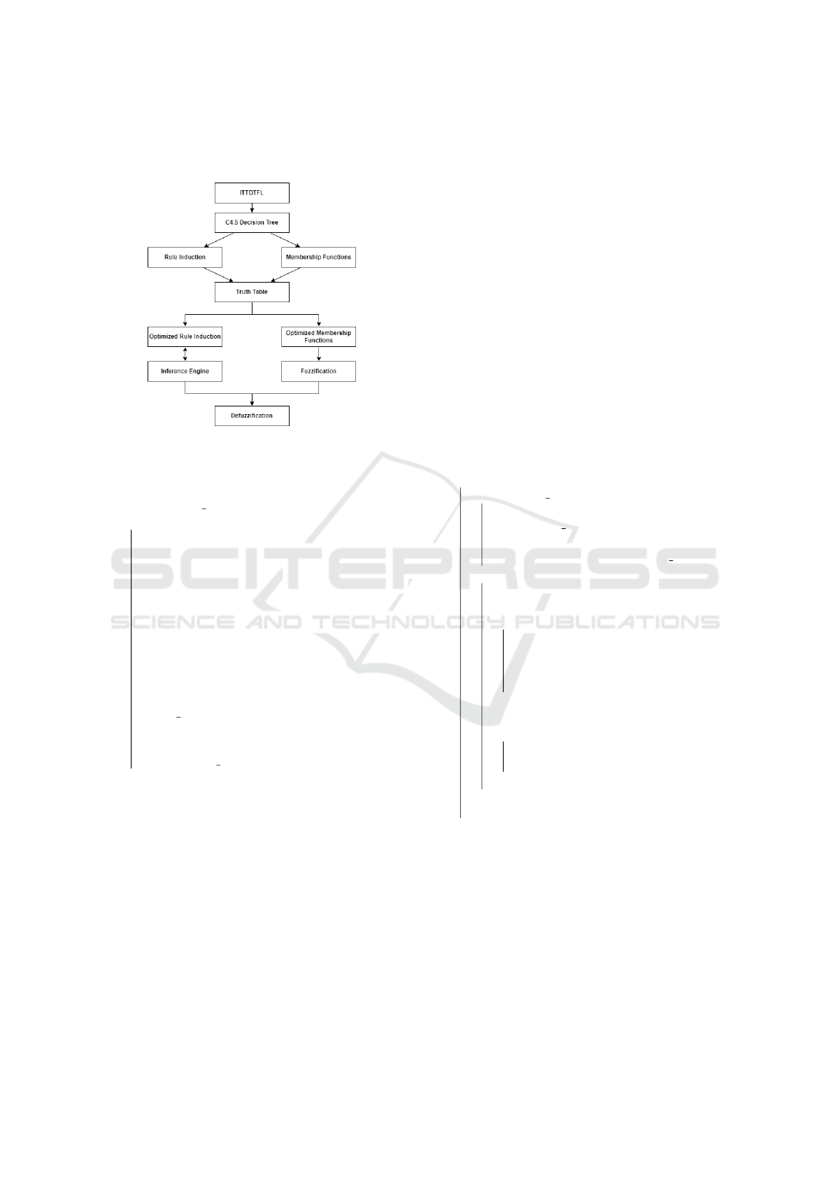
Figure 2 represents the steps of the ITTDTFL model,

whereas the pseudo-code is described in Algorithm 1.

Figure 2: ITTDTFL model ﬂow chart.

Data: dataset D

Result: degree of membership to each class:

Class degree

begin

D ← Read Data;

Tree ← decisionTreeC4.5(D, Features,

Target);

TreeRules ← ruleExtraction(Tree, rules,

currentRule);

Intervals ←

intervalRuleExtraction(TreeRules, Lists);

OIntervals, FuzzyRules ←

truthTable(Intervals, Lists);

MembershipFunctions ← (TrapezoidalMF,

OIntervals);

Class degree ←

fuzzuLogicModel(MembershipFunctions,

FuzzyRules);

return Class degree

end

Algorithm 1: ITTDTFL model.

The algorithm starts by generating a DT

without pruning process from the dataset

using decisionTreeC4.5 function. Next,

ruleExtraction function uses Depth-ﬁrst search

(DFS) to traverse the generated tree from the root

node to the deepest leaves, identifying rules along

each path (see the description in Algorithm 2). For

instance, the output of this step on classifying two

attributes (A

and A

), based on one target (C

), is a

set of rules described in Table 1.

The intervals are then extracted using

intervalRuleExtraction function, where each

line is transformed into a rule containing intervals

of attributes and the corresponding class. Respect-

ing greater than and smaller than symbols (see

Algorithm 3). For example, considering in line 1:

’if (A

<= 0.05) and (A

> 0.015) then class: C

(proba: 100.0%) — based on x samples’, the condi-

tion: (A

<= 0.05) can be written as A

= [X, 0.05],

while the condition: (A

> 0.015) can be written as

= [0.015, Y], where X, Y represents the Min and

Max values that attribute A

, A

can take based on

the dataset. Considering a second line, the condition

is as follows: (A

> 0.05) and (A

<= 0.002) and

> 0) and (A

> 0.001)..., besides A

, attribute A

also can be transformed to an interval; A

= [0.001,

0.002], and so on.

Data: Tree

Result: TreeRules

Function TraverseDecisionTree(node, rules,

currentRule) ;

begin

if node.class label is not Null then

currentRule.append(”class: ” +

node.class label) ;

rules.append(”if ” + currentRule.join(”

and ”) + ” then ” + node.class label) ;

else

if node.attribute is not Null and

node.operator is not Null and

node.threshold is not Null then

currentRule.append(”(” +

node.attribute + ” ” +

node.operator + ” ” +

node.threshold + ”)”) ;

end

for value, childNode in

node.children.items() do

TraverseDecisionTree(childNode,

rules, copy(currentRule)) ;

end

return rules

end

Algorithm 2: ruleExtraction.

This step allows the conversion of every line to

a new rule line containing intervals for each attribute

and its corresponding class, written as: AttributeX

AttributeY

then Class : C

. Next, from these lines,

truthTable function, described in Algorithm 4, is

used to create a TT for interval processing. DTs can

generate a large number of rules and intervals, and

this number is likely to grow as the size and complex-

ICAART 2024 - 16th International Conference on Agents and Artiﬁcial Intelligence

316

Table 1: Example of the output of ruleExtraction function. A represents the attributes, t is the threshold determined from

the tree for each split t ∈ R

if (A

<= t) and (A

<= t) then class: C

(proba: 100.0%) — based on x samples

if (A

> t) and (A

<= t) and (A

> t) and (A

> t) then class: C

(proba: 100.0%) — based on x samples

if (A

> t) and (A

> t) and.... and (A

> t) then class: C

(proba: 100.0%) — based on x samples

...

Data: TreeRules

Result: Intervals

begin

Initialize intervals dictionary {A

: [ ], A

[ ]};

Deﬁne patterns: Interval patterns (”A

≤

value”, ”A

> value”), Class pattern

(”Class : value”);

foreach line in TreeRules do

foreach match in line using patterns do

Extract attribute (A

or A

) and

value;

Convert value to a ﬂoating-point

number;

Update intervals[A

] or

intervals[A

] with the extracted

value;

Extract the Class and the value;

Convert the value to string;

Update Class with the extracted

value;

end

index = [start, end] & A

index =

[start, end] Class : C

;

save to Intervals;

end

Algorithm 3: intervalRuleExtraction.

ity of the data increases. Therefore, these intervals

must pass through the proposed process in order to

be reduced to avoid useless computations. The TT

approach identiﬁes and merges the inclusions within

the extracted intervals. The TT contains attributes,

for example, two attributes A

, A

, and the classes as

columns, while in rows, there are intervals I

and I

for each state, 1 if the class is true 0 if it is false, as

shown in Table 7. First, a grouping process of the

attributes by class (where Class = 1), then for each

group, it compares the extracted intervals for each at-

tribute. Technically, it creates a list for each row of

attributes in the group L

& L

of intervals. Next, a

comparison between intervals of each list is made. A

merging process of the inclusions is executed. Taking

for example L

contains 4 sets or intervals I

, I

and I

as Figure 3 shows, it is obvious that inter-

val I

includes I

and I

includes I

, thus, only

and I

will be kept and respectively replace in-

tervals I

and I

. The use of such an approach has

notably reduced the number of intervals as well as the

extracted rules.

Figure 3: L

Intervals inclusion property.

After having the TT’s ﬁnal version, all the inter-

vals left are transformed into Trapezoidal Member-

ship Functions using membershipF function. The

trapezoidal membership function is a graph represent-

ing the degree to which an element belongs to a cer-

tain fuzzy set. It has four parameters: the left and

right edges, a lower plateau, and an upper plateau.

These parameters determine the shape of the trape-

zoid, which represents the fuzzy sets. For example, a

fuzzy set of ”tall people.” the trapezoidal membership

function for this set could have the following param-

eters:

• Left boundary point: 150 cm

• Right boundary point: 200 cm

• Lower plateau: 160 cm

• Upper plateau: 190 cm

We chose this type of membership function based

on previous work comparing the Trapezoidal mem-

bership function with Triangular and Gaussian mem-

bership function (Kerarmi et al., 2022). Based on the

results, adopting the Trapezoidal membership func-

tion for an FL model gave better results simply be-

cause it rates the degree of belonging at 100% that

an element belongs to a fuzzy anywhere between the

lower and upper plateau. For example, if we use ’Tall’

as a linguistic term to describe values that fall within

the upper and lower plateaus, it means all people be-

tween 160 and 19 cm are Tall. Unlike the Triangu-

Optimization of Fuzzy Rule Induction Based on Decision Tree and Truth Table: A Case Study of Multi-Class Fault Diagnosis

317

Data: Intervals

Result: OIntervals

Initialize an empty truth table, a 2D array with

rows for each data point and columns for each

class;

while Reading lines do

foreach each line in the lines do

Initialize an empty row in the truth

table with all zeros;

Extract the values of attribute 1 and

attribute 2 from the current line;

foreach each class do

if attribute 1 is in the class’s

interval AND attribute 2 is in the

class’s interval then

Set the corresponding cell in

the truth table to 1;

end

Group table by Class = 1;

Initialize an empty list S for storing

optimized intervals;

S ← Group;

← length(I

);

← length(I

);

foreach two intervals I

and I

in S do

if I

[1] ≤ I

[1] AND I

] ≥ I

] then

S ← S \ {I

}

end

Algorithm 4: truthTable.

lar and Gaussian membership functions, an element

100% belongs to a fuzzy set only if it is equal to the

median of the fuzzy set. Since the vagueness is also

represented in the uncertain belonging degree of an

element to a particular fuzzy set, logically, the Trape-

zoidal membership function is the best.

Rules are extracted from the table, where each

row represents a rule. Noting that during the extrac-

tion of the rules, we considered extracting these rules

in a required format to go straight to the rule base:

rule

= ctrl.Rule(Attribute

[’MembershipFunction

’]

&Attribute

p+1

[’MembershipFunction

’],Class[’C

’]).

Finally, all the requirements of an FL model are

satisﬁed, and Fuzzy sets and fuzzy rules are automat-

ically generated and well-optimized. The function

fuzzuLogicMode is used to build an FL model, the

ﬁnal step in our model.

The model identiﬁes the logic between data, ex-

tracts, describes, and represents the knowledge from

this data. This part is described in the Experiments

Section. For the sake of simplicity, the models return

the set of failure classes with their probabilities. This

probability can be seen as a measure of the likelihood

of an occurrence of a failure in real-time. Table 2 rep-

resents an extract of rules from the DT.

Table 2: Short example of extracted rules from the DT.

rule1 = ctrl.Rule(A

value[’A

’], Class[’C

’])

rule2 = ctrl.Rule(A

value[’A

’] & A

value[’A

’], Class[’C

’])

rule3 = ctrl.Rule(A

value[’A

’] & A

value[’A

’], Class[’C

’])

...

4 EXPERIMENTS & RESULTS

In order to evaluate our model performance, we

benchmark the algorithms DTFL and ITTDTFL with

C4.5, FURIA, and Ripper from WEKA library (Wit-

ten et al., 2005) implemented using Python 3.8 in

the same environment. The evaluation is done by

conducting a series of experiments based on several

factors (Hambali et al., 2019), including the number

of generated rules, computational time, accuracy in

Equation 3, and other metrics such as F1-score which

indicates the model’s capabilities of avoiding false

positives (recall) while identifying positive examples

(precision) in Equation 6, Sensitivity/recall which

evaluates the model’s predictions of true positives of

each available category in Equation 7, and Receiver

Operating Characteristic Curve (ROC) area which in-

dicates the model performance at distinguishing be-

tween the classes. The performance of the ﬁve models

is extensively demonstrated using three sets of data

related to pump failure instances. The description of

the data, the experiment protocol, and the obtained

results are demonstrated later in this section.

Accuracy =

TP + TN

TP + FP + TN + FN

(3)

Precision =

TP + FP

(4)

Recall =

TP + FN

(5)

F-Measure =

2(Precision-Recall)

(Precision + Recall)

(6)

where TP is the True Positive, TN is the True Neg-

ative, FP is the False Positive ad FN is the False Neg-

ative.

ICAART 2024 - 16th International Conference on Agents and Artiﬁcial Intelligence

318

4.1 Datasets

Two real datasets were collected from two pumps.

The data captures various operational parameters,

such as the acceleration time waveform (g), velocity

spectrum ( f f tv), and acceleration spectrum ( f f tg),

saved as lists of observations, as well as the failure

class based on the results of a regularly performed

Failure Mode and Effect Critical Analysis method

(FMECA) (Kerarmi et al., 2022). It contains seven

classes where one is a normal state, and six others cor-

respond to different failures. All the datasets include

measurements from several sensors installed through-

out the machine. Table 3 represents a statistical data

view, while Table 4 describes their form. The third

dataset is the combination of the two datasets. These

rich and comprehensive datasets provide a detailed

view of system behavior and form the basis for perfor-

mance analysis and classiﬁcation of potential failures.

Additionally, these datasets have been pre-processed

to eliminate outliers and missing values before further

analysis.

Table 3: Datasets statistical description.

Dataset Number of rows

1 4016

2 3048

3 7064

Table 4: Datasets description.

fftv

fftg

MSC

P1- P2- P3- P4

Numerical data

Normal State

Imbalance

Structural fault

Misalignment

Mechanical looseness

Bearing lubrication

Gear fault

Sensor position;

Acceleration time waveform;

Velocity spectrum;

Acceleration spectrum;

Machine State Class.

First, We calculate the Root Mean Square (RMS)

values of ( f f tv) and ( f f tg) since they are critical fac-

tors for machinery status diagnosis for signal normal-

ization and to reduce variability. Equation (7) depicts

the formula based on this study (Rzeszucinski et al.,

2012). We calculate the RMS of all the lists in f f tv

and f f tg of each machine state class identiﬁed by the

FMECA method using the following formula:

rms



+ x

+ ··· + x



(7)

We ﬁnally got rows that include the root mean

square (RMS) values of f f tv and f f tg for the seven

described machine state classes, this provides essen-

tial information for the modeling, training, and test-

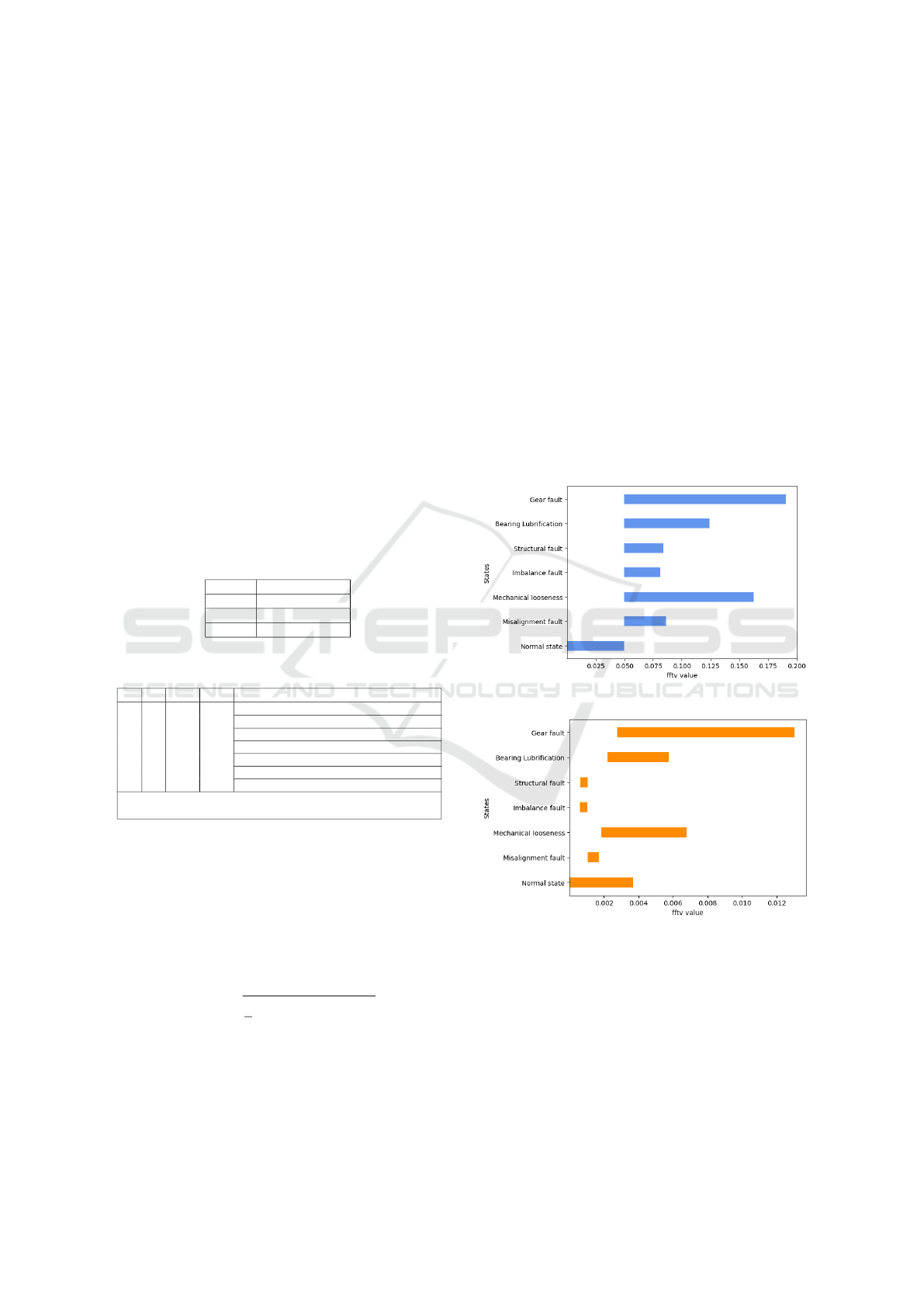
ing of the proposed models. Figures 4 and 5 represent

the values of f f tv and f f tg plotted as intervals. The

deﬁnition of speciﬁc values of each state is compli-

cated and challenging, given the inclusions and inter-

sections between intervals, as Figures 4 and 5 show.

Therefore, we employed the C4.5 algorithm to ex-

tract knowledge from the dataset, this knowledge is

represented as rules that determine the path from the

root node to a child node containing the class name,

with these paths being based on the attributes f f tv

and f f tg. Table 5 represents the extracted knowl-

edge from the generated DT. Based on the DT results,

each row contains thresholds that are used to create

intervals f f tv

and f f tg

of each attribute f f tv and

f f tg for each class C. This knowledge is represented

by intervals for classes and converted into a Trape-

zoidal membership function and Fuzzy rules for the

FL model. Table 6 shows an extract of rules from the

DT.

Figure 4: f f tv values for each state.

Figure 5: f f tg values for each state.

The TT is used directly to merge intervals and

avoid rule redundancy, thus considerably reducing the

number of rules and membership functions. This has

proved effective in the computational time taken for

the model ITTDTFL. Table 7 represents the generated

TT used for the inclusion merging process.

In the merging process as described in the

Methodology Section, the model groups the rows by

class where this latter is true equals 1. Then, for each

Optimization of Fuzzy Rule Induction Based on Decision Tree and Truth Table: A Case Study of Multi-Class Fault Diagnosis

319

Table 5: An extract of the knowledge using the DT.

if (fftv <= 0.05) then class: Normal state (proba: 100.0%) — based on 1,513 samples

if (fftv <= 0.05) and (fftg <= 0.002) and (fftg <= 0.001) then class: Misalignment fault (proba: 100.0%) — based on 241 samples

if (fftv <= 0.05) and (fftg <= 0.002) and (fftg <= 0.007) and (fftv <= 0.075) and (fftv <= 0.099) and (fftg <= 0.005) then class: Mechanical looseness fault (proba: 100.0%) — based on 32 samples

if (fftv > 0.05) and (fftg <= 0.002) and (fftg <= 0.001) and (fftv <= 0.073) and (fftv <= 0.081) then class: Structural fault (proba: 100.0%) — based on 8 samples

if (fftv > 0.05) and (fftg <= 0.002) and (fftg <= 0.007) and (fftg <= 0.007) then class: Gear fault (proba: 100.0%) — based on 8 samples

if (fftv > 0.05) and (fftg <= 0.002) and (fftg <= 0.007) and (fftg <= 0.007) and (fftg <= 0.007) then class: Gear fault (proba: 100.0%) — based on 1 samples

if (fftv > 0.05) and (fftg <= 0.002) and (fftg <= 0.007) and (fftv <= 0.075) and (fftg <= 0.003) and (fftv <= 0.05) then class: Gear fault (proba: 100.0%) — based on 1 samples

if (fftv > 0.05) and (fftg <= 0.002) and (fftg <= 0.007) and (fftg <= 0.007) and (fftg <= 0.007) then class: Mechanical looseness fault (proba: 100.0%) — based on 1 samples

...

Table 6: Short example of extracted rules from the DT.

rule1= ctrl.Rule( f f tv[’ f f tv

’], Class[’Normal state’])

rule2= ctrl.Rule( f f tv[’ f f tv

’] & f f tg[’ f f tg

’], Class[’Misalignment fault’])

rule3= ctrl.Rule( f f tv[’ f f tv

’] & f f tg[’ f f tg

’], Class[’Mechanical looseness fault’])

rule4= ctrl.Rule( f f tv[’ f f tv

’] & f f tg[’ f f tg

’], Class[’Imbalance fault’])

rule5= ctrl.Rule( f f tv[’ f f tv

’] & f f tg[’ f f tg

’], Class[’Imbalance fault’])

rule6= ctrl.Rule( f f tv[’ f f tv

’] & f f tg[’ f f tg

’], Class[’Structural fault’])

rule7= ctrl.Rule( f f tv[’ f f tv

’] & f f tg[’ f f tg

’], Class[’Mechanical looseness fault’])

rule8= ctrl.Rule( f f tv[’ f f tv

’] & f f tg[’ f f tg

’], Class[’Mechanical looseness fault’])

rule9= ctrl.Rule( f f tv[’ f f tv

’] & f f tg[’ f f tg

’], Class[’Structural fault’])

rule10= ctrl.Rule( f f tv[’ f f tv

’] & f f tg[’ f f tg

’], Class[’Mechanical looseness fault’])

Table 7: TT used for the inclusion merging process.

fftv fftg Bearing Lubrication fault Gear fault Imbalance fault Mechanical looseness fault Misalignment fault Normal state Structural fault

f f t v

None 0 0 0 0 0 1 0

f f t v

f f t g

0 0 0 0 1 0 0

f f t v

f f t g

0 0 0 1 0 0 0

f f t v

f f t g

0 0 1 0 0 0 0

f f t v

f f t g

0 0 1 0 0 0 0

column of the attributes f f tv and f f tg, each interval

is compared to other intervals to check for inclusion;

if any inclusion was found, the major interval takes

place in the included interval, and so on. These in-

tervals are converted to membership functions, Fig-

ure 6 represents membership functions of dataset 3

before optimization. Note that the number of gener-

ated membership functions is 130 for fftv and 17 for

f f tg. Algorithm 4 has signiﬁcantly reduced the num-

ber of membership functions, avoiding useless com-

putational effort. The outputs of the optimized mem-

bership functions are represented in Figure 7. Finally,

by eliminating the redundancies, the TT contains a

signiﬁcantly reduced number of rules and the inter-

vals used for creating membership functions.

4.2 Experiment Protocol

We conducted a series of experiments and split the

datasets into training (75%) and testing sets (25%).

Table 8 depicts the number of samples used in the

training and testing phases and the total number of

samples of each dataset.

Table 8: Training/Testing samples.

Dataset Total number Training set Testing set

1 4016 3009 1007

2 3048 2284 764

3 7064 5295 1769

4.3 Results & Discussion

Table 9 shows the performances in terms of the num-

ber of generated membership functions for FL-based

models, notably DTFL and ITTDTFL models. Ta-

ble 10 represents the number of generated rules and

the computational time of all models, while Table 11

depicts the classiﬁcation metrics, including the accu-

racy, sensitivity, F1-score, and ROC area scores.

Table 9: Number of generated Membership Functions.

Model Dataset

Generated Membership Functions number

fftv

fftg

DTFL

1 110 19

2 57 13

3 130 17

ITTDTFL

1 20 7

2 5 10

3 10 7

Regarding computational time and rule number, the

FURIA algorithm took 28.73, 8.74, and 45.6 seconds

for each dataset to be classiﬁed, generating 30, 22,

and 31 rules, respectively. RIPPER consistently re-

quired longer computational time, from 302.54 sec-

onds to 1277.68 seconds, generating 17, 14, and 20

rules in each experiment. As it is noticed, although

the number of rules is relatively small, it took a sig-

niﬁcant amount of time in order to give results, sim-

ply because they need to search for all possible rules

that can be used for data classiﬁcation, as the dataset

size increases, it is expected that a model’s computa-

tional time requirements also proportionally increase.

Apparently, RIPPER’s requirements have exponen-

ICAART 2024 - 16th International Conference on Agents and Artiﬁcial Intelligence

320

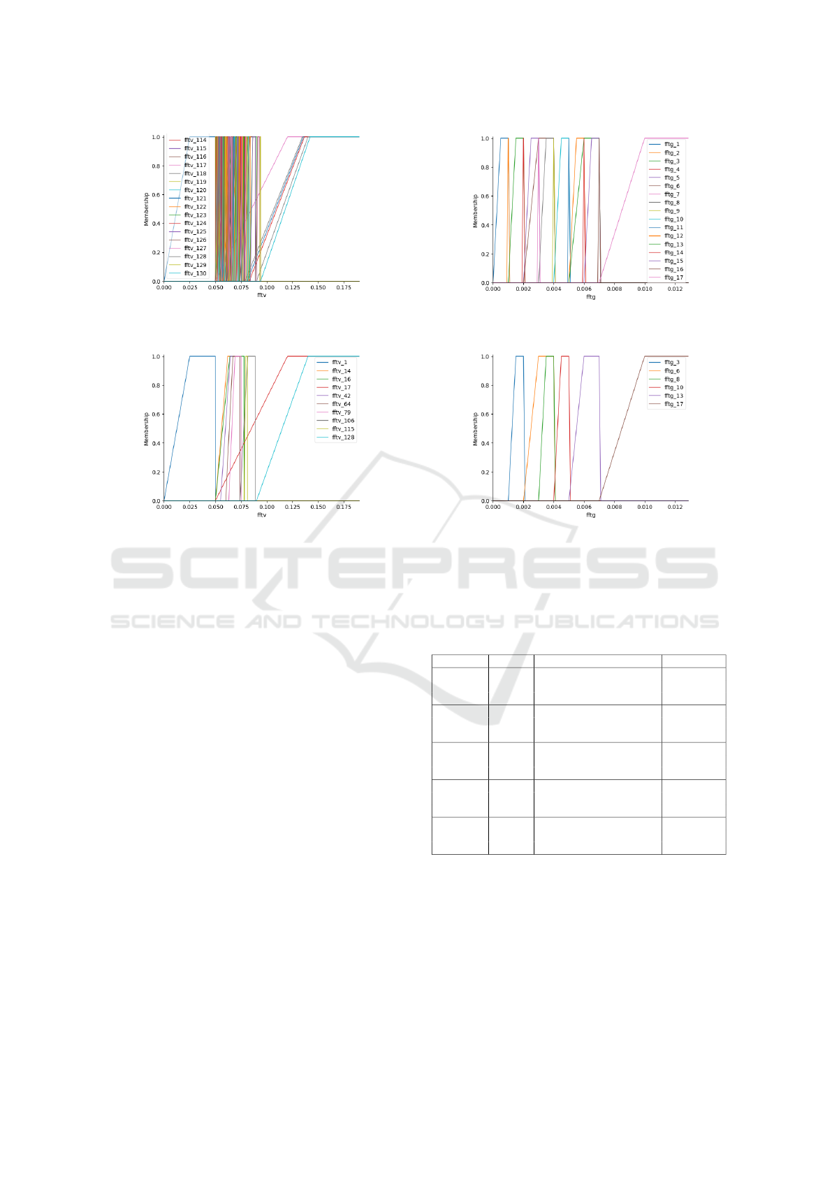
(a) fftv Membership Function

(b) fftg Membership Function

Figure 6: Membership Functions.

(a) fftv Membership Function (b) fftg Membership Function

Figure 7: Optimized Membership Functions.

tially increased. However, the C4.5 algorithm was

the fastest, with 1.2 seconds on average, due to the

gain ratio method used for splitting the data, which

considers the information gain and the number of val-

ues in an attribute. This helps reduce the number of

splits required to build the decision tree, making the

algorithm faster. In terms of rules, the C4.5 algorithm

has generated 23, 10, and 15 rules with the pruning

process. However, it fell short of the desired perfor-

mance levels in terms of classiﬁcation accuracy. For

FL-based models, DTFL also took an important com-

putational time due to the number of generated rules,

in the worst case, 287 rules in 364.38 s. Therefore,

it is crucial to reduce the number of rules in order

to build a faster model. Meanwhile, ITTDTFL has

achieved a signiﬁcant reduction rate of the rules by

approximately 86.87%, from 202 to 28 on dataset 1,

89 to 15 on dataset 2, and 287 to 24 on dataset 3.

Moreover, the number of the generated membership

functions is also notably optimized compared to the

DTFL model, as shown in Table 10, ITTDTFL model

successively reduced the number of generated mem-

bership functions fftv/fftg, from 110/19 to 20/7, 57/13

to 5/10, and 130/17 to 10/7 withing the three datasets.

To better represent the differences between models

and the critical impact of the number of rules on the

computational time, Figure 8 projects the number of

rules on the total time taken by the model in the three

tests.

Table 10: Number of rules and computational time of each

model.

Model Dataset Number of generated rules Runtime (s)

FURIA

1 30 28.73

2 22 8.74

3 31 45.62

RIPPER

1 17 674.24

2 14 302.54

3 20 1277.68

C4.5

1 23 1.51

2 10 0.43

3 15 1.79

DTFL

1 202 127.82

2 89 23.65

3 287 364.38

ITTDTFL

1 28 7.45

2 15 3.1

3 24 16.08

Optimization of Fuzzy Rule Induction Based on Decision Tree and Truth Table: A Case Study of Multi-Class Fault Diagnosis

321

Figure 8: Runtime vs rules number plot.

Table 11: Classiﬁcation performance of each model.

Model Dataset Accuracy (%) Sensitivity F1-Score ROC

FURIA

1 90.28% 0.90 0.90 0.97

2 93.56% 0.93 0.93 0.98

3 91.59% 0.91 0.91 0.97

RIPPER

1 88.14% 0.88 0.88 0.98

2 93.08% 0.93 0.93 0.99

3 91.14% 0.91 0.91 0.99

C4.5

1 88.54% 0.88 0.88 0.98

2 92.78% 0.92 0.92 0.99

3 90.48% 0.90 0.90 0.99

DTFL

1 91.45% 0.91 0.90 0.87

2 95.41% 0.95 0.94 0.92

3 93.15% 0.93 0.93 0.89

ITTDTFL

1 97.91% 0.97 0.97 0.95

2 95.94% 0.95 0.95 0.90

3 98.92% 0.98 0.98 0.95

In terms of accuracy, the results obtained from

the experiments show that all models did a good job

classifying the machine state classes. Considering

the number of correct classiﬁcations, all models have

achieved high accuracy rates, with only a few misclas-

siﬁcations. FURIA, RIPPER, and C4.5 have shown

good performances during the different experiments.

As expected from these evaluations and others in the

literature, FURIA gave the best results, correctly clas-

sifying data ranging from 90.28% to 93.56%, for FU-

RIA, 88.14% to 93.08% for RIPPER, while C4.5 cor-

rectly classiﬁed 88.54% to 92.78%. For FL-based

models, the DTFL model also gave good results in

terms of accuracy, ranging from 91.45% to 93.49%.

Meanwhile, ITTDTFL exhibited excellent accuracies

for the three data sets, it attended 95.94%, 97.91%,

and 98.92%, accurately classifying the data, enhanc-

ing the DTFL model’s accuracy by 4.55% and out-

performed FURIA, RIPPER, C4.5 successively by

6.92%, 7.5%, 7.32%. These results can be explained

by the fact that TT can preserve the most accurate

and meaningful membership function corresponding

to each class, improving the precision of each fuzzy

rule and leading to better classiﬁcation accuracy. In

terms of other metrics, as shown in Table 11, consid-

ering 0.9-1.0 is Excellent, and 0.8-0.9 is Good, all the

models achieved good to excellent scores in ROC area

metric, as well as for sensitivity and F1-score metrics.

To sum up, ITTDTFL successfully optimizes the

number of membership functions and accurately in-

ducts rules for the FL model. DT is used to generate

intervals and rules from the paths of each branch. At

the same time, TT eliminates inclusions within gen-

erated intervals from these paths, addressing the is-

sue of duplicated sub-trees and enhancing feature cap-

ture. This approach results in signiﬁcantly reduced

computational time and improved classiﬁcation per-

formance. Compared to the related work’s results,

the ITTDTFL model has signiﬁcantly outperformed

FURIA, RIPPER, C4.5 algorithm, and DTFL model

by 4.55% to 7.5% in terms of accuracy and computa-

tional time. The ITTDTFL model is very interpretable

and easy to manipulate due to its simple structure, do-

main expert involvement, transparent algorithms, and

Human-Understandable rules.

5 CONCLUSIONS & FUTURE

WORKS

This paper proposes a fusion between TT, FL, and

DT to generate optimized membership functions and

rules for FL. This combination shows promising re-

sults for the multi-classiﬁcations domain. The TT is

the key in the ITTDTFL model, it generates accu-

rate and optimized membership functions and rules.

The ITTDTFL model has successfully outperformed

the most known multi-classiﬁcation models, such as

FURIA, RIPPER, C4.5, and DTFL. A notable advan-

tage of integrating the TT into this process is the sig-

niﬁcant rule number reduction by 86.87%. This fu-

sion played a signiﬁcant role in improving the op-

timized rules’ generation and enhancing their preci-

sion. Which in turn leads to achieving impeccable

accuracies in data classiﬁcation as well as in compu-

tational time. ITTDTFL has successfully reduced the

computational time for the DTFL model by 92.87%,

enhancing its accuracy by 4.55%. At the same time,

passing the other models, FURIA, RIPPER, and C4.5,

successively by 6.92%, 7.5%, and 7.32%. Real ma-

chine fault datasets were used for the evaluation. It

has seven classes and Two complicated attributes (ve-

locity and acceleration spectrums), noting that hav-

ing more attributes would enhance the precision of

the rules and, consequently, the model. This model

offers promising potential for delivering accurate re-

sults in real-time. Demonstrating its versatility, this

model is highly interpretable and can be applied to

various classiﬁcation issues beyond machine condi-

tion diagnosis. Thus, the next step is to apply this

model to the datasets used in the literature, such as

UCI and Statlib repositories, as well as investigate

the integration of multi-objective optimization using

Evolutionary algorithms, such as genetic algorithms,

ICAART 2024 - 16th International Conference on Agents and Artiﬁcial Intelligence

322

which will certainly enhance the model’s capabilities

of accurately classifying the data as well as its com-

putational time requirements.

REFERENCES

Al-Shammaa, M. and Abbod, M. F. (2014). Automatic

generation of fuzzy classiﬁcation rules from data. In

Proc. of the 2014 International Conference on Neural

Networks-Fuzzy Systems (NN-FS 14), Venice.

Angelov, P. P. and Buswell, R. A. (2003). Automatic gener-

ation of fuzzy rule-based models from data by genetic

algorithms. Information Sciences, 150(1-2):17–31.

Bertsimas, D. and Dunn, J. (2017). Optimal classiﬁcation

trees. Machine Learning, 106:1039–1082.

Chi, Z., Yan, H., and Pham, T. (1996). Fuzzy algorithms:

with applications to image processing and pattern

recognition, volume 10. World Scientiﬁc.

Chiu, S. (1997). Extracting fuzzy rules from data for func-

tion approximation and pattern classiﬁcation.

Cintra, M. E., Monard, M. C., and Camargo, H. A. (2013).

A fuzzy decision tree algorithm based on c4. 5. Math-

ware & Soft Computing, 20(1):56–62.

Cohen, W. W. (1995). Fast effective rule induction. In Ma-

chine learning proceedings 1995, pages 115–123. El-

sevier.

Durkin, J. (1990). Research review: Application of expert

systems in the sciences. The Ohio Journal of Science,

90(5):171–179.

Elbaz, K., Shen, S.-L., Zhou, A., Yuan, D.-J., and Xu, Y.-S.

(2019). Optimization of epb shield performance with

adaptive neuro-fuzzy inference system and genetic al-

gorithm. Applied Sciences, 9(4):780.

omez-Skarmeta, A. F., Delgado, M., and Vila, M. A.

(1999). About the use of fuzzy clustering techniques

for fuzzy model identiﬁcation. Fuzzy sets and systems,

106(2):179–188.

Gonzblez, A. and P

erez, R. (1999). Slave: A genetic learn-

ing system based on an iterative approach. IEEE

Transactions on fuzzy systems, 7(2):176–191.

Hambali, A., Yakub, K., Oladele, T. O., and Gbolagade,

M. D. (2019). Adaboost ensemble algorithms for

breast cancer classiﬁcation. Journal of Advances in

Computer Research, 10(2):31–52.

Hentout, A., Maoudj, A., and Aouache, M. (2023). A re-

view of the literature on fuzzy-logic approaches for

collision-free path planning of manipulator robots. Ar-

tiﬁcial Intelligence Review, 56(4):3369–3444.

Hssina, B., Merbouha, A., Ezzikouri, H., and Erritali, M.

(2014). A comparative study of decision tree id3 and

c4. 5. International Journal of Advanced Computer

Science and Applications, 4(2):13–19.

uhn, J. and H

ullermeier, E. (2009). Furia: an algorithm

for unordered fuzzy rule induction. Data Mining and

Knowledge Discovery, 19:293–319.

uhn, J. C. and H

ullermeier, E. (2010). An analysis of

the furia algorithm for fuzzy rule induction. In Ad-

vances in Machine Learning I: Dedicated to the Mem-

ory of Professor Ryszard S. Michalski, pages 321–344.

Springer.

ullermeier, E. (2011). Fuzzy sets in machine learning and

data mining. Applied Soft Computing, 11(2):1493–

1505.

Kerarmi, A., Kamal-idrissi, A., Seghrouchni, A. E. F., et al.

(2022). An optimized fuzzy logic model for proactive

maintenance. In CS & IT Conference Proceedings,

volume 12. CS & IT Conference Proceedings.

Kontogiannis, D., Bargiotas, D., and Daskalopulu, A.

(2021). Fuzzy control system for smart energy man-

agement in residential buildings based on environ-

mental data. Energies, 14(3):752.

Mousavi, S. M., Tavana, M., Alikar, N., and Zandieh, M.

(2019). A tuned hybrid intelligent fruit ﬂy optimiza-

tion algorithm for fuzzy rule generation and classiﬁ-

cation. Neural Computing and Applications, 31:873–

885.

Mutlu, B., Sezer, E. A., and Akcayol, M. A. (2018). Auto-

matic rule generation of fuzzy systems: A compar-

ative assessment on software defect prediction. In

2018 3rd International Conference on Computer Sci-

ence and Engineering (UBMK), pages 209–214.

Prado, R., Garcia-Gal

an, S., Exposito, J. M., and Yuste,

A. J. (2010). Knowledge acquisition in fuzzy-

rule-based systems with particle-swarm optimization.

IEEE Transactions on Fuzzy Systems, 18(6):1083–

1097.

Quinlan, J. R. (2014). C4. 5: programs for machine learn-

ing. Elsevier.

Reddy, G. T., Reddy, M. P. K., Lakshmanna, K., Rajput,

D. S., Kaluri, R., and Srivastava, G. (2020). Hybrid

genetic algorithm and a fuzzy logic classiﬁer for heart

disease diagnosis. Evolutionary Intelligence, 13:185–

196.

Ren, Q., zhang, H., Zhang, D., Zhao, X., Yan, L., and Rui,

J. (2022). A novel hybrid method of lithology identi-

ﬁcation based on k-means++ algorithm and fuzzy de-

cision tree. Journal of Petroleum Science and Engi-

neering, 208:109681.

Rzeszucinski, P., Sinha, J. K., Edwards, R., Starr, A., and

Allen, B. (2012). Normalised root mean square and

amplitude of sidebands of vibration response as tools

for gearbox diagnosis. Strain, 48(6):445–452.

Tran, T. T., Nguyen, T. N., Nguyen, T. T., Nguyen, G. L.,

and Truong, C. N. (2022). A fuzzy association rules

mining algorithm with fuzzy partitioning optimization

for intelligent decision systems. International Journal

of Fuzzy Systems, 24(5):2617–2630.

Varshney, A. K. and Torra, V. (2023). Literature review

of the recent trends and applications in various fuzzy

rule-based systems. International Journal of Fuzzy

Systems, pages 1–24.

Witten, I. H., Frank, E., Hall, M. A., Pal, C. J., and Data,

M. (2005). Practical machine learning tools and tech-

niques. In Data mining, volume 2, pages 403–413.

Elsevier Amsterdam, The Netherlands.

Zadeh, L. A. (1965). Fuzzy sets. Information and control,

8(3):338–353.

Optimization of Fuzzy Rule Induction Based on Decision Tree and Truth Table: A Case Study of Multi-Class Fault Diagnosis

323