Scheduling Onboard Tasks of the NIMPH Nanosatellite

Julien Rouzot

1,2

, Jos

ephine Gobert

, Christian Artigues

, Romain Boyer

, Fr

eric Camps

Philippe Garnier

, Emmanuel Hebrard

and Pierre Lopez

LAAS-CNRS, Toulouse, France

IRAP, Toulouse, France

{ﬁrstname.lastname}@laas.fr, {ﬁrstname.lastname}@irap.omp.eu

Keywords:

Scheduling, Constraint Programming, Nanosatellite, Hypervisor.

Abstract:

In the context of terrestrial space missions, thanks to the recent development of micro and nanotechnologies,

nanosatellites are becoming increasingly popular for their lower cost and ease of deployment. The NIMPH

(Nanosatellite to Investigate Microwave Photonics Hardware) mission is an ongoing academic project aimed at

developing and launching such a nanosatellite. The onboard resources on these missions are often very limited,

and in our study case, a single onboard computer is responsible for orchestrating the science and avionic tasks

of the nanosatellite. These tasks are subject to various constraints, such as frequency, minimum/maximum

delay between the execution of the same type of task and strict precedences. This makes the scheduling of

the onboard tasks a challenging problem, which is critical for the mission success. In this paper, we tackle

the problem of scheduling NIMPH onboard tasks using Constraint Programming methods. Our scheduler

demonstrates its performance by generating optimal or near-optimal schedules for the NIMPH nanosatellite.

1 INTRODUCTION

The NIMPH mission is part of the Nanolab-Academy

project proposed by the CNES (French Space

Agency) that encourages students to engage in space

exploration by developing, launching and exploiting

their nanosatellites of type CubeSat, through intern-

ships and academic projects (CNES, 2021). NIMPH

stands for Nanosatellite to Investigate Microwave

Photonics Hardware. This project is still in its de-

velopment phase (C), with a launch planned for 2025.

From a general perspective, the nanosatellite’s mis-

sion is to evaluate the inﬂuence of the space environ-

ment on optoelectronic components (Landrea et al.,

2018).

The nanosatellites developed in the context of

Nanolab-Academy use the same ﬂight software pro-

vided by CNES. The science and avionic opera-

tions are driven by dedicated and isolated parti-

tions (Windsor and Hjortnaes, 2009), that are orches-

trated by the onboard computer (OBC) hypervisor.

ΧTratuM (Masmano et al., 2009) is used to manage

the execution of these partitions. This bare-metal hy-

pervisor is a software developed by the Spanish com-

pany FentISS and has been widely used for space mis-

sions.

The partitions represent the containers of all

the different tasks that must be performed by the

nanosatellite, such as orientation correction, scientiﬁc

measures, uplink command management, and more.

As the OBC is unable to perform any sort of multi-

processing, the partitions must be executed sequen-

tially and cannot overlap. To simplify the scheduling

of the OBC tasks for Nanolab nanosatellite missions,

the team developing the ﬂight software chose to make

the schedule cyclic, with a ﬁnite time horizon of one

second. This means the OBC will repeat the same

partitions executions every cycle. A ﬁxed number of

tasks (i.e., partition execution of constant duration)

for each partition must be performed within this time

horizon. In the context of the NIMPH mission, due to

the number of tasks and the various constraints on the

partitions, obtaining manually the OBC schedule is an

extremely challenging work. Finally, the best sched-

ules aim to maximize the effective use of the schedule

time, which corresponds to the sum of the task dura-

tion minus the number of context switches, that hap-

pen between the execution of two different partitions

and are time-consuming. This aspect makes the cyclic

scheduling of NIMPH tasks even harder.

ΧTratuM comes with ΧoncretE (Balbastre et al.,

2021), a dedicated scheduler that allows the genera-

tion of a cyclic execution plan of the different parti-

tions, that minimizes the number of context switches.

Rouzot, J., Gobert, J., Artigues, C., Boyer, R., Camps, F., Garnier, P., Hebrard, E. and Lopez, P.

Scheduling Onboard Tasks of the NIMPH Nanosatellite.

DOI: 10.5220/0012378500003639

Paper published under CC license (CC BY-NC-ND 4.0)

In Proceedings of the 13th International Conference on Operations Research and Enterprise Systems (ICORES 2024), pages 277-284

ISBN: 978-989-758-681-1; ISSN: 2184-4372

277

This tool has a major drawback: most constraints on

the NIMPH cyclic task scheduling problem cannot be

expressed within ΧoncretE. This makes the genera-

tion of valid schedules a laborious work, as the plans

must be manually reﬁned to match the real constraints

(at least in the context of the NIMPH mission). This

also often leads to poorer solutions.

In this context, we propose NanoSatScheduler

a scheduler based on Constraint Programming meth-

ods, that tackles NIMPH’s speciﬁc constraints, while

being generic enough to handle OBC partition

scheduling for other nanosatellite missions. We ﬁrst

introduce the NIMPH cyclic task scheduling problem

formally and compare it to other similar scheduling

problems in the literature. We then highlight two con-

straint programming models, NanoSat and NanoSat-

Global, using the IBM CP Optimizer solver, to solve

the NIMPH cyclic task scheduling problem. We also

present NanoSatIterative, an iterative method to max-

imize the effective schedule time by adding new tasks

while minimizing the number of context switches and

keeping the optimality proof. These methods are eval-

uated on synthetic instances based on NIMPH param-

eters to demonstrate their performance. We ﬁnally

conclude on the limitations and future work for our

scheduler.

2 THE NIMPH CYCLIC TASK

SCHEDULING PROBLEM

2.1 Formal Description

To handle the scientiﬁc and avionic tasks of the

NIMPH nanosatellite, the main software is divided

into a ﬁnite set of N partitions, denoted P =

, P

, . . . , P

}. We can refer to a particular parti-

tion by its name (e.g., P

IOS

for IOS partition). These

partitions can be seen as containers for a piece of soft-

ware dedicated to a certain task.

In the NIMPH cyclic task scheduling problem, a

task corresponds to the execution of a partition for an

arbitrary amount of time. Each partition P

must be

executed a ﬁxed number of times M

within the time

horizon h. As the schedule is cyclic, these tasks will

be repeated every cycle. Therefore, for each parti-

tion i, there is a set of tasks (i.e., partition execution)

(i, j)

i=1..N, j=1..M

to schedule. Let s

and e

be the

start and end times of the j-th occurrence of partition

, respectively. The tasks have a non-zero duration

(1), that is ﬁxed for each partition occurrence and is

https://gitlab.laas.fr/roc/josephine-

gobert/nanosatscheduler

denoted by δ

. As the tasks are equivalent within the

same partition, we assume a correspondence between

their lexicographical order and their temporal order

(2). The tasks cannot overlap (3).

= s

+ δ

i = 1..N, j = 1..M

(1)

≤ s

j+1

i = 1..N, j = 1..M

-1 (2)

≤ s

′

∨ s

≥ e

′

(i, j) ̸= (i

′

, j

′

) (3)

Some partitions need to be executed regularly. For

instance, the SCAO partition must regularly check the

alignment between the solar arrays and the sun, as an

incorrect angular shift could result in a dramatic loss

of power. The set of partitions subject to this con-

straint is denoted by C ⊂ P. Such partitions are said

to be critical and the associated tasks are called crit-

ical as well. As a consequence of this regularity re-

quirement, a maximum delay d

max

must be respected

between the starting time of two tasks in a partition P

in C (4). As the tasks are repeated in the same man-

ner in the next cycle, the maximum delay constraint

must be respected between the last task of each criti-

cal partition and the ﬁrst task of the same partition in

the next cycle (4’).

j+1

− s

≤ d

max

∈ C, j = 1..M

-1 (4)

h + s

− s

≤ d

max

∈ C (4’)

EDMON partition (ED) has a speciﬁc particular-

ity: it is the only payload with a dedicated CPU.

Therefore, it can run background tasks while other

partitions are being executed by the OBC. The nomi-

nal behavior of EDMON is to wait for an uplink com-

mand transmitted by the OBC, run an experiment,

wait for the OBC to get the results, and repeat this

process. It means that the only worthwhile interaction

with the OBC takes place when EDMON is waiting

for an uplink command or waiting to send the results

of the experiment

. The payload algorithm can be

seen as a ﬁnite-state machine, with a wait state (wait-

ing for a command), a ready state (ready to send the

results), and several experiment states triggered by

different uplink commands. As the execution times

of the experiment states are known, we can impose a

minimum delay d

min

(cf. constraints (5, 5’)) between

two executions of the partition that correspond to the

shortest experiment state. This does not ensure that

EDMON cannot be executed during an experiment

(this is impossible because the longest experiments

last more than the time horizon), but this tends to limit

The execution of this partition during an experiment is

a waste of the schedule time as EDMON runs the experi-

ments with its own CPU.

ICORES 2024 - 13th International Conference on Operations Research and Enterprise Systems

278

Figure 1: Simpliﬁed precedence graph for NIMPH sched-

ule.

the waste of schedule time.

j+1

− s

≥ d

min

j = 1..M

-1 (5)

h + s

− s

≥ d

min

(5’)

Certain partitions are also subject to strict prece-

dence constraints. For instance, as the IOS partition

handles the I/O, it must be executed just before any

scientiﬁc payload to ensure that the last uplink com-

mand will be transmitted. We can describe these con-

straints with a directed acyclic graph G(V, E), where

the nodes (V ) are the partitions to execute and the arcs

(E) represent a direct transition between two parti-

tions in the schedule. Figure 1 states that an execution

of partition A must occur right before any execution of

partition B or C. In the remainder of this paper, A → B

will be used to indicate a strict precedence constraint

between A and B.

In an operating system, the context of a process

(or a thread) represents its current state (variables, in-

struction pointer, etc.). To ensure the good behav-

ior of the system, the context of these pieces of soft-

ware must be stored every time they are stopped and

loaded when restarted. These steps are called con-

text switches (Comer and Fossum, 1987). Obviously,

this process can become very costly if the context

switches happen too often, not only because of the

direct cost of storing and loading the partition’s con-

texts, but also because of the indirect cost of cache

interference (Li et al., 2007). In our context, we will

assume a constant time penalty p corresponding to the

direct cost of a context switch. Context switches can

be represented by a binary variable c

associated with

each task (i, j) that indicates whether a context switch

is needed at the end of task (i, j). The only way to

avoid a context switch is by merging two consecu-

tive tasks of the same partition (6). Note that the last

task of each partition will necessarily need a context

switch (6’)

= 0 ⇐⇒ e

= s

j+1

i = 1..N, j = 1..M

-1 (6)

= 1 i = 1..N (6’)

A context switch is also needed to start a new cycle.

Our objective is to maximize the schedule time

that will be effectively used to perform avionic or pay-

load tasks. More precisely, this objective is the sum

of the task durations, from which we subtract the sum

of time penalties introduced by the context switches:

max

∑

i=1

∑

j=1

− c

(7)

In the remainder of the paper, we will call this

value the useful schedule time. As we assume a ﬁxed

number of tasks (i, j) and a constant time penalty p,

this objective is equivalent to minimizing the number

of context switches. Nevertheless, we will see in Sec-

tion 3.4, how we can further improve objective (7) by

adding more tasks to the NIMPH instances.

2.2 Related Work

The problem is related to many scheduling problems

in the literature. First, despite its cyclic nature, since

there is no overlap between two cycles, the problem

is equivalent to an acyclic single-machine scheduling

problem with minimum and maximum time-lag con-

straints: constraints (4) and (4’) are maximum time

lags while constraints (5) and (5’) are minimum start-

start time lags. More precisely, ﬁnd a schedule of

makespan lower than h with constraints (1)–(5’) is

a particular case of the decision variant of the NP-

hard one-machine scheduling problem with gener-

alized precedence constraints considered in (Wikum

et al., 1994). In our case, all operations of a chain

(partition) have the same duration and the minimum

and maximum time lags have special values. In (Yu

et al., 2004), the problem of minimizing the makespan

on a single machine with two unit-time operations

per job with arbitrary intermediate minimum delays

is shown to be strongly NP-hard. The decision vari-

ant of this problem can be obtained by the following

relaxation of our problem: we deﬁne only two unit-

duration tasks per partition, ignore the EDMON par-

tition and consider only constraints (1)–(3) and (4’)

by setting d

max

to h minus the minimum delay of the

job. The context switch between two partitions is also

a variant of the sequence-independent family setup

time in serial batching problems (Potts and Kovalyov,

2000).

2.3 Illustrative Example

To illustrate the NIMPH cyclic task scheduling prob-

lem, let us deﬁne a simple instance NIMPH1 with

three partitions IOS, INST and EDMON. We want

to ﬁt four IOS and INST executions and two ED-

MON executions of 10 µs each, within the time hori-

Scheduling Onboard Tasks of the NIMPH Nanosatellite

279

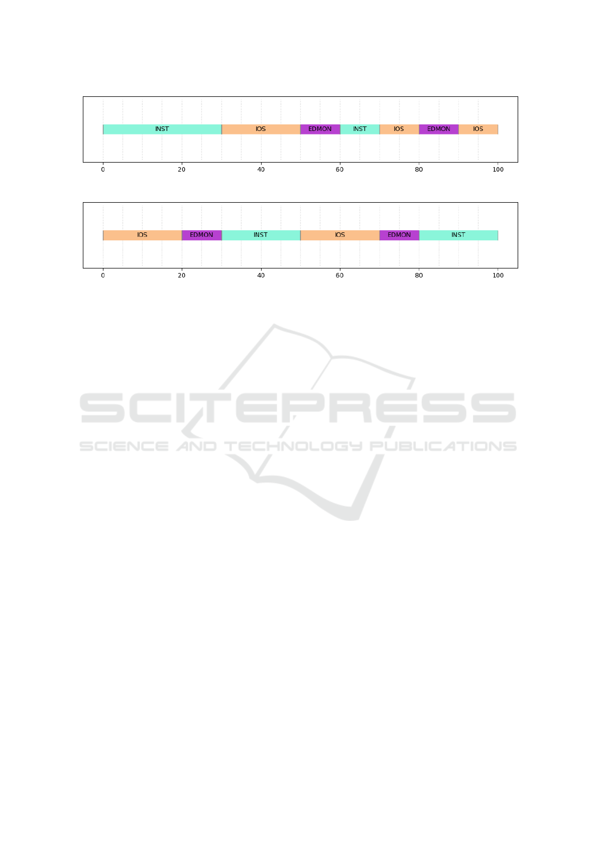
Figure 2: A valid schedule for instance NIMPH1.

Figure 3: An optimal schedule for instance NIMPH1.

zon h = 100 µs. We assume that IOS → EDMON is

the only precedence constraint and that INST is the

only critical partition with d

INST

max

= 40µs. Finally, the

minimum delay between two EDMON executions is

min

= 30µs. Both Figures 2 and 3 represent valid

schedules (i.e., a valid assignment of all tasks start)

with respect to these constraints. Note that consecu-

tive executions of the same partition are merged in the

Gantt chart. The schedule represented in Figure 2 is

valid but suboptimal (7 context switches), while the

schedule in Figure 3 is optimal (6 context switches).

3 NanoSatScheduler

We chose to tackle the NIMPH cyclic task schedul-

ing problem using Constraint Programming meth-

ods. We implemented NanoSatScheduler using IBM

ILOG CP Optimizer commercial solver. There are

two main reasons for this choice. First, CP Opti-

mizer has shown great results on a variety of schedul-

ing problems through the years (Laborie et al., 2018).

This solver is also simple to use, with dedicated li-

braries such as docplex for Python to build CP mod-

els (IBM, 2023). CP Optimizer provides global con-

straints and variable types, that make the modeling of

complex problems an intuitive process, especially for

scheduling.

We decided to implement two different models

to compare the performance of two modeling ap-

proaches for the NIMPH cyclic task scheduling prob-

lem. The ﬁrst model is called NanoSat and uses

only classical integer variables and no global con-

straints. Model NanoSatGlobal takes advantage of the

scheduling features of CP Optimizer (particular vari-

able structures and global constraints).

We ﬁnally developed an iterative method to insert

tasks of a given partition of the base instance to max-

imize the use of the schedule time, while taking the

context switches penalties into account.

3.1 NanoSat

Our ﬁrst constraint model aims to tackle the NIMPH

cyclic task scheduling problem only using simple

constraints and integer variables. Hence, it is possible

to implement it in any constraint solver. For NanoSat,

we deﬁne the following variables:

∈ [0, h] i = 1..N, j = 1..M

Start (8)

∈ [0, h] i = 1..N, j = 1..M

End (9)

∈ [0, 1] i = 1..N, j = 1..M

CS (10)

Start variables (8) are the start times for the j-th

occurrence of partition i. These are the only decision

variables, and a valid assignment for all start variables

is a solution. Task end times can be calculated from

the task starts and the constant task durations. End

variables (9) are only here for the sake of model clar-

ity. The tasks must be scheduled between 0 and the

time horizon h, therefore the domain of the start and

end variables is restricted to [0, h]. Context switch

(CS) variables (10) are binary variables that indicate,

for each task, whether the end time of the current task

is not equal to the start time of the next task of the

same partition (i.e., a context switch is needed). As

we want to limit the waste of the OBC schedule time,

our objective is to minimize the number of these con-

text switches under the following constraints:

min

∑

i=1

∑

j=1

(11)

ICORES 2024 - 13th International Conference on Operations Research and Enterprise Systems

280

= s

+ δ

i = 1..N, j = 1..M

(12)

≤ s

′

or s

≥ e

′

(i, j) ̸= (i

′

, j

′

) (13)

≤ s

j+1

i = 1..N, j = 1..M

-1 (14)

j+1

− s

≤ d

max

i : P

∈ C, j = 1..M

-1 (15)

h + s

− s

≤ d

max

i : P

∈ C (16)

j+1

− s

≥ d

min

j = 1..M

-1 (17)

h + s

− s

≥ d

min

(18)

= 1 or e

= s

j+1

i = 1..N, j = 1..M

-1 (19)

= 1 i = 1..N (20)

≤ s

(A, B) : A → B = E

′

(21)

≤ s

or e

≤ s

i = 1..N, j = 1..M

k = 1..M

(i, j) ̸= (A, k)

(i, j) ̸= (B, k)

(A, B) : A → B = E

′

(22)

Constraint (12) just deﬁnes the end of the tasks to

their start plus their duration. Constraint (13) forbids

the overlapping of any pair of tasks, as the OBC can

only execute one partition at the same time. The oc-

currences of the same partition are time-ordered (14)

for two reasons. First, the next constraints (15–22) are

easier to express if the tasks are ordered, which im-

proves model clarity. But more importantly, it elim-

inates a lot of symmetric solutions that could impact

the solving performance.

Constraint (15) states that the difference between

the start times of two consecutive critical tasks should

not exceed the maximum delay allowed for this par-

tition. Constraint (16) handles the side effect of the

transition between two cycles, as the schedule will be

restarted at the time horizon. In the same manner, the

minimum delay between two calls of EDMON parti-

tion is ensured with constraints (17–18).

We need to force the context switch variable c

0, if and only if task (i, j + 1) starts exactly at the end

time of the current task (i, j) (i.e., we can merge tasks

(i, j) and (i, j + 1) in the schedule). Constraint (19)

ensures that either c

is equal to 1 or the start time

of the occurrence j + 1 of partition i is equal to the

end time of the previous occurrence. As our objective

is to minimize

∑

i=1

∑

j=1

, the solver will set c

0 if the other condition is true, and c

will be forced

to 1 otherwise. The last task of every partition will

necessarily induces a context switch, so we set the

last context switch variable to 1 (20).

Our precedence graph G(V, E) states that for each

arc A → B in the precedence graph, only a task of

Figure 4: New simpliﬁed precedence graph with predeces-

sor partition split.

partition A can be the direct predecessor of a task of

partition B. In other words, no task of partition C ̸= A

can be inserted in the middle of a sequence AB. To

satisfy a precedence constraint A → B, we must have

at least as many tasks of type A as tasks of type B.

More generally, if we have n precedence constraints

for the same predecessor, e.g., A → B, A → C, ... the

number of predecessor tasks must be greater than or

equal to the number of successor tasks. As the tasks

within the same partition are interchangeable, we can

assign any task of the predecessor partition to be just

before any task of any successor partition, without im-

pacting the solution quality. Hence, for each partition

that is a predecessor of at least one other partition,

we can split the predecessor partition tasks set into n

distinct sets A

, A

, . . . for each successor, plus one

for the extra tasks of the predecessor partition. We

can now express the precedences with a bipartite di-

rected graph G(V

′

, E

′

) with only distinct pairs of par-

titions. We then force the k-th task occurrence of type

to be the direct predecessor of the k-th task occur-

rence of type P with constraints (21) and (22). The

ﬁrst constraint is a classical precedence constraint:

all tasks in a predecessor node must end before the

start of the corresponding task is the successor node.

The last constraint sets all other tasks to either end

before the predecessor task or to start after the suc-

cessor task for each precedence (i.e., each pair in our

new precedence graph G(E

′

)). As all partition sets

are time-ordered, we ensure strict precedences, while

maintaining the solution quality and breaking symme-

tries.

3.2 NanoSatGlobal

Model NanoSatGlobal uses the interval variables of

CP Optimizer, a structure dedicated to task modeling.

These variables have a start time, an end time and a

duration (that is ﬁxed in our problem). The main ad-

vantage of this kinds of variables is the synergy with

the sequence global constraint that allows us to rea-

son about the tasks as an ordered sequence rather than

a set of start times. We will use the notation t

for the

interval variable representing the task (i, j). Our vari-

Scheduling Onboard Tasks of the NIMPH Nanosatellite

281

ables are deﬁned as follows:

∈ [0, h] i = 1..N, j = 1..M

Task (23)

∈ [0, 1] i = 1..N, j = 1..M

CS (24)

Our interval variables start and end domains are

constrained within the time window [0, h] (23). We

model the context switches exactly as in the previous

model, and the objective function is the same:

min

∑

i=1

∑

j=1

(25)

However, our constraints are fundamentally dif-

ferent. Rather than working with the start dates of the

tasks, we use CP Optimizer scheduling global con-

straints on the sequence:

seq = sequence





, i



i=1..N, j=1..M



(26)

no overlap(seq) (27)

start of



j+1



− start of





≤ d

max

∀ i : P

∈ C, j = 1..M

-1 (28)

h + start of





− start of





≤ d

max

∀ i : P

∈ C (29)

start of



j+1



− start of





≥ d

min

∀ j = 1..M

-1 (30)

h + start of





− start of





≥ d

min

(31)

= 1 or



end of





= start of



j+1



∀ i = 1..N, j = 1..M

-1 (32)

= 1 ∀ i = 1..N (33)

type of prev



, A



∀ j = 1..M

, (A, B) : A → B ∈ E

′

(34)

In CP Optimizer, the sequence variable is a struc-

ture dedicated to task scheduling. We create such

a variable with all our tasks and we assign a differ-

ent type equal to the partition index for each (26).

This allows the use of global constraints on the inter-

val variables within the sequence, such as no overlap

constraint (27), that ensures that the tasks cannot run

at the same time. Just like in the previous section,

constraints (28, 29) ensure that the delay between two

tasks of the same critical partition is below d

max

and

constraints (30, 31) impose a minimum delay between

the start of two EDMON executions. The keyword

start of and end of respectively refers to the start and

the end of the interval variables. We constrain the

context switch variables (32, 33) as in the last model

(see Section 3.1). The global constraint type of prev

(34) is exactly what we need to express our strict

precedence constraints. This constraint forces the pre-

decessor of the current task to be of a speciﬁed type.

Note that we perform the same pre-processing step

described in Section 3.1 to express our precedence

graph G(V, E) as a perfect matching G(E

′

). There-

fore, for each arc A → B in G(E

′

), we assign a pre-

decessor of type A (i.e., from partition A) to each task

of partition B.

3.3 Lower Bound

To decrease the optimality proof computation time,

we calculate a lower bound lb on the number of con-

text switches for each instance. Indeed, our instances

have the following properties: A context switch is

needed for the last task of every partition. As the tasks

are ordered, the task starting just at the end of the last

task of a partition cannot be from the same partition;

A context switch is needed for every task of EDMON

partition as d

min

> δ

; Every task subject to a strict

precedence constraint will need a context switch (for

both predecessor and successor); Tasks subject to a

max delay constraint will need a minimum number of

context switches.

This last property is trickier. It is not obvious how

to compute the minimum number of context switches

for this last constraint, as it depends on the number

of tasks, the tasks’ duration, the time horizon and the

maximum delay allowed. To get this minimum num-

ber of context switches, we solve a simpliﬁed ver-

sion of the NIMPH cyclic task scheduling problem,

with only one partition, for each of these critical par-

titions. This simpler problem is solved to optimality

very quickly, so we can compute this minimum num-

ber of context switches for each critical partition as a

preprocessing step of NanoSatScheduler. The nota-

tion lb refer to the sum of all of these mandatory con-

text switches, so we can add the following constraint

to both NanoSat and NanoSatGlobal models:

∑

i=1

∑

j=1

≥ lb (35)

3.4 NanoSatIterative

Due to the various constraints on the NIMPH cyclic

task scheduling problem, it is very hard to manually

build instances that yield a valid solution that maxi-

mizes the useful schedule time. Moreover, it is not

useful to maximize the number of tasks for all kinds

of partitions. For instance, the number and duration

of the avionic partitions tasks are designed to ensure

the good behavior of the nanosatellite with respect to

a security margin, so maximizing these types of tasks

ICORES 2024 - 13th International Conference on Operations Research and Enterprise Systems

282

is unnecessary. On the other hand, the time allocated

to the scientiﬁc payloads should be maximized to im-

prove the scientiﬁc feedback.

To address this, we decided to relax the strict num-

ber of task constraints for one partition l, selected by

the user. We thus propose NanoSatIterative, a method

to ﬁnd the optimal useful schedule time, by jointly se-

lecting the number of tasks of partition l and schedul-

ing all the tasks. To maximize the useful schedule

time and keep the optimality guarantees, we perform a

dichotomic search on our objective:

∑

i=1

∑

j=1

−c

It is possible to compute a lower and an upper bound

on the number of tasks of type l. The lower bound

is the minimum number of tasks that are necessary

to reach the current objective, assuming an optimistic

number of context switches

, while the upper bound

is the number of tasks of type l before the problem

is trivially unsatisﬁable (i.e., the sum of the task du-

rations is greater than the time horizon). The lower

bound is updated at each objective step, and then

we iteratively add new tasks of partition l and try to

solve the NIMPH cyclic task scheduling problem with

a ﬁxed number of tasks using NanoSatScheduler or

NanoSatGlobal, until we reach either the upper bound

or we ﬁnd a feasible solution. According to the sat-

isﬁability of the problem with the current objective,

we update either the lower bound or the upper bound

of the useful schedule time. If a solution is found, we

also update the lower bound on the number of tasks of

type l with the current number of tasks. Note that we

cannot perform a dichotomic search on the number

of tasks as well, because a solution with more tasks is

not necessarily better than another solution with fewer

tasks but fewer context switches. If, at each step, we

can ﬁnd a valid solution or prove the unsatisﬁability

of the objective, the solution is optimal.

4 EXPERIMENTAL RESULTS

4.1 Instances

As the NIMPH mission is still in its development

phase, some of the real constraints for the NIMPH

cyclic task scheduling problem are still unknown

(e.g., tasks’ duration, exact number of occurrences,

minimum delay for critical partitions, etc.). To per-

form realistic and relevant experiments, the NIMPH

development team helped us create a base instance

with the expected values for each partition. As this

instance is subject to uncertainties and to deeply an-

We assume we can reach the lower bound presented in

Section 3.3.

alyze the performances of our approach, we gener-

ated 100 random instances based on the NIMPH nom-

inal instance (71 tasks from 10 distinct partitions, for

a time horizon h = 1s). We created these synthetic

instances by disturbing the original instance with a

Gaussian law (µ = 1, σ

= 0.3) for each uncertain

parameter. After deleting trivially unsatisﬁable in-

stances



∑

1=1

× M

> h



, we have a total of 98 in-

stances.

4.2 Results

We compare the two implementations NanoSat and

NanoSatGlobal of our model in CP Optimizer, and

the iterative method NanoSatIterative using both

NanoSat and NanoSatGlobal to solve the sub-

problems (with a ﬁxed number of partitions). We use

the following setup:

• Hardware: 13th Gen Intel® Core™ i7-1365U ×

12, 32 GB RAM.

• Solver: CP Optimizer 12.7.0 with docplex library

for Python.

• Time limit: 100 seconds (NanoSat, NanoSat-

Global), 1000 seconds (NanoSatIterative).

We can see in Table 1 that both NanoSat and

NanoSatGlobal are efﬁcient to solve NIMPH in-

stances, as feasible solutions are found very often and

a majority of instances can be solved to optimality

before 100 seconds. However, the use of CP Op-

timizer interval variables and sequence global con-

straints within NanoSatGlobal increases the resolu-

tion time and decreases the number of optimal so-

lutions on our instances, but this model is able to

prove the infeasibility of the few instances that are

not solved by NanoSat.

There is a higher contrast between these two ap-

proaches when they are integrated into NanoSatItera-

tive. Table 2 highlights the differences in terms of res-

olution time and proportion of optimal solutions be-

tween NanoSat and NanoSatGlobal within NanoSatIt-

erative. We can see that both methods improve the

useful schedule time, with a mean increase of 6% for

NanoSatIterative + NanoSat.

If the performances of both NanoSat and

NanoSatGlobal are globally satisfactory for the

NIMPH instances, such a performance gap between

those two models is hard to explain. A deeper analy-

sis of the models performance on bigger and more di-

verse instances is our main focus for the future work.

Scheduling Onboard Tasks of the NIMPH Nanosatellite

283

Table 1: Comparison of methods NanoSat and NanoSatGlobal: Mean resolution time; Number of instances solved; Number

of instances solved to optimality; Number of instances proved infeasible.

Method Mean time Nb. feasible Nb. optimal Nb. Infeasible

NanoSat 6.4s 94 94 0

NanoSatGlobal 33.1s 75 74 4

Table 2: Comparison of methods NanoSat and NanoSatGlobal within NanoSatIterative: Mean resolution time; Mean instances

solved to optimality; Mean useful schedule time; Mean upper bound on the useful time for the original instances (without

adding tasks).

Method Mean time Mean optimal Mean sched. use Mean original sched. use

NanoSatIterative+

NanoSat

58.1s 89.8% 88.5% 82.5%

NanoSatIterative+

NanoSatGlobal

786.5s 11.2% 83.1% 82.5%

5 CONCLUSION

We presented NanoSatScheduler, a tool suited for on-

board task scheduling in the context of nanosatellite

missions. Two versions of our software are compared,

and we highlighted that the use of CP Optimizer

global constraints is less effective than a classical

model for the NIMPH cyclic task scheduling problem,

while demonstrating the efﬁciency of both methods

to ﬁnd optimal schedules for NIMPH instances. We

also presented NanoSatIterative, a method to enhance

solution quality by iteratively inserting new tasks into

the instance and maximizing the useful schedule time.

Apart from improving experimental analysis,

there are still some interesting research directions re-

lated to the OBC task scheduling, in synergy with

NIMPH team needs. First, the iterative method could

be improved to handle multiple partitions, solving

a multi-objective problem of maximizing the use-

ful schedule time of each partition. NanoSatSched-

uler could beneﬁt from a Graphical User Interface,

with the possibility of dynamically modifying the in-

stances, to allow manual reﬁning from the NIMPH

team, while ensuring the feasibility or the optimality

of each new solution. A variant of the NIMPH cyclic

task scheduling problem with a variable time horizon

would be very interesting to investigate, as the useful

schedule time could be improved by reducing the time

horizon instead of adding new tasks.

REFERENCES

Balbastre, P., Masmano, M., and Morales, V. (June, 2021).

User manual. Technical Report fnts-xe-um-17b, Fent

Innovative Software Solutions.

CNES (2021). CNES project libraries – Nanolab Academy.

https://nanolab-academy.cnes.fr/en/janus.

Comer, D. and Fossum, T. V. (1987). Operating System

Design: Internetworking with Xinu. Prentice Hall.

IBM (2023). IBM Docplex documentation.

https://ibmdecisionoptimization.github.io/docplex-

doc/cp/index.html. Accessed on October 9th 2023.

Laborie, P., Rogerie, J., Shaw, P., and Vil

ım, P. (2018).

IBM ILOG CP Optimizer for scheduling: 20+ years

of scheduling with constraints at IBM/ILOG. Con-

straints, 23:210–250.

Landrea, T., Maignan, M., Risson, A., and Roux, G. (2018).

eciﬁcation mission NIMPH. ISAE-SUPAERO and

CSUT.

Li, C., Ding, C., and Shen, K. (2007). Quantifying the cost

of context switch. In Proceedings of the 2007 Work-

shop on Experimental Computer Science, pages 2–es,

San Diego, CA (USA).

Masmano, M., Ripoll, I., Crespo, A., and Metge, J. (2009).

XtratuM: A hypervisor for safety critical embedded

systems. In 11th Real-Time Linux Workshop, vol-

ume 9, Dresden (Germany).

Potts, C. N. and Kovalyov, M. Y. (2000). Scheduling with

batching: A review. European Journal of Operational

Research, 120(2):228–249.

Wikum, E. D., Llewellyn, D. C., and Nemhauser, G. L.

(1994). One-machine generalized precedence con-

strained scheduling problems. Operations Research

Letters, 16(2):87–99.

Windsor, J. and Hjortnaes, K. (2009). Time and space parti-

tioning in spacecraft avionics. In 2009 Third IEEE In-

ternational Conference on Space Mission Challenges

for Information Technology, pages 13–20. IEEE.

Yu, W., Hoogeveen, H., and Lenstra, J. K. (2004). Min-

imizing makespan in a two-machine ﬂow shop with

delays and unit-time operations is NP-hard. Journal

of Scheduling, 7:333–348.

ICORES 2024 - 13th International Conference on Operations Research and Enterprise Systems

284