Performance Evaluation of Polynomial Commitments for Erasure Code

Based Information Dispersal

Antoine Stevan

1 a

, Thomas Lavaur

1,2 b

, J

ome Lacan

1 c

, Jonathan Detchart

1 d

and

Tanguy P

erennou

1 e

ISAE-SUPAERO, Toulouse, France

University Toulouse III Paul Sabatier, Toulouse, France

{ﬁrstname.lastname}@isae-supaero.fr

Keywords:

Erasure Code, Polynomial Commitment, Distributed Storage.

Abstract:

Erasure coding is a common tool that improves the dependability of distributed storage systems. Basically,

to decode data that has been encoded from k source shards into n output shards with an erasure code, a node

of the network must download at least k shards and launch the decoding process. However, if one of the

shards is intentionally or accidentally modiﬁed, the decoding process will reconstruct invalid data. To allow

the veriﬁcation of each shard independently without running the decoding for the whole data, the encoder

can add a cryptographic proof to each output shard which certiﬁes its validity. In this paper, we focus on the

following commitment-based schemes: KZG

, aPlonK-PC and Semi-AVID-PC. These schemes perform

polynomial evaluations in the same way as a Reed-Solomon encoding process. Still, such commitment-based

schemes may introduce huge computation times as well as large storage space needs. This paper compares

their performance to help designers of distributed storage systems identify the optimal proof depending on

constraints like data size, information dispersal and frequency of proof veriﬁcation against proof generation.

We show that in most cases Semi-AVID-PC is the optimal solution, except when the input ﬁles and the

required amount of veriﬁcations are large, where aPlonK-PC is optimal.

1 INTRODUCTION

Erasure code is interesting in many applications like

distributed storage or real-time streaming. In the case

of distributed storage, a ﬁle F containing |F| bytes

is generally split into k shards of m elements which

are combined to generate n encoded shards (n ≥ k).

These shards are then distributed on different storage

servers, nodes or pairs. When a user wants to recover

F, they must download any k shards among the n ones

and apply the decoding process to reconstruct the ﬁle.

One potential issue in this scheme is that some

shards can be corrupted or intentionally modiﬁed by

their server. In this case, the reconstructed ﬁle does

not correspond to the initial ﬁle.

Even if it is generally easy to detect this event,

for example by verifying that the hash of the ﬁle cor-

https://orcid.org/0009-0003-5684-5862

https://orcid.org/0000-0001-9869-5856

https://orcid.org/0000-0002-3121-4824

https://orcid.org/0000-0002-4237-5981

https://orcid.org/0009-0002-2542-0004

responds to a hash initially published when the data

is put into this system, it can be time-consuming and

difﬁcult to identify the corrupted shard(s) and replace

them with non-corrupted ones.

This issue can be solved by using cryptographic

proofs. The principle is to publish a commitment of

the ﬁle and to add a proof linked to this commitment

to each encoded shard.

This scheme is of interest for trustless distributed

storage systems using erasure codes, such as peer-to-

peer distributed ﬁle systems (Daniel and Tschorsch,

2022). Also, large data availability systems that

store the data associated to rollups of next-generation

blockchains like Ethereum (Wood et al., 2014) or

even code-based low storage blockchain nodes (Per-

ard et al., 2018) may also be improved.

In this paper, we will focus on polynomial com-

mitment schemes taken from the most recent cryp-

tographic systems, that prove that a shard was really

encoded from the initial shards of the ﬁle. We assume

that the initial data is arranged in an m × k matrix of

ﬁnite ﬁeld elements. A shard corresponds to a column

and thus the data is split into k shards. The encoding

522

Stevan, A., Lavaur, T., Lacan, J., Detchart, J. and Pérennou, T.

Performance Evaluation of Polynomial Commitments for Erasure Code Based Information Dispersal.

DOI: 10.5220/0012377900003648

Paper published under CC license (CC BY-NC-ND 4.0)

In Proceedings of the 10th International Conference on Information Systems Security and Privacy (ICISSP 2024), pages 522-533

ISBN: 978-989-758-683-5; ISSN: 2184-4356

process combines these shards row-by-row to produce

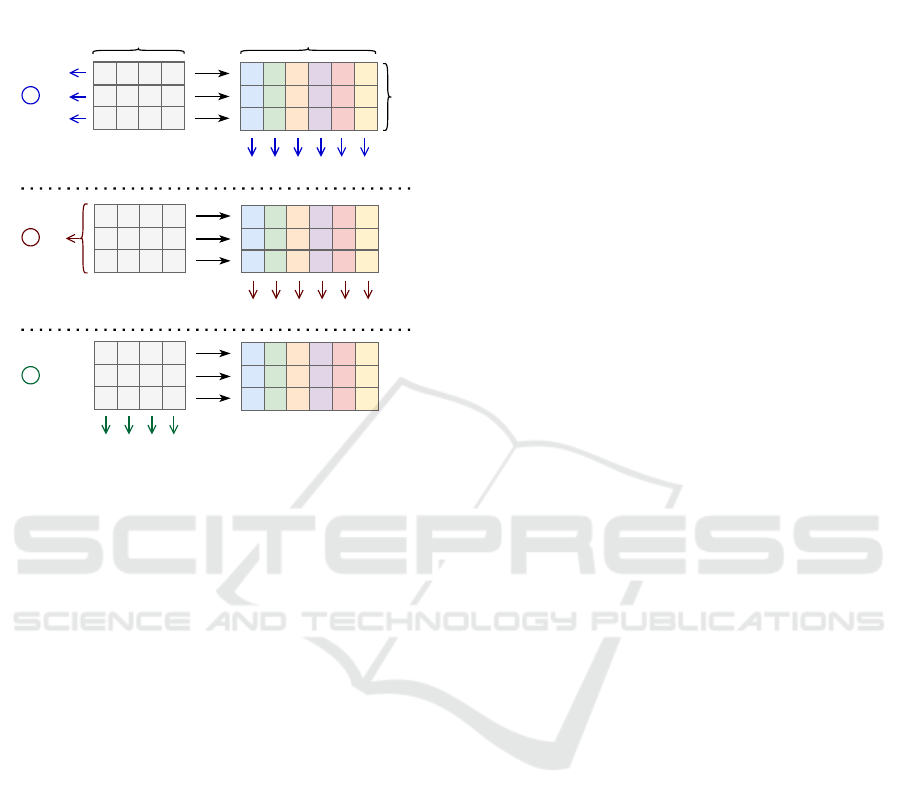
n encoded shards. Figure 1 presents in a simpliﬁed

way the three considered schemes.

encoding

k n

Figure 1: Polynomial commitment schemes for erasure

codes: It is assumed that the input data is the same for all

schemes, depicted with the same gray matrix of elements

to the left. The n output shards are shown with different

colors, one for each column, and are thus the same for each

scheme: ➀ KZG

will commit the m lines and generate one

proof for each of the n output columns, ➁ aPlonK-PC will

commit a single commit for the whole data, with a proof

for that commitment as well as one proof for each of the n

shards and ➂ Semi-AVID-PC will commit the k columns

and does not require any proof.

Rationale. The ﬁrst naive solution is the well-

known Kate-Zaverucha-Goldberg (KZG) tech-

nique (Kate et al., 2010) detailed in Section 2. Then

KZG

is a straightforward non-interactive extension

to any number of polynomials. Its commitment is

a vector of m KZG commitments and a witness,

computed as the aggregation of m KZG witnesses,

and is joined to each encoded shard. Next comes

aPlonK-PC which reduces the commitment of

KZG

to a constant size. It is a part of the veriﬁable

computation protocol aPlonK (Ambrona et al., 2022).

In counterpart, the generation and the veriﬁcation of

the witnesses is more complex. Finally Semi-AVID-

PC from Semi-AVID-PR (Nazirkhanova et al., 2021)

is of interest because it does not use any proof and

is a lot simpler than all the other techniques. The

commitment is a vector of k KZG commitments. The

veriﬁer will use the additive homomorphic property

of the commitments to verify that a given shard is

indeed a linear combination of the source shards.

Even if a quick analysis of Figure 1 seems to indi-

cate that the main difference between these solutions

concern the commitment, they strongly differ in sev-

eral points. First, for sake of simplicity, we have de-

noted all the proofs with the same notation π

, but in

reality their sizes are very different from one scheme

to another. Moreover, for each scheme, three algo-

rithms can be identiﬁed : the commitment generation,

the proof generation and the proof veriﬁcation. Since

the mathematical tools used by each technique are dif-

ferent, their complexities strongly vary.

Contributions. In this paper, all these techniques

are compared in terms of time complexities and

proof lengths. We have fully implemented each of

these algorithms with the library Arkworks (arkworks

contributors, 2022) at https://gitlab.isae-supaero.fr/

dragoon/pcs-fec-id and conducted benchmarks on the

same architecture for a large set of parameters. The

obtained results are then analyzed and should help

making the best choice of mechanisms according to

the constraints of a given system.

This analysis should be of interest for the de-

signers of distributed storage systems, especially re-

garding new data availability systems for blockchains.

Another application could be a swarm of military

drones that need to store and share trusted data in an

untrusted and potentially adversarial environment.

Outline. First, in Section 2, a broad overview of

Erasure Codes and commitment-based protocols will

be given. The next Section 3 will be dedicated to

the Rust implementation that goes alongside this pa-

per, which part of the algorithms have been discarded

and why, as well as which parts have been kept and

tweaked to the applications put forward in this docu-

ment. Then, the performance of the three main algo-

rithms and protocols selected here, KZG

, aPlonK-

PC and Semi-AVID-PC will be compared in Sec-

tion 4, in which 4 decision criteria have been iden-

tiﬁed. Section 5 will propose a discussion about a

few real-world use cases related to the applications

introduced earlier and determine which scheme ap-

pears best in each one of them. Finally, Section 6 will

conclude this paper.

2 BACKGROUND AND RELATED

WORK

All operations described in this paper are performed

on a ﬁnite ﬁeld F of large prime order p.

Performance Evaluation of Polynomial Commitments for Erasure Code Based Information Dispersal

523

The concept of Information Dispersal of a ﬁle with

erasure code was ﬁrst introduced by (Rabin, 1989)

and the validity of the distributed shards was ﬁrst

considered by (Krawczyk, 1993). In this paper, we

analyse some mechanisms providing the veriﬁability

property of the coded shards.

2.1 Erasure Coding

In distributed storage systems, whether it is on hard-

ware, on local networks or with the World Wide Web,

there will be issues and mishaps. Nodes can have

trouble reaching and communicating between each

other. Communication channels can introduce poten-

tially irrecoverable errors. Nodes and their data can

become unavailable and, in a worst-case scenario, the

network could end up split into multiple subnetworks

that are unable of communicating.

With all these potential risks, the goal would be

to be able to recover the data of interest even if the

network falls in anyone of the cases above.

One naive way of doing this is introducing redun-

dancy to the data by duplicating the whole sequence

of bytes. This has the beneﬁt of making the network

more resilient -if one or more nodes storing the data

are lost, it might still be possible to recover the whole

data by querying another node. However, this clearly

introduces a big overhead because the storage capac-

ity must be multiplied by a factor that is the redun-

dancy requirement of the system.

Another way of achieving the same level of re-

silience without storing the same data a lot of times is

to use Erasure Coding, one of them being the Reed-

Solomon encoding.

Such a scheme uses two parameters k and n, or

alternately k and ρ where ρ is the code rate of the

encoding and n =

. Given some data, the algorithm

consists in splitting the bytes into k shards of equal

size, applying a linear transformation, namely a k ×

n matrix multiplication to generate n news shards of

data. Each one of these shards is a linear combination

of all the k source shards. The biggest advantage of

this technique is that one needs to retrieve only any k

of the total n shards to recompute the original data.

With Erasure coding and especially Reed-

Solomon codes, a network which is more resilient to

losing nodes and copies of the data can be created,

while keeping low overhead and redundancy. How-

ever, such a code never ensures the integrity of the

data, i.e. there is no guarantee as the receiving node

that the shard has been indeed generated as a linear

combination of the source data...

The simplest solution to implement this scheme

is to use Merkle trees (Merkle, 1988) built from the

encoded shards. The commitment of the ﬁle is the

Merkle root and the proof joined to each encoded

shard is their Merkle proof. However, this proof just

certiﬁes that the shard was included in the computa-

tion of the Merkle root, but not that it is the result of

an encoding process. A node querying the network

will need to rely on the good behaviour of the Merkle

prover and could be easily tricked. Furthermore, gen-

erating additional proven shards from the data would

require to reconstruct a full Merkle tree whereas the

methods explored in the rest of this paper allow to

craft a single additional shard with a single proof.

To this end, cryptographic schemes can be used to

add hard-to-fake guarantees that any of the n shards

of data has indeed been generated as a linear com-

bination of the k source shards. The following sec-

tion will be dedicated to introducing a particular class

of such cryptographic schemes known as Polynomial

Commitment Schemes or PCS.

2.2 Polynomial Commitments Schemes

In the rest of this paper, we introduce a few notations:

H is a one-way hash function that takes an input se-

quence of bytes of any length and computes a ﬁxed-

size output, e.g. SHA256. G

, G

and G

are additive

sub-groups associated with a chosen elliptic curve. E

is a bilinear pairing operation that maps elements of

× G

to G

Polynomial Commitment Schemes are generally

used as an interactive process between a prover and a

veriﬁer. Later, this interaction can be removed with

the Fiat-Shamir transform (Fiat and Shamir, 1987).

Because the non-interactive counterparts of each al-

gorithm has been implemented alongside this paper,

the schemes will be presented with the non-interactive

transformation already applied.

Let us assume a prover Peggy has a polynomial

P and she wants to prove to a veriﬁer called Victor

that she knows the value of such a polynomial when

evaluated at a point x.

Peggy wants to convince Victor with overwhelm-

ing probability that she knows the value of P evalu-

ated at some point x, i.e. P(x) = y, without reveal-

ing any information to Victor about the polynomial

P itself. Moreover, she wants this operation to be

lightweight and easy to create and verify.

2.2.1 KZG and KZG

The ﬁrst protocols that have been studied were the

KZG PCS of (Kate et al., 2010) and its multi-

polynomial extension introduced in (Boneh et al.,

2020) and (Gabizon et al., 2019) that will be called

ICISSP 2024 - 10th International Conference on Information Systems Security and Privacy

524

KZG

in the rest of this paper, to clearly denote it is

a quite straightforward extension of regular KZG.

The motivations behind starting with these two al-

gorithms are the following:

• when Peggy constructs a proof for one of the n

shards of data, she will be evaluating the polyno-

mial P on predeﬁned points, e.g. 1, 2, ..., n, and it

is straightforward to show that this computation is

equivalent to performing a Reed-Solomon encod-

ing with a Vandermonde matrix.

This is very interesting because, while Peggy is

creating the proof π

of a given shard α she can

reuse the polynomial evaluations and get a Reed-

Solomon encoding for free.

• the proof size is constant and does not depend on

the degree of the polynomial P.

• the proof is fast to generate and is also fast for

Victor to verify.

The KZG protocol is the simplest one to explain:

• Peggy and Victor generate a trusted setup to-

gether (Bowe et al., 2017), i.e. the d + 1 pow-

ers of a secret number τ encoded on an elliptic

curve, [1]

,[τ]

,[τ

]

,...,[τ

]

where d = deg(P)

and [x]

:= x × G

where G

is a generator of the

elliptic curve group.

• Peggy constructs a commit of the polynomial P,

i.e. an evaluation of P on τ using the trusted

setup. Note that there is no need to know the ac-

tual value of τ because the encoding on an elliptic

curve is homomorphic: [a + b]

= (a + b)G

+ bG

= [a]

+ [b]

• then Peggy can construct a proof π

that links the

polynomial P to the shard of RS data.

• ﬁnally Victor will be able, by using a part of the

trusted setup and some operations on the elliptic

curve, to verify the integrity of the encoded shard.

This whole protocol ensures that the shard of en-

coded data has been generated as an evaluation of a

polynomial whose coefﬁcients are the rows of the k

source shards.

However, this KZG protocol is limited to a single

polynomial. In the following of the paper, larger and

larger data will be considered. Once encoded as ele-

ments of the chosen ﬁnite ﬁeld, the bytes could be in-

terpreted as a single polynomial. However, this naive

approach would require k to be very large and thus

will slow down the decoding process. The approach

that will be used in this paper is to arrange the el-

ements in an m × k matrix where k is the encoding

parameter and m is the number of polynomials. If the

size of the data is not divisible by k, padding can be

used. This will help keep the value of k lower and

leverage the aggregation capabilities of KZG

A naive approach would be to run a different KZG

on each one of the m lines and thus create m commits

in total and m proofs by shard of encoded data.

This is clearly not scalable for a particular value

of k when the size of the data gets larger and this is

where KZG

starts to shine.

In this paper and section, the multipolynomial

KZG protocol from (Boneh et al., 2020), which is in-

teractive, has been adapted to a non-interactive setup,

and will be called KZG

KZG

starts just as KZG with a setup and com-

mitting the m polynomials:

= [P

(τ)]

= P

(τ)G

, for i = 1, .. ., m (1)

However, instead of constructing one proof for

each polynomial (P

)

1≤i≤m

, Peggy will aggregate the

m polynomials into a single polynomial called Q as a

uniformly random linear combination of the (P

) and

then she will run a normal KZG on Q.

• for the non-interactive part of the protocol, the

prover hashes the evaluations of all the polyno-

mials on the shard evaluation point, α

r = H(P

(α)|P

(α)|...|P

(α)) (2)

• Peggy computes the polynomial Q(X) as

Q(X) =

∑

i=1

i−1

(X) (3)

• ﬁnally the proof π

of shard α is computed as a

KZG opening on the point α



Q(τ) − Q(α)

τ − α



(4)

On the other side, Victor will have to compute the

same random linear combination from the shard of

encoded data he received and compare it to the com-

bination of all the commitments. He has access to the

commitments from Equation 1, the shard (s

)

1≤i≤m

and the proof π

from Equation 4:

• the veriﬁer computes the same non-interactive

hash as in Equation 2

r = H(s

|...|s

) (5)

• Victor recomputes Q(α) with r and the shard as

y =

∑

i=1

i−1

(6)

• the veriﬁcation also requires to compute the com-

mitment of Q(X)

c =

∑

i=1

i−1

(7)

Performance Evaluation of Polynomial Commitments for Erasure Code Based Information Dispersal

525

• ﬁnally, Victor can perform a check with 2 pairings

E(c − [y]

,[1]

) = E(π

,[τ − α]

) (8)

With this scheme, some performance is lost in the

proof and veriﬁcation steps, because both Peggy and

Victor have more work to do, but a lot is gained in

proof sizes, going down from m proofs to a single one.

It has been seen that KZG

introduces a proto-

col that can scale up KZG when the size of the data

grows. However, the number of commits is still grow-

ing, which can become large for very big data and

values of |F|.

2.2.2 aPlonK-PC

The next protocol of interest is the PCS part of

aPlonK in (Ambrona et al., 2022).

Without the arithmetization part of aPlonK, the

protocol basically starts in the same way as in KZG

Peggy will commit all of the m polynomials, generat-

ing m elements of the elliptic curve. One proof is also

constructed for each shard of encoded data. This sub-

set of the aPlonK protocol will be called aPlonK-PC

in this document.

The improvement comes in the reduction of the

size of the overall commitment. Peggy won’t be send-

ing m commits, but rather a single meta-commit with

a proof that this commit was indeed generated thanks

to the m polynomial commits. This proof is gener-

ated through an expensive folding algorithm similar

to the one of Inner Product Arguments (B

unz et al.,

2018) but with elements of G

instead of elements of

F which will required a lot of pairing operations on

the elliptic curve.

This algorithm will fold the m commits into a sin-

gle one, alongside a proof of size O(log(m)).

So far, KZG has been made more scalable with

KZG

at the cost of more commitments and KZG

has been made more scalable with aPlonK-PC by

reducing the number of commitments at the cost of

harder to generate proofs, longer veriﬁcation and a

slightly bigger proof and trusted setup but which only

scale with the log(m).

But is the generation of proofs required at all to

reach the same level of security? The next section

will show that it is not and that some proof time and

storage capacity can be trade for much smaller proofs

and algorithmic complexity.

2.3 Semi-AVID-PC

Up until now, to prove some input data and generate

encoded shards, Peggy has been putting all the bytes,

once converted to elements of the ﬁnite ﬁeld, into an

m × k matrix. Then she committed the rows of the

matrix, constructing m commits and one proof per

column, i.e. by aggregating elements of the elliptic

curve into one per shard.

In (Nazirkhanova et al., 2021), the authors in-

troduce a protocol called Semi-AVID-PR which does

commit the polynomials in an orthogonal way. In-

stead of committing each one of the m lines, each

column of the matrix will be interpreted as its own

polynomial and committed. Peggy does not have

to do anything else apart from evaluating the row-

polynomials to generate the encoded shards of data.

Note that here, the prover does not prove individ-

ual polynomial evaluations like KZG

and aPlonK-

PC did, rather the linear combination of commits

and thus of the underlying shards. The interest of

the polynomial evaluations is that they prove that the

encoding corresponds to a Reed-Solomon encoding

which ensures that the ﬁle can be recovered with any

k shards among the n ones. This is not the case for

the simple linear combination scheme which could

need more than k shards to recover the ﬁle. How-

ever, if the veriﬁer checks that the coefﬁcients of the

linear combination corresponds to the powers of the

shard index, the Reed-Solomon encoding is also ver-

iﬁed . As the focus here is only on the commitment

part of Semi-AVID-PR and to stay consistent with the

other schemes which are true polynomial commit-

ments, this new and last scheme will be called Semi-

AVID-PC.

The job of Victor is quite simple and fast as well.

Because the commit is homomorphic, the linear com-

bination of the commits of some polynomials is equal

to the commit of the same linear combination of the

same polynomials. As the shard of encoded data Vic-

tor would like to verify has been generated as a known

linear combination of the original source data shards,

it is very easy for him to ﬁrst compute the commit of

the shard he received by interpreting the bytes as the

coefﬁcients of a polynomial, then compute the linear

combination of the k commits that Peggy sent him and

ﬁnally check that the commit of this polynomial is in-

deed equal to the expected linear combination of the

commits from Peggy.

As one can see in the previous paragraphs, both

the work of Peggy and Victor are very simple and fast,

only k commits for Peggy, and one commit and a lin-

ear combination of elements of the elliptic curve for

Victor. Moreover, if the protocol can keep the value of

k as low as possible, the size of the proof will remain

very small and constant with the size of the data.

The major drawback of this scheme is that Victor

needs to have access to the full trusted setup to ver-

ify one given shard of encoded data, whereas KZG

ICISSP 2024 - 10th International Conference on Information Systems Security and Privacy

526

and aPlonK-PC required only one or at most a few

elements of the elliptic curve. Here Semi-AVID-PC

needs to store or retrieve the m ﬁrst elements of the

trusted setup which will get bigger and bigger when

the data becomes larger for a given ﬁxed value of k.

3 IMPLEMENTATION

All the algorithms introduced in Sections 2.2 and 2.3

have been implemented on the ISAE-SUPAERO Git-

Lab

These schemes have been implemented using the

Arkworks library written in Rust (arkworks contribu-

tors, 2022). They can all work over several pairing-

based elliptic curves. In Section 4, we show some

results based on the BLS-12-381 elliptic curve.

Note that, thanks to the design of the Arkworks li-

brary, another curve could be easily switched to, e.g.

another common pairing-friendly curve is BN-254.

However, one single curve has been chosen because

changing to another one would affect all the proving

schemes in the same exact way as they all use the

same curve and the same kind of operations on said

curve. As an example, switching from BLS-12-381

to BN-254 would roughly decrease both the time and

the sizes of everything by 30% at the cost of a few bits

of security, which might become a decision level for

some applications. This means that measuring per-

formance on any of the curves would lead to the same

conclusions as our goal is to compare the schemes be-

tween each other and not absolutely.

For aPlonK-PC, the only noticeable optimization

that has been added to the implementation as com-

pared to the algorithms presented in the paper of (Am-

brona et al., 2022) is the computation of the powers of

the random r scalar element which is done recursively

to avoid computing many times the same power of r

over and over.

In (Nazirkhanova et al., 2021), the authors use a

polynomial interpolation and the FFT to make some

computations faster. To the best of our knowledge,

the interpolation is not required. Instead of seeing the

k columns of the input data as evaluations of the tar-

get polynomials, the same ﬁnite ﬁeld elements can be

directly interpreted as the coefﬁcients of the polyno-

mials, saving k polynomial interpolations.

Furthermore, the FFT does not appear to be of par-

ticular interest for the applications in the scope of this

paper. In (Nazirkhanova et al., 2021), the authors say

that the performance bottleneck the FFT solves starts

to make sense when the polynomials are evaluated on

https://gitlab.isae-supaero.fr/dragoon/pcs-fec-id

n points when the global system under study is big,

namely when n ≥ 1024. With the analysis of the per-

formance in the next section, the FFT was discarded

because the values of k and n never go high enough

for the FFT to have a signiﬁcant impact for the price

to pay to use it.

Related to FFTs and optimizing the energy cost of

many computations that could run in parallel, multi-

threading has not been implemented for the same rea-

sons as for the curve switch explained above: en-

abling multi-threading would beneﬁt all the schemes

in the same way because they all work in the same

manner, i.e. a loop with n rounds to generate n shards

and proofs or a loop with k rounds to verify k shards,

so the comparison between the schemes would not

change with that new feature enabled, the times are

expected to all decrease.

Lastly, one of the main contributions regarding the

algorithms themselves is that the whole proof systems

have not been implemented as-is but rather the pro-

tocols have been tailored to the needs of the appli-

cations in the scope of this paper by removing un-

necessary parts. When implementing aPlonK-PC

from (Ambrona et al., 2022), the whole arithmetiza-

tion part of the protocol which is useful when build-

ing a full SNARK circuit has been discarded. How-

ever, in the applications of this paper, the polynomi-

als to prove are already available, so there is no need

to create arithmetic circuits to convert any general

computation to polynomials. As for Semi-AVID-PC

from (Nazirkhanova et al., 2021), the signature and

proof part of the whole protocol, which is focused on

rollups for the Ethereum blockchain and data avail-

ability sampling as their main applications, has been

taken out and the committing of data columns, which

is enough to prove the integrity of data in the applica-

tions put forward in this paper has been kept.

4 PERFORMANCE EVALUATION

The original papers of the three schemes present al-

gorithmic complexities. However, in the context of

advanced performance analysis including execution

times, asymptotic complexities and the O notation are

not enough to compare the real-world implementa-

tions.

In this section, the different schemes introduced

in Sections 2.2 and 2.3 are evaluated and compared

with varying data sizes. For each size, several sets of

parameters m and k were evaluated because the per-

formance of the various schemes strongly depends on

them. Section 4.1 studies the raw measurements and

how they were computed. Four performance criteria

Performance Evaluation of Polynomial Commitments for Erasure Code Based Information Dispersal

527

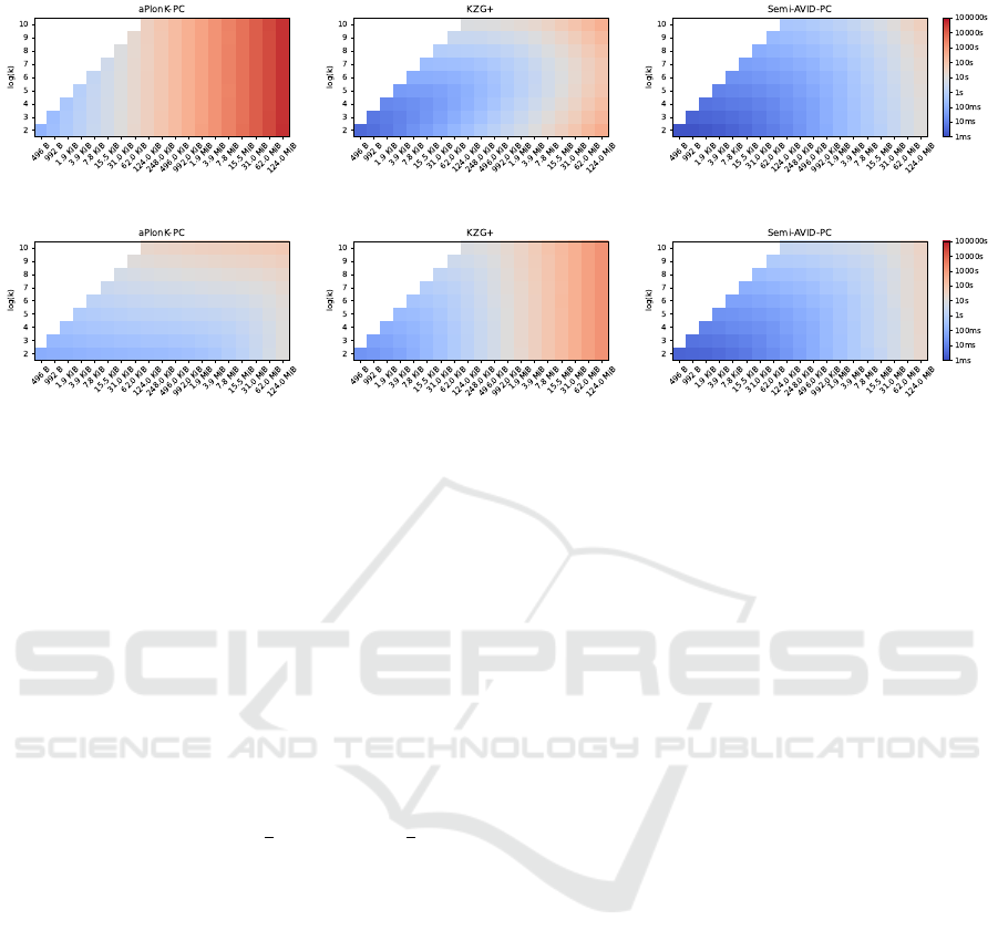
(a) Time to generate one commitment and n proofs

(b) Time to verify k shards

Figure 2: Execution times of proof generation and veriﬁcation for the three schemes, with different input data sizes and values

of k. All the scales are log for readability. The vertical axis shows log

(k) for convenience while the horizontal axis shows

the data size |F|. For any (k,|F|) pair, a square indicates the execution time using a colored log scale: blue squares indicate

short times and good performance while red squares indicate longer times.

that one might want to optimize for their particular

needs are detailed. A synthesis of the raw data will

be presented when k is ﬁxed (Section 4.2) and then

when k is chosen to optimize one of the criteria (Sec-

tion 4.3).

4.1 Raw Time Performance

In the rest of this section, the time it takes for each

stage of our protocols, i.e. the proofs, the veriﬁcation

and the decoding of shards, has been measured. The

code rate has been set to ρ =

such that n =

= 2k.

Regardless of the proving scheme, the end-to-end

process can be decomposed as follows, where items

written in bold have been measured:

• splitting the data: the |F| input bytes are arranged

in an m × k matrix of ﬁnite ﬁeld elements, 31 ∗

(m × k) = |F|, possibly with padding

• commitment: commit the whole data

• proof: construct a proof for each one of the n out-

put shards and disseminate them onto the network

• veriﬁcation: verify any k of the n output shards,

e.g after retrieving enough shards to theoretically

reconstruct the original data

• decoding: decode the k shards into the original

data by inverting a k × k matrix of curve elements

and then performing a k ×k matrix-vector product

A performance measurement campaign has been

conducted on a box with values:

• ranging from 4 = 2

to 1024 = 2

for k

• ranging from 496 B to 124 MiB, i.e. from 31 × 2

to 31 × 2

bytes, for the size of the data |F|

• spanning over KZG

, aPlonK-PC and Semi-

AVID-PC for the scheme

The resulting raw measurements can be found in

Figure 2. The top-left triangle of the whole square

of input parameters is white because these are impos-

sible parameter values, e.g. when the data contains

992 B, if k was set to 256, a polynomial of degree

255 would need to be proven where there are only

992/31 = 32 ﬁnite ﬁeld elements in the case of BLS-

12-381, thus 192 elements would be added as padding

and mostly padding bytes would be proven. So these

areas are shaded and considered as invalid.

For all schemes, both proof and veriﬁcation times

increase with k and data size |F|. For aPlonK-PC,

the value of k does not matter when k is small and

choosing k as small as possible leads to shorter veri-

ﬁcation times. For KZG

, there is an optimal region

in-between large and small values of k, both for the

proof and the veriﬁcation. Finally, Semi-AVID-PC is

the fastest in all aspects when k is small.

4.2 Systems Where k is Fixed

All schemes perform better with a small value of k,

but there are situations where the system requires a

larger k. For instance, in order to tolerate malicious

intrusion on one or more nodes without losing pri-

vacy, it is necessary that compromised nodes do not

host enough shards to decode any original data, which

is more difﬁcult with low values of k.

ICISSP 2024 - 10th International Conference on Information Systems Security and Privacy

528

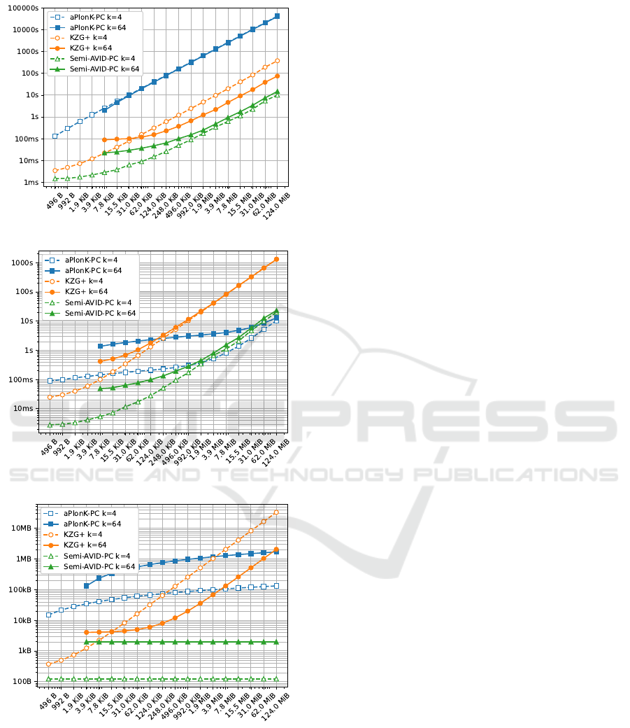
(a) Proof time for n shards

(b) Veriﬁcation time for k shards

Figure 3: Comparison of execution times and size over-

heads for the three schemes with a low k = 4 (dashed lines)

and a high k = 64 (solid lines). Note that the solid plots are

not drawn for small values of |F|. This is for the same rea-

son as for Figure 2: k is too big compared to |F|, thus a lot

of padding has to be used to have even a single polynomial.

We decided to omit these parameters.

Figure 3 compares the performance of the three

schemes for a low k = 4 and a high k = 64. Regard-

ing the proof time (Figure 3a), no matter the value

of k or the data size |F|, the schemes can be ordered

from fastest to slowest: Semi-AVID-PC, KZG

and

aPlonK-PC. Veriﬁcation time (Figure 3b) is more

complex: aPlonK-PC eventually becomes faster than

Semi-AVID-PC when |F| increases (1.9 MiB for k =

4 and 31 MiB for k = 64). For both values of k,

KZG

is largely outperformed by either Semi-AVID-

PC or aPlonK-PC. For proofs and commits sizes

(Figure 3c), Semi-AVID-PC is the smallest no matter

the value of k or the data size |F| because the overhead

is constant in k. KZG

and aPlonK-PC have much

larger overhead sizes, although aPlonK-PC eventu-

ally becomes smaller when |F| increases (248 KiB for

k = 4 and 124 MiB for k = 64).

4.3 Choosing the Optimal k

These general trends from Section 4.1 and 4.2 have

been further investigated: for each data size, scheme

and selected performance goals (proof time, veriﬁ-

cation time and proof size), the best (lowest) values

were identiﬁed among all values measured with dif-

ferent k values. The optimal k values are summarized

in Table 1 and the corresponding best values are plot-

ted on Figure 4. Figure 4a focuses on proof times: it

contains the proof times for KZG

, aPlonK-PC and

Semi-AVID-PC, for all optimal k values (optimal k

prf

for proof time, but also optimal k

vrf

for veriﬁcation

time and optimal k

for proof size; for Semi-AVID-

PC, the same k

opt

values optimizes the three perfor-

mance goals). Similarly, Figure 4b focuses on veri-

ﬁcation times, Figure 4c focuses on proof sizes and

Figure 4d focuses on decoding times.

For instance, for |F| = 7.8 MiB of data, KZG

best proof time plotted on Figure 4a is 4.6 s with

prf

= 64. For the same data size, aPlonK-PC best

proof time is 2544 s, with k

prf

= 32, and Semi-AVID-

PC best proof time is 625 ms with yet another dif-

ferent k

prf

= 4. In addition to the three best proof

time curves, Figure 4a shows the proof times obtained

with k

vrf

values optimizing the veriﬁcation time and

values optimizing the proof size.

To get a clear idea on which scheme to choose,

all four sub-ﬁgures must be used jointly. Continuing

the 7.8 MiB data example, Figure 4a showed that the

best proof time is 625 ms, obtained with Semi-AVID-

PC and k

prf

= 4. Keeping this value for k, Figure 4b

shows that Semi-AVID-PC veriﬁcation time is 1.1 s,

larger than aPlonK-PC’s 820 ms obtained with k =

vrf

= 4 to optimize veriﬁcation time, but lower than

any other; Figure 4c shows that proof size is 992 B,

Performance Evaluation of Polynomial Commitments for Erasure Code Based Information Dispersal

529

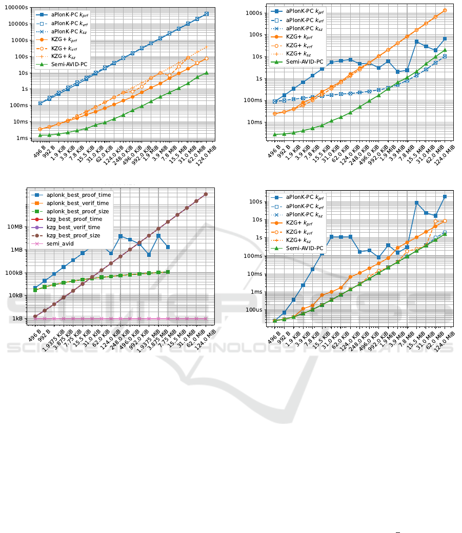
(a) Proof time for n shards

(b) Veriﬁcation time for k shards

(d) Decoding time for k shards

Figure 4: Times of proof, veriﬁcation and decoding operations for the three schemes, using optimal k values for three criteria:

optimizing proof time, veriﬁcation time and proof size; and size of proofs generated by the three schemes according to these

optimal k values. Note that for times, the vertical axes are different and use a log scale. The horizontal axis shows the data

size |F|. As proof and veriﬁcation are used in the context of FEC(k,n) encoding and decoding, proof is plotted for n shards,

and veriﬁcation/decoding are plotted for k shards. The exact values of k are not shown in these ﬁgures but are summarized

in Table 1. Note that in Figure 4c, all the KZG

curves overlap and in Figure 4d, the k

and k

curves of aPlonK-PC are

hidden behind the Semi-AVID-PC curves. All seven curves have been kept accross subﬁgures for consistency.

the lowest value; and Figure 4d shows that decoding

time is 91 ms, the lowest value again.

This quick ﬁrst analysis must be deepened accord-

ing to what needs to be optimized: execution time,

storage space, or both? Before a general application-

level analysis in Section 5, the four following sec-

tions present a separate performance comparison of

the three schemes for each measured data: proof time

(Section 4.3.1), veriﬁcation time (Section 4.3.2), de-

coding time (Section 4.3.3) and commit and proof

size (Section 4.3.4). These sections will take the data

size and the code rate of the encoding as input param-

eters imposed by the system and will help choose the

best scheme and the associated value of k.

4.3.1 Commit and Proof Generation

In this section, the schemes are compared when the

interest is in low proof times. The results can be found

in Figure 4a and the associated values of k are listed in

Table 1. For each scheme, data size |F| and optimiza-

tion criterion, Figure 4a shows the time to commit the

whole data once and to prove the n =

output shards.

Note that for Semi-AVID-PC, because k has the same

value for any given data size only one curve is plotted

to avoid curves overlapping.

For Semi-AVID-PC and aPlonK-PC, the three

curves are identical or very close, so optimizing for

a metric or another has no signiﬁcant impact. The

performance of KZG

varies a bit more depending

on the metric being optimized.

ICISSP 2024 - 10th International Conference on Information Systems Security and Privacy

530

Table 1: Optimal k value for each data size |F|, scheme and optimization goal. For brevity, each scheme is denoted with

only the ﬁrst letter, i.e. A for aPlonK-PC, K for KZG

and S for Semi-AVID-PC. The colors have been kept the same as in

Figure 4

Data size in B KiB MiB

496 992 1.9 3.9 7.8 15.5 31 62 124 248 496 992 1.9 3.9 7.8 15.5 31 62 124

prf

4 8 16 32 64 128 256 256 256 128 128 64 128 32 32 1024 512 256 1024

A k

vrf

4 4 4 4 4 4 4 4 4 4 4 4 4 4 4 4 4 8 8

4 4 4 4 4 4 4 4 4 4 4 4 4 4 4 4 4 4 4

prf

4 4 4 8 8 16 16 16 32 32 32 32 32 64 64 64 64 64 64

K k

vrf

4 4 4 4 4 4 4 4 4 4 8 8 4 4 16 8 4 128 64

4 4 4 4 4 4 4 4 4 4 4 4 4 4 4 4 4 4 4

S k

opt

4 4 4 4 4 4 4 4 4 4 4 4 4 4 4 4 4 4 4

aPlonK-PC is around 1 order of magnitude

slower than KZG

which is itself between 0.5 and

1 order of magnitude slower than Semi-AVID-PC,

which is by far the best scheme for this metric.

4.3.2 Shard Veriﬁcation

The veriﬁcation time will be optimized in Figure 4b.

As the reconstruction of a ﬁle of size |F| needs

k shards, the time to verify k shards has been mea-

sured. Note that, as the shards can be received asyn-

chronously, no batch method has been used, the time

needed to perform k successive shard veriﬁcations has

simply been computed.

As before, Semi-AVID-PC features a single curve

because all the values for k are the same regardless of

the metric optimized.

This ﬁgure is not as straightforward as the pre-

vious one from Section 4.3.1. For small ﬁle sizes,

KZG

and even more Semi-AVID-PC are far more

efﬁcient than aPlonK-PC is. However, thanks to

its logarithmic time complexity, aPlonK-PC quickly

catches up as the data size |F| gets bigger. Around 1

MiB, the time goes below the curve of Semi-AVID-

PC, making aPlonK-PC the go-to scheme when the

ﬁle is really big. Values of k are listed in Table 1.

4.3.3 Decoding File From k Shards

In this section, the focus will be low decoding times,

to allow frequent and fast full reconstruction of the

original data.

When a node veriﬁes k shards, it can decode them

in order to reconstruct the original data. The decoding

time has been measured function of the ﬁle size, and

the best k parameter for each scheme. If k is small, the

decoding time is negligible. This can be explained be-

cause most of the decoding complexity comes from

the fact that the reconstructing node needs to invert

a k × k matrix of elliptic curve elements. This opera-

tion has a complexity between O(k

) and O(k

) which

grows rapidly as k gets bigger.

The results for this metric optimization are shown

in Figure 4d and the associated values of k are again

listed in Table 1.

Note that, with this plot, the decoding time does

not really depend on the scheme and algorithm used

but rather completely on the value of k. Of course, the

value of k is a function of the scheme but this means

that, if two schemes have the same best k, then the

decoding times will be perfectly identical.

Because the optimal k stays small for both KZG

and Semi-AVID-PC, the decoding time associated to

these schemes is low compared to aPlonK-PC.

This metric has the lowest impact of all the four

metrics because, in general, the decoding time is neg-

ligible as compared to the proof and veriﬁcation times

for the whole data.

As before, note that, because k has the same value

for any given data size when looking at Semi-AVID-

PC only one curve has been plotted to avoid having

curves hidden behind each other.

4.3.4 Size Overhead of Commitments and Proofs

Function of k and |F|, the overhead of the commit-

ments and proofs needed to be stored in the shards

has been analyzed.

The theoretical proof and commit sizes have been

summarized in Table 2. This overhead for each

scheme is plotted against data size |F| in Figure 4c.

This ﬁgure shows the total size overhead of n com-

mits and n shards. The motivation is a network of

peers where each node of the network stores one of

the n shards, to disseminate the data, and one commit,

to be able to verify any of the shards when needed.

As expected, Semi-AVID-PC has the lowest

proofs + commitments size, because this scheme does

not have to construct any proof at all, and does only

rely on the homomorphic property of the commit op-

eration and asks the veriﬁer to do more work. When

|F| is big and thanks to its logarithmic complexity,

aPlonK-PC can have a lower overhead than KZG.

Another object that takes up more or less space

depending of the scheme and the size of the data is

the trusted setup and veriﬁcation keys.

As can be seen in the implementation, all schemes

require some form of trusted setup to construct the

commits and the proofs and veriﬁcation keys to verify

any encoded and proved shard.

Performance Evaluation of Polynomial Commitments for Erasure Code Based Information Dispersal

531

Table 2: Commit and proof sizes for a code rate ρ. On both BLS-12-381 and BN-254, and without any compression of ﬁeld

elements, G

= 2G

and G

= 12G

scheme commiment (c) proof (π) total

KZG

(c + π)

aPlonK-PC 1G

2(log

(m) + 1)G

+ 2G

+ 2 log

(m)G

Semi-AVID-PC kG

KZG

and Semi-AVID-PC use the same trusted

setup to prove the data, i.e. a list of the powers of a se-

cret element τ of the elliptic curve, KZG

needs m of

these powers whereas Semi-AVID-PC requires k of

them to commit the data. On the other hand, aPlonK-

PC needs the same m powers as KZG

does to com-

mit the data but also needs an additional element of

and a list of log

(m) elements of G

to construct

the Inner Product Argument. Even though the number

of elements may vary from one scheme to the other,

all the schemes require around O(m) elements of the

elliptic curve to commit and prove the whole data.

The biggest difference between the three schemes

under study comes with the veriﬁcation stage. KZG

needs a veriﬁcation key which is a single element of

and two elements of G

. aPlonK-PC requires a

bit more with an extra element of G

. In a nutshell,

both KZG

and aPlonK-PC asks for roughly a few

elliptic curve elements that grow with O(1) with the

data size |F|.

Because the Semi-AVID-PC veriﬁer needs to

compute the commit of the shard itself, he needs the

full m-long trusted setup, which will grow linearly

with the ﬁle size for a given value of k.

On any curve, the size of the trusted setup will

be equal to

|F|

|×k

elements, where |G

| is the size of

one element of G

, and thus

|F|

|×k

× |G

| =

|F|

, e.g.

for k = 4 and |F| = 124MiB, the size of the trusted

setup will be

or the whole data, i.e. 31 MiB of setup

elements.

5 DISCUSSION

The previous section showed that some compromises

have to be made. Most signiﬁcantly, when the data is

large, it is not possible to have both fast proving and

fast veriﬁcation. With big values of |F|, aPlonK-PC

and Semi-AVID-PC are competing, aPlonK-PC be-

ing better for veriﬁcation in the long run and Semi-

AVID-PC having lower proving time. In this sec-

tion, a few use-cases will be detailed and links will

be drawn between the raw analysis of Section 4 and

the applications introduced in Section 1.

In the ﬁrst scenario, suppose we want to prove a

ﬁle of size |F| = 7.8 MiB, but also want the veriﬁca-

tion to be as fast as possible. As seen in Figure 4b,

the best veriﬁcation time for this case is obtained by

aPlonK-PC in around 800 ms. However, with this

scheme, Figure 4a shows that the proof time reaches

around 2500 s. On the other hand, if we want the best

proof time for a given ﬁle of size |F| = 7.8MiB, the

best scheme is Semi-AVID-PC which will prove in

700 ms and verify in approximately 1 s. The time lost

in the veriﬁcation step is greatly gained and balanced

by the orders of magnitude of proof time.

Another scenario could be blockchain blocks

availability. Indeed, rather than duplicating the full

blocks on a large number of nodes, a solution could

be to encode the blocks as in Data Availability Sam-

pling (Perard et al., 2018) and adding a proof such

that the veriﬁers can detect errors in the shards be-

fore decoding them. In this scenario, the Ethereum

blockchain with an average block size of up to 32 MiB

and k = 1024 will be considered. Proof times and ver-

iﬁcation times for k = 1024 can be estimated from the

top lines of Figure 2a and Figure 2b. In this particular

case, there is no contest between the schemes: Semi-

AVID-PC is better (bluest) in proof time, veriﬁcation

time, size overheads and decoding time, by orders of

magnitude and always lower than 100 ms.

Finally, given the different operations, we can see

that the decoding time is negligible compared to the

proof time and the veriﬁcation time. Furthermore, we

can conclude that aPlonK-PC is the fastest scheme

for veriﬁcation for data sizes |F| larger than 31 MiB.

Semi-AVID-PC, even if a trusted setup is needed,

seems to be the best scheme for the proof genera-

tion and the proof size. The performance of this last

scheme in the veriﬁcation step is the best one for

smaller data sizes, and does not end up far behind

the best one, aPlonK-PC, for larger data sizes. This

makes this last Semi-AVID-PC scheme the overall

best of the three that have been studied.

6 CONCLUSION

This paper evaluates protocols that enhance the se-

curity of erasure code based distributed storage sys-

tems by allowing the early detection of corrupted data

shards. This is done by adding cryptographic proofs

to the data shards produced by an erasure code, using

ICISSP 2024 - 10th International Conference on Information Systems Security and Privacy

532

existing commitment schemes: KZG

, aPlonK-PC

and Semi-AVID-PC. Then, these output shards can

be veriﬁed individually before trying to decode the

full data.

We implemented the KZG

, aPlonK-PC and

Semi-AVID-PC commitment schemes using the Ark-

works cryptographic libraries. Their performance in

terms of execution time (generating or verifying cryp-

tographic proofs) and storage space (size of trusted

setup and generated proofs and commits) was then

analysed. In most cases Semi-AVID-PC is the op-

timal solution, except when the input ﬁles are large

and when the veriﬁcation time must be optimized. In

this case, aPlonK-PC is optimal.

For a designer of distributed storage systems, this

means that if a lot of individual shard veriﬁcations

must be done as compared to data addition and proofs

generation, aPlonK-PC should be considered as a

possible alternative to Semi-AVID-PC.

This can be the case for blockchains or their com-

panion rollups, where newly created blocks become

available only after numerous veriﬁcations are per-

formed by different nodes. This may also be the case

for systems where massive store-and-forward (gossip-

based protocols) is used for data dispersal, so that

only valid shards are stored on any node. In other

cases, Semi-AVID-PC is clearly the optimal solution.

Note, however, that it does not prove a Reed-Solomon

encoding, but simply a linear combination encoding,

which can be considered as weaker according to the

context.

Moreover, the performance costs to enhance the

security is acceptable. This allows for distributed stor-

age systems where only veriﬁed shards are stored, and

corrupted shards can be easily detected and discarded.

REFERENCES

Ambrona, M., Beunardeau, M., Schmitt, A.-L., and Toledo,

R. R. (2022). aPlonK : Aggregated PlonK from multi-

polynomial commitment schemes. Cryptology ePrint

Archive, Report 2022/1352. https://eprint.iacr.org/

2022/1352.

arkworks contributors (2022). arkworks zkSNARK

ecosystem. https://github.com/arkworks-rs. Ac-

cessed: 2023-10-18.

Boneh, D., Drake, J., Fisch, B., and Gabizon, A. (2020). Ef-

ﬁcient polynomial commitment schemes for multiple

points and polynomials. Cryptology ePrint Archive.

Bowe, S., Gabizon, A., and Miers, I. (2017). Scalable multi-

party computation for zk-SNARK parameters in the

random beacon model. Cryptology ePrint Archive,

Report 2017/1050. https://eprint.iacr.org/2017/1050.

unz, B., Bootle, J., Boneh, D., Poelstra, A., Wuille, P., and

Maxwell, G. (2018). Bulletproofs: Short proofs for

conﬁdential transactions and more. pages 315–334.

Daniel, E. and Tschorsch, F. (2022). IPFS and Friends: A

Qualitative Comparison of Next Generation Peer-to-

Peer Data Networks. IEEE Communications Surveys

& Tutorials, 24(1):31–52.

Fiat, A. and Shamir, A. (1987). How to prove your-

self: Practical solutions to identiﬁcation and signature

problems. pages 186–194.

Gabizon, A., Williamson, Z. J., and Ciobotaru, O. (2019).

PLONK: Permutations over lagrange-bases for oe-

cumenical noninteractive arguments of knowledge.

Cryptology ePrint Archive, Report 2019/953. https:

//eprint.iacr.org/2019/953.

Kate, A., Zaverucha, G. M., and Goldberg, I. (2010).

Constant-size commitments to polynomials and their

applications. pages 177–194.

Krawczyk, H. (1993). Distributed ﬁngerprints and secure

information dispersal. In Proceedings of the Twelfth

Annual ACM Symposium on Principles of Distributed

Computing, PODC ’93, page 207–218, New York,

NY, USA. Association for Computing Machinery.

Merkle, R. C. (1988). A digital signature based on a con-

ventional encryption function. pages 369–378.

Nazirkhanova, K., Neu, J., and Tse, D. (2021). Informa-

tion dispersal with provable retrievability for rollups.

Cryptology ePrint Archive, Report 2021/1544. https:

//eprint.iacr.org/2021/1544.

Perard, D., Lacan, J., Bachy, Y., and Detchart, J. (2018).

Erasure code-based low storage blockchain node. In

2018 IEEE International Conference on Internet of

Things (iThings) and IEEE Green Computing and

Communications (GreenCom) and IEEE Cyber, Phys-

ical and Social Computing (CPSCom) and IEEE

Smart Data (SmartData), pages 1622–1627.

Rabin, M. O. (1989). Efﬁcient dispersal of information for

security, load balancing, and fault tolerance. J. ACM,

36(2):335–348.

Wood, G. et al. (2014). Ethereum: A secure decentralised

generalised transaction ledger. Ethereum project yel-

low paper, 151(2014):1–32.

Performance Evaluation of Polynomial Commitments for Erasure Code Based Information Dispersal

533