Scale and Time Independent Clustering of Time Series Data

Florian Steinwidder

1,2 a

, Istvan Szilagyi

3 b

, Eva Eggeling

2 c

and Torsten Ullrich

1,2 d

Institute of Computer Graphics and Knowledge Visualization, Graz University of Technology, Graz, Austria

Fraunhofer Austria Research GmbH, Graz, Austria

Medical University Graz, Graz, Austria

Keywords:

Time Series Analysis, Cluster Analysis, Visualization Toolkits.

Abstract:

The analysis of time series, and in particular the identiﬁcation of similar time series within a large set of time

series, is an important part of visual analytics. This paper describes extensions of tree-based index structures to

ﬁnd self-similarities within sets of time series. It also describes ﬁlters that extend existing algorithms to better

ﬁt real-world, error-prone, incomplete data. The ability of time series clustering to detect common errors in

real data is also described. These main contributions are illustrated with real data and the ﬁndings and lessons

learned are summarised.

1 INTRODUCTION

The analysis of data in which a temporal compo-

nent is an essential aspect is called time series anal-

ysis. These data are recorded over time and are as-

sumed to have an internal time-dependent structure

that should be taken into account when building mod-

els. The application areas are numerous and continue

to grow with digitisation and the associated increase

in data collection of all areas of society and industry

is leading to a greater need for data analysis in gen-

eral. In the case of monitoring, time series analysis

provides the essential tools for forecasting. Despite

the variety of applications in very different domains,

the mathematical toolbox remains the same (Ott and

Longnecker, 2015). In addition to predicting future

values, ﬁnding similar time series in a collection of

data, i.e. clustering time series (Aghabozorgi et al.,

2015), (Hennig et al., 2015), is an important task

in exploratory data analysis and in preparation for

model building (Hochheiser and Shneiderman, 2003),

(Neamtu et al., 2016).

In this work the focus is on time series clustering

and the task to identify similar time series in a large

data collection.

https://orcid.org/0009-0004-5337-1195

https://orcid.org/0000-0001-7542-3911

https://orcid.org/0000-0001-6703-2865

https://orcid.org/0000-0002-7866-9762

2 RELATED WORK

A time series T is a sequence of pairs (x

, y

), which

consists of a time component x

and an arbitrary com-

ponent y

. The time component can be continuous

∈ R or discrete x

∈ Z (if the absolute timing is less

important than the relative timing, the data set may be

indexed with (semi-) positive integers x

∈ N). If the

context describes the timing implicitly, e.g. by a reg-

ular sampling in ﬁxed intervals, the time component

may be omitted.

The identiﬁcation of similar time series is called

“twin subsequence search”. In detail, the problem is

to ﬁnd subsequences S in a larger time series T that

are similar to a query sequence Q. The subsequences

have the same length as the query sequence and their

similarity is deﬁned by a distance metric.

The naive approach to ﬁnding similar subse-

quences in a time series is to use a sweepline scan,

moving a sliding window of the same length as the

query sequence Q along the time series and compar-

ing at each time stamp the distance between Q and the

subsequence currently covered by the sliding window.

Obviously, this approach is not efﬁcient for time se-

ries consisting of many time stamps. Instead, index-

based methods can be used to search for twin sub-

sequences, which have the advantage of being more

efﬁcient and scalable.

Steinwidder, F., Szilagyi, I., Eggeling, E. and Ullrich, T.

Scale and Time Independent Clustering of Time Series Data.

DOI: 10.5220/0012377000003660

Paper published under CC license (CC BY-NC-ND 4.0)

In Proceedings of the 19th International Joint Conference on Computer Vision, Imaging and Computer Graphics Theory and Applications (VISIGRAPP 2024) - Volume 1: GRAPP, HUCAPP

and IVAPP, pages 583-592

ISBN: 978-989-758-679-8; ISSN: 2184-4321

583

2.1 KV-Index

The key-value index (KV index) exploits the property

of data locality, which states that the values of suc-

cessive time stamps are often close to each other (Wu

et al., 2019). Thus, adjacent sliding windows will

have similar mean values. The index is constructed

over all subsequences of a predeﬁned length that can

be extracted from an input time series. A subsequence

is represented as a pair (p, µ), where the ﬁrst entry

denotes its starting position and the second entry de-

notes the mean value over the time stamps covered.

These pairs are used to construct an inverted index

data structure with ordered rows. The key of each

row represents a range of mean values, while the cor-

responding value is a list of starting positions of sub-

sequences whose mean values fall within the range

given by the key.

The KV index can be used to search for twin sub-

sequences in the following way: two subsequences

S and S

′

of the same length are twins if the Eu-

clidean distance between them is less than a prede-

ﬁned threshold ε. It follows that the means of two

twin subsequences cannot differ by more than this

threshold. For a given query sequence with mean

, potential twin subsequences are those within a list

with key [µ

min

, µ

max

], such that

min

− ε ≤ µ

≤ µ

max

+ ε.

Each candidate obtained must be veriﬁed by calculat-

ing its actual distance to the query sequence before it

can be called a twin subsequence.

2.2 iSAX

The indexable symbolic aggregate approximation

(iSAX) is used for similarity search between z-

normalised time series (Shieh and Keogh, 2008). Z-

normalisation (Goldin and Kanellakis, 1995) ensures,

that all elements of the input vector are transformed

into an output vector whose mean is 0 and whose

standard deviation is 1. Speciﬁcally, the time series

mean is subtracted from the original values and the

difference is divided by the standard deviation value.

According to most of the recent work on time series

structural pattern mining, z-normalisation is an essen-

tial preprocessing step that allows a mining algorithm

to focus on the structural similarities/dissimilarities

rather than the amplitude-driven ones. iSAX is a tree-

based structure that indexes time series based on their

symbolic aggregate approximation (SAX). A time se-

ries is transformed into its symbolic representation by

the following two steps:

• In the ﬁrst step, the piecewise aggregate approx-

imation (PAA) (Keogh et al., 2001) is applied to

the time series. This involves dividing the time se-

ries into a predeﬁned number m of segments and

approximating each segment by its mean.

• In the second step, a discrete SAX symbol X is as-

signed to each mean using speciﬁed breakpoints

pre-computed for z-normalised time series. This

allows a time series to be represented as a se-

quence of m SAX symbols. This sequence is

called a SAX word, and each SAX symbol X

within the word corresponds to a range of mean

values [µ

min

, µ

max

A iSAX index can be constructed from one or more

SAX words. Each node in the index contains one

SAX word and represents a subset of the SAX space.

As already observed for the KV-Index, the difference

between the mean values of two subsequences S and

′

of length l and the SAX representations

SAX(S) = {X

, X

, . . . , X

}

and

SAX(S

′

) = {X

′

, X

′

, . . . , X

′

}

are bounded by a threshold ε, if S and S

′

are twins.

Furthermore, if S and S

′

are twin subsequences with

respect to ε, then any two time-aligned segments ex-

tracted from S and S

′

are also twins. Based on these

two properties, two subsequences can be identiﬁed as

twins if the difference between the mean values of

each pair of SAX symbols X

and X

′

in their SAX

words is less than or equal to a predeﬁned threshold.

Twin subsequence search can be performed for a

given time series T and query sequence Q by ﬁrst ex-

tracting all subsequences of length l from T and cre-

ating a iSAX index over these subsequences. The in-

dex is then traversed from top to bottom, checking at

each node whether the node’s SAX word satisﬁes the

above properties when compared to the query’s SAX

word. If the difference between the mean values of

the SAX symbols contained in the node and the SAX

symbols of the query sequence is above the threshold,

the node can be ignored and its subtree pruned. On

the other hand, if the properties are met, the search

continues until a leaf node is reached. Subsequences

indexed within this leaf node are possible twin subse-

quences and are used for a ﬁnal check.

2.3 TS-Index

The time series index (TS-Index) is a tree-based in-

dex dedicated to the twin subsequence search prob-

lem (Chatzigeorgakidis et al., 2021). Its leaf nodes

store subsequences of the same length as the length of

a given query sequence, while the nodes above sum-

marise the contained subsequences. This allows the

IVAPP 2024 - 15th International Conference on Information Visualization Theory and Applications

584

ﬁlter-veriﬁcation algorithm to prune the search space,

speeding up the search for twin subsequences within

the TS index. The nodes summarise the contained

subsequences using “Minimum Bounding Time Se-

ries” (MBTS), the core concept of the TS-Index. An

MBTS consists of two sequences enclosing a set of

time series. This pair of sequences B

⊓

and B

⊔

forms

a tube, with the upper sequences running along the

maximum values and the lower along the minimum

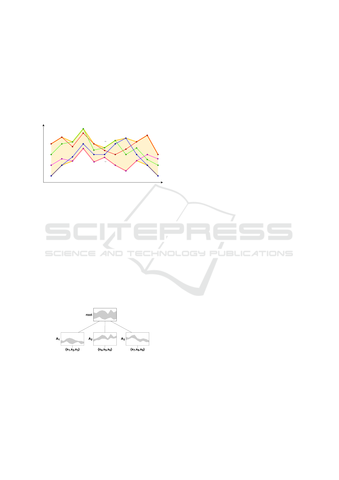
values at each time stamp (see Figure 1).

Figure 1: A set of four time series is enclosed by a “Mini-

mum Bounding Time Series” (MBTS) using the minimum

and maximum values at each time stamp. The result is a

pair of time series with upper B

⊓

and lower B

⊔

limit. Al-

though all time series are equally sampled in this example

illustration, this is not a requirement. Time series with dif-

ferent sampling can also be combined to form an MBTS.

As mentioned above, the TS-Index has a tree data

structure. Its internal nodes point to child nodes at

the next level. Each leaf node points to the starting

positions, relative to the input time series T , of its in-

dexed subsequences. All leaf nodes must be on the

same level. Furthermore, each internal node as well

as each leaf node has an MBTS that encloses all in-

dexed subsequences contained in the node. As the

number of indexed subsequences per node decreases

from the root node downwards, the MBTS also be-

come narrower.

Figure 2: The TS-Index is a tree structure with a pair of

boundary time series in each node.

The TS-Index construction requires an input time

series T and a desired subsequence length l. The in-

dex is constructed by sequentially extracting all pos-

sible subsequences of l length from T and inserting

them one by one into the TS-Index. As the construc-

tion follows a top-down approach, the tree must be

traversed from the root node to its leaf nodes when

inserting a subsequence S. At each level, the MBTS

of the nodes within are compared with S. By repeat-

edly selecting the nodes with the smallest distance to

S at each level, a leaf node is reached. Among all

leaf nodes, this leaf node has the smallest distance be-

tween its MBTS and S. Therefore, the starting posi-

tion of S can be added to the set to which this leaf node

points. As subsequences are added to the TS-Index,

a minimum-maximum criterion forces nodes to split

in order to evenly distribute the number of children

per node. The resulting tree structure is shown in Fig-

ure 2.

For a given query sequence Q, the twin subse-

quence search uses a ﬁlter-veriﬁcation algorithm. As

a prerequisite, the query sequence Q must be of the

same length as the subsequences used to construct the

TS-Index.

A subsequence S is similar to the query sequence

Q if the distance between the two sequences is less

than or equal to a desired threshold ε. Each node N

within the TS-Index contains an MBTS that bounds

all subsequences indexed by N. Thus, once the ﬁlter-

veriﬁcation algorithm encounters a node where the

distance between its MBTS and Q is greater than

ε, the search space can be pruned, as the algorithm

does not need to check for similar subsequences in

N and N’s child nodes. In this procedure, the algo-

rithm ﬁlters leaf nodes that contain possible twin sub-

sequences compared to Q. Then, in the veriﬁcation

phase, each subsequence S contained in the ﬁltered

leaf nodes is compared to Q.

3 METHOD

The extended method presented in this paper is based

on the TS-Index data structure introduced by Chatzi-

georgakidis et al. (Chatzigeorgakidis et al., 2021). It

extends the “Twin Subsequence Search in Time Se-

ries” approach in several ways:

• tree balancing for better performance,

• exploration method using self-similarities,

• not-a-number handling, and

• uncertainty quantiﬁcation.

3.1 Unbalanced Trees

The original implementation of TS-Index uses a

minimum-maximum criterion during the tree con-

struction to ensure an almost balanced tree for opti-

mal run-time performance. The tree is constructed by

Scale and Time Independent Clustering of Time Series Data

585

inserting one time series at a time. The maximum

capacity speciﬁes the limit when a node has to be

split into two new ones; the minimum capacity de-

ﬁnes the number of child nodes a parent node must

at least point to. When a node is split into two new

nodes, its indexed subsequences are assigned to one

of the two new nodes based on their similarity. The

main assumption of this approach is a common uni-

form distribution of all time series with a positive ex-

pectation value of the distance between two series. If

the distribution differs signiﬁcantly, especially if sev-

eral time series are the same, the advantages of the

tree structure for speeding up the search are no longer

effective and the disadvantages of the overhead of the

acceleration structure prevail.

Therefore, our implementation does not use a

minimum and maximum number of child nodes, but

the distance measure as a separation rule. Similar

(and especially identical) time series should be close

together in the tree structure, ideally in the same node;

very different time series should not be unnecessarily

grouped together. This is particularly useful if identi-

cal series occur frequently in the data.

3.2 Self-Similarities Between all Time

Series

Most data structures are optimized for a single search

task consisting of a query time series Q and a set T

of time series {T

, T

, . . . , T

}. The desired result is

the element T

with the smallest distances to Q – the

so-called nearest neighbour of Q in T .

In the context of exploratory time series analysis,

the task is similar, but differs in one important aspect:

the nearest neighbour query does not consist of a sin-

gle time series Q, which may not even be an element

of the set T , but of all elements {T

, T

, . . . , T

} of T .

This extended search for similar elements in a set in-

evitably leads to many “hits” – at least the number of

elements in T . When all elements of a set are com-

pared with all elements of the same set, these “hits”

occur on the diagonal:

. . . T

d(T

, T

) d(T

, T

) d(T

, T

)

d(T

, T

) d(T

, T

) d(T

, T

)

d(T

, T

) d(T

, T

) d(T

, T

)

These diagonal elements are usually not wanted in the

result list of similarities and can be easily ﬁltered out.

However, this problem does not only occur with

identical subsequences of the same time series, but

also with small temporal shifts in the start times of

two subsequences of the same sequence. The question

of whether these similarities are desirable in the list

of results cannot be answered without context. While

small temporal shifts should normally be ﬁltered out,

similarities with a large temporal offset indicate cycli-

cal, seasonal or generally recurring patterns within a

time series and are therefore desirable detection re-

sults. We have solved this problem with a new pa-

rameter ∆, which ﬁlters out self-similarities within

the same time series by means of a minimum time

distance threshold. This solution generalises the ﬁl-

tering to avoid the “diagonal self-similarity problem”

described above.

3.3 Not-A-Number

Apart from the theory, time series are characterised

by a multitude of potential problems: synchronisation

problems, calibration problems, sensor failures, etc.

Every real-world system therefore needs a strategy for

dealing with these problems.

Our approach contains three ﬁlters that require a

valid parameter range to be speciﬁed for each time

series: Values that are below this parameter range are

replaced by a user-deﬁned value; values that exceed

this parameter range are replaced by a second user-

deﬁned value; undeﬁned values (not-a-number) are

replaced by a third value.

The choice of these three replacement values

should be adapted to the metric used; in particular,

the error case of not-a-number propagation through

the calculation should be taken into account (Monni-

aux, 2008).

3.4 Uncertainty and Inaccuracy

Real data, even if complete, is always subject to mea-

surement error and imprecision (Fuller, 2006). This

imprecision should be represented together with the

data and also taken into account in the distance and

comparison metrics (Wang and Bi, 2021). By con-

sistently accounting for imprecision, a distance met-

ric on time series becomes a statistical adjustment

test (Zhang and Chen, 2018).

The approach we have chosen to cope with

imprecision and uncertainty extends a time series

, x

, . . . by quantifying uncertainty in terms of

standard deviations x

±t

, x

±t

, x

±t

, x

±t

, . . .

In the visualisation, this inaccuracy can be reﬂected

in a diffuse interval that is drawn semi-transparently

as an offset (Bhatt et al., 2021). Figure 3 shows the

visualisation of a time series including its standard de-

viations x

±t

IVAPP 2024 - 15th International Conference on Information Visualization Theory and Applications

586

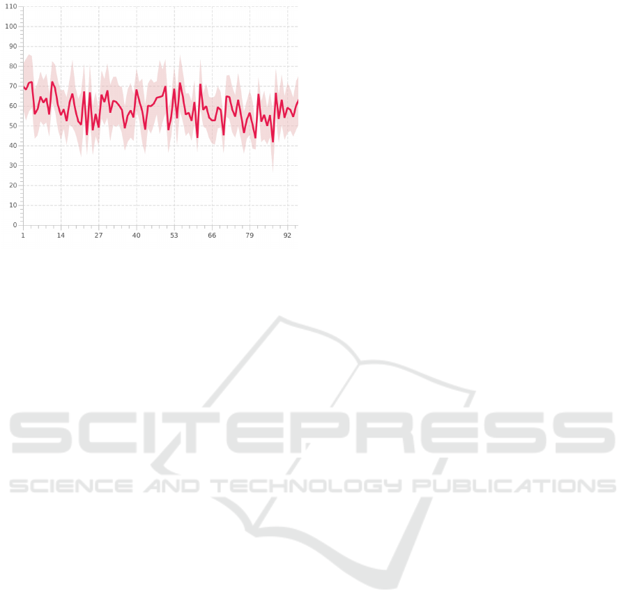
Figure 3: A time series of real data often contains measure-

ment errors and imprecisions. One method of communi-

cating these measurement errors and inaccuracies is to use

semi-transparent intervals surrounding a time series.

3.5 System Implementation

The TS-Index data structure and the ﬁlter veriﬁcation

search algorithms are implemented in Java. In addi-

tion, a graphical user interface (GUI) is developed us-

ing JavaFX to facilitate user interaction and provide

visualisations of the search results. The implementa-

tion of the system can be divided into two steps: the

construction phase and the clustering process.

In the construction phase, each time series is split

into all its possible subsequences using a sliding win-

dow. For each time series, a separate TS-Index is con-

structed by sequentially inserting the extracted subse-

quences. This approach is chosen over inserting all

subsequences into a single TS-Index due to the im-

proved efﬁciency it offers: This method allows us

to take advantage of multithreading, starting separate

threads for the creation of each time series’ TS-Index.

In contrast, inserting all subseries sequentially into a

single large TS-Index would lead to a higher num-

ber of node splits and distance calculations, resulting

in slower performance. The maximum node capacity

parameter is set to max = 5, which strikes a good bal-

ance between minimising the time required for node

splits and maximising the efﬁciency gained by early

search space pruning.

For the cluster creation, query sequences cover-

ing a speciﬁed time span are extracted from each time

series. The ﬁlter-veriﬁcation algorithm is then ap-

plied to each query sequence to search for similar

subsequences within the previously constructed TS-

Indices. Similar to the construction phase, the identi-

ﬁcation of similar subseries is performed concurrently

on separate threads for each query to further increase

efﬁciency. A threshold value is used to quickly decide

whether two time series are similar: The threshold is

set to the expected value of the absolute difference be-

tween two stochastically independent, uniformly dis-

tributed random variables X, Y . Distances greater

than this expected value E(|X −Y |) indicate a higher

probability of random occurrence, which means that

subsequences with such distances are not considered

to be twin subsequences of the query.

For each query sequence, the twin subsequences

identiﬁed by the ﬁlter veriﬁcation algorithm are fur-

ther sorted based on their Chebyshev distance to

the query. If the number of identiﬁed subsequences

exceeds the desired cluster size, the excess subse-

quences are removed. Notably, since the algorithm

compares the query to all time series indices, the

query sequence itself is included in the results due

to its distance of 0, thus ensuring its presence within

the cluster. Within a cluster, the subsequence with

the largest Chebyshev distance determines the over-

all cluster distance, allowing the clusters to be ranked

from most similar to least similar.

The GUI provides a visual interface for users to

interact with the system. Through the GUI, users can

select a metadata and time series attributes that will

display the corresponding time series in a line graph.

The graph provides information on observed values

and standard deviations. In addition, by hovering over

the time series, users can view different time series

values at the same time. To determine the time span

of queries for the clustering process, users can deﬁne

a speciﬁc start and end date of interest. The GUI al-

lows users to create clusters of a speciﬁed size con-

taining subsequences from all time series, or to per-

form a faster twin subsequence search for a speciﬁc

country and search term. The latter option also allows

users to specify a similarity threshold.

4 EVALUATION

The presented system is primarily used for the explo-

ration of one’s own time series and is adapted to the

speciﬁc needs and peculiarities of one’s own data.

4.1 Medical Data Analysis

The use case of the application is the data exploration

of several datasets, all based on the idea described in

“Detecting inﬂuenza epidemics using search engine

query data” (Ginsberg et al., 2009): people who no-

tice symptoms of an illness ﬁrst google for medical

advice before consulting a doctor. Thus, days before

an ofﬁcially conﬁrmed inﬂuenza epidemic (based on

Scale and Time Independent Clustering of Time Series Data

587

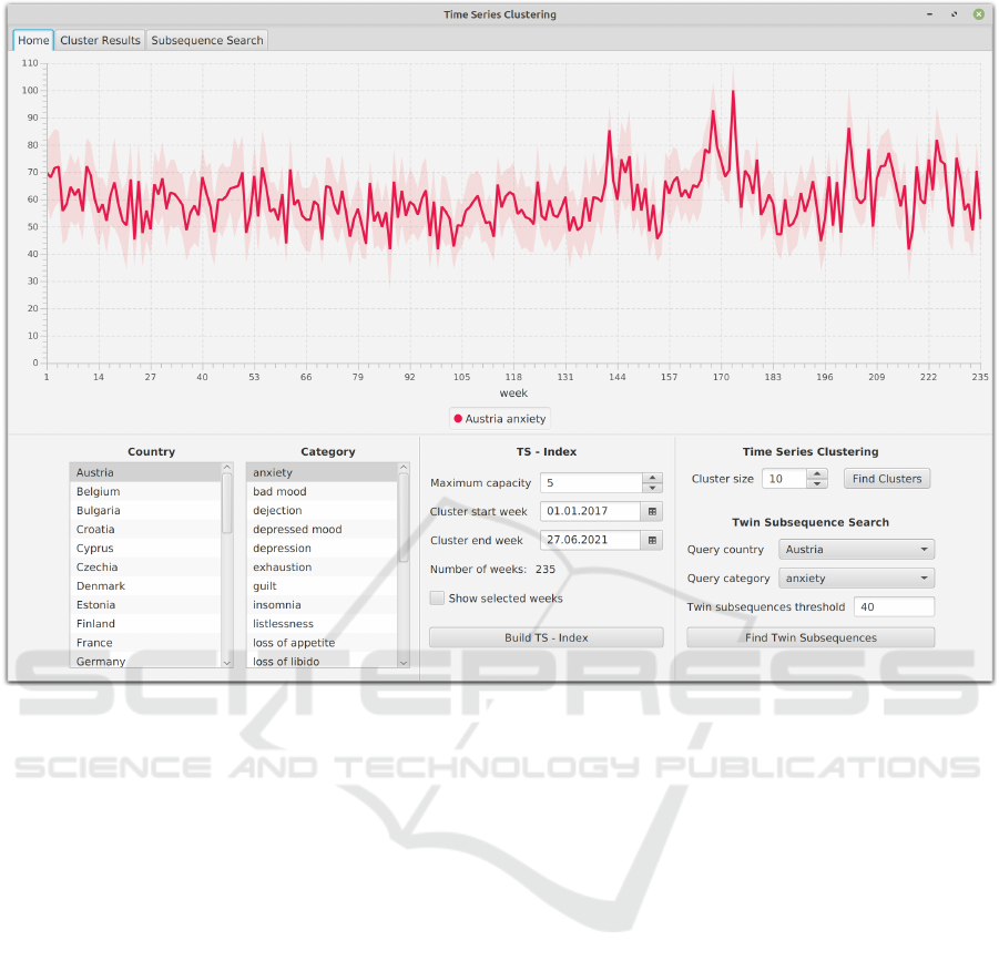
Figure 4: The ﬁrst visual inspection of the time series input data has the goal to check completeness and plausibility. Further-

more, this is the starting point of the interactive visual analytics process.

diagnoses with pathological test results), the Google

database already contains clusters of inﬂuenza-like

symptoms as search terms.

Following this idea, the COVID-19 pandemic has

been analysed. Each dataset contains a time series of

one country on a search term translated into the lo-

cal language and associated with a direct pandemic

symptom or an indirect health impact. The task of

exploratory data analysis is to look for similarities

and differences between countries and to relate these

to the number of cases and countermeasures (lock-

down, etc.) taken by each country. In detail, the

dataset consists of a list of countries. For each country

it comprises

1. a time series of COVID-19 cases reported to/by

the European Centre for Disease Prevention and

Control (ECDC),

2. a time series of COVID-19 counter measures (clo-

sure of ed. institutions, stay-at-home orders, . . . )

reported to/by ECDC,

3. a translated list of direct pandemic symptoms

(back pain, chest pain, . . . ) and indirect health

impacts (anxiety, depression, . . . ) into the of-

ﬁcial language(s) of the corresponding country

(based on the International Classiﬁcation of Dis-

eases, ICD-10), and

4. a time series of Internet query frequencies for

each entry of the translated list as reported by

Google Trends.

The starting point of the analysis is transformation

and normalisation of the individual time series (Keim

et al., 2008); Google Trends does not provide abso-

lute numbers of Internet queries, but only relative in-

creases and decreases. This step is completely auto-

matic; the starting point of the interactive visual anal-

ysis is the inspection of the data to visually check

its completeness and plausibility. Figure 4 shows the

graphical user interface (GUI) after loading and trans-

forming the dataset at the starting point of interactive

data exploration.

The visual analytics process aims to make the best

use of huge amounts of information in a wide range

of applications by combining the strengths of intelli-

gent automatic data analysis with the visual percep-

tion and analysis skills of the human user (Kohlham-

mer et al., 2011). This interactive process combines

data transformation, model building and model visu-

IVAPP 2024 - 15th International Conference on Information Visualization Theory and Applications

588

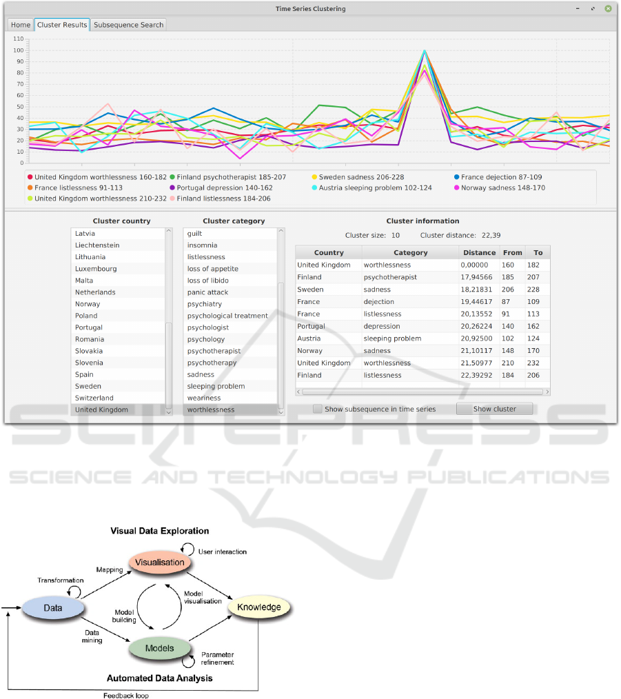
Figure 6: This screenshot shows a time series cluster centred on the time series “UK worthlessness 160–182”; the time series

describes the frequency of internet search queries from the UK containing the term worthlessness over the period from the

160th to the 182nd week since 1 January 2017.

alisation with the aim of gaining knowledge in an it-

erative loop (see Figure 5).

Figure 5: The visual analytics knowledge discovery process

combines data transformation, model building and model

visualisation in an iterative feedback loop (Keim et al.,

2010). Image source: (Kohlhammer et al., 2011).

In this particular application, the modelling and visu-

alisation is based on unsupervised clustering, which

identiﬁes the time series that are similar. The common

features found were then correlated with the context

(countermeasures) of the respective country to iden-

tify a general pattern. This pattern was then tested

for plausibility and further reﬁned by domain experts

from medicine and psychology. Figure 6 shows one

cluster of the clustering process applied to all time

series data. The similarity of the individual time se-

ries within this cluster to each other is particularly

striking from a visual point of view. This interac-

tive process resulted in common patterns identiﬁed in

the data; i.e., appropriate knowledge was extracted.

However, these ﬁndings need to be conﬁrmed. For

this purpose, the extracted hypotheses were analysed

with statistical tests and their signiﬁcance was eval-

uated. The medical and psychological ﬁndings are

published in “Google Trends for Pain Search Terms

in the World’s Most Populated Regions Before and

After the First Recorded COVID-19 Case: Infodemi-

ological Study” (Szilagyi et al., 2021) and “Impact

of the pandemic and its containment measures in Eu-

rope upon aspects of affective impairments: a Google

Trends informetrics study” (Szilagyi et al., 2023) and

are not the primary concern of this paper, which fo-

cuses on the process, the tools used in the process,

and the lessons learned.

Scale and Time Independent Clustering of Time Series Data

589

4.2 Filter Results & Effects

The ﬁrst step is to ﬁnd similar time series in the

frequencies of internet search queries from different

countries. The results are not always as nice as shown

in Figure 7.

Figure 7: Different keywords from searches in different

countries can show the same frequency over time.

However, some clusters from unsupervised cluster

analysis stand out from the rest, forming a subset of

time series that not only share similarities but also

a common problem. If there are not enough queries

from a country, Google Trends returns a correspond-

ing ﬂat line (complete or temporary). These zero

lines, indicating data gaps, are obviously similar to

each other and are therefore grouped into a cluster

(see Figure 8). Identifying these clusters and exclud-

ing them from further analysis reduces the subsequent

analysis effort and is therefore desirable.

Figure 8: Different keywords from searches in different

countries can show the same frequency over time.

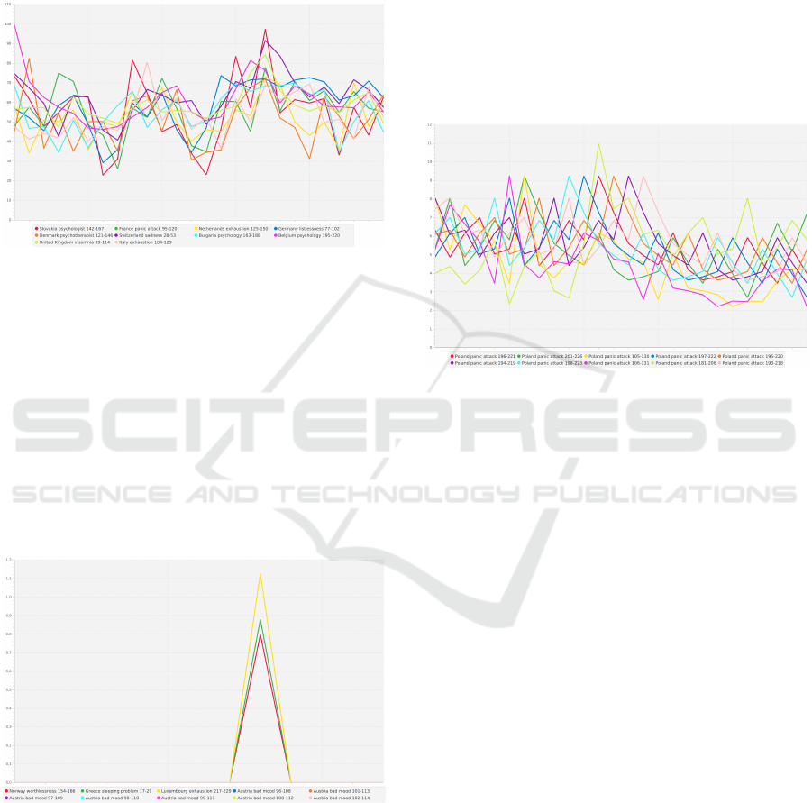
An undesirable similarity is self-similarity. Figure 9

illustrates such a situation: the Figure shows the fre-

quency distribution of the time series “Poland, panic

attack, 196–221”, i.e. the frequencies of search

queries from Poland containing the keyword “panic

attack” in the weeks 196 to 221 since 1.1.2017. This

time series is of course similar to the time series

“Poland, panic attack, 194–219”, which is only offset

by two weeks. Likewise, the cluster contains not only

the time series that was two weeks earlier, but also the

time series that was two weeks later and other variants

with different time offsets.

This self-similarity is in the nature of time series.

Any time series that is Lipschitz continuous has a

bounded distance to a time-shifted instance of itself.

This fact does not provide any new insight into the

application domain of time series and is therefore not

desirable.

Figure 9: Most time series are similar to shifted versions of

themselves. This fact provides no insight into the applied

use case.

However, this “uninteresting” self-similarity should

be excluded with caution in further analysis, as it be-

comes more “interesting” as the time shift increases.

Figure 10 shows one such interesting shift, which

prompted further investigation: Internet searches for

sleep problems in the United Kingdom show an an-

nual pattern. The corresponding time series with a

high level of similarity

• “United Kingdom, insomnia, 39–60”

• “United Kingdom, insomnia, 91–112”

• “United Kingdom, insomnia, 143–164”

are shifted by exactly 52 weeks. This annual peak

is a regularity that stimulates further analysis and re-

search (outside of time series analysis and partly out-

side of medical or psychological domains of appli-

cation). For this reason, the choice of the minimum

distance between two instances of a time series that

are shifted in time is critical and should not be made

carelessly.

IVAPP 2024 - 15th International Conference on Information Visualization Theory and Applications

590

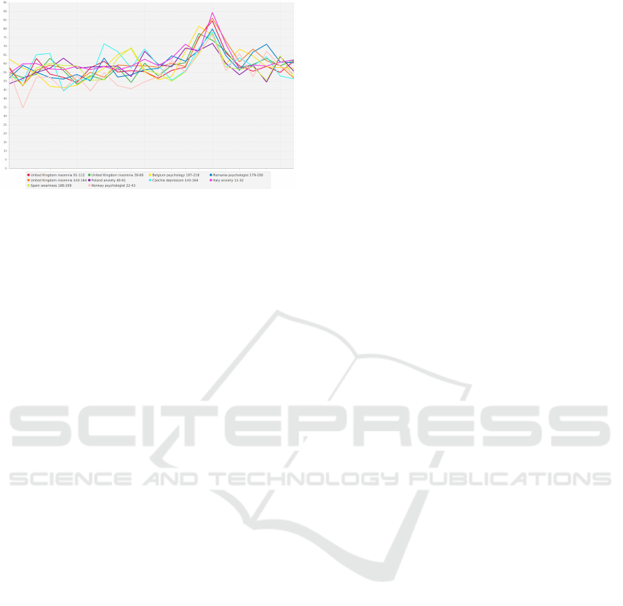
Figure 10: Seasonal and cyclical effects are self-similar.

Detecting these properties within time series can provide

new insights.

5 CONCLUSION

The presented time series analysis extends the state of

the art by several improvements that have been imple-

mented and tested on real data.

5.1 Contribution

Our contribution to the scientiﬁc community is the ex-

tension of the TS-Index approach to unbalanced trees

in order to prioritise similarity over performance op-

timised tree structures – especially in visual analytics

use cases with many similar elements, the similarity-

based tree structure can be beneﬁcial to analysis per-

formance. Many identical elements can be quickly

excluded when searching the tree.

The issue of self-similarity is also the subject

of our second suggestion for improvement: self-

similarity may be inherent in the time series or an

indication of an external, application-speciﬁc factor.

The detection of self-similarity is therefore both de-

sirable and unnecessary noise in the analysis. The

difference between the two possibilities is reﬂected in

the time difference: the shorter the shift between two

similar time series, the less interesting the similarity;

large distances, on the other hand, indicate interesting

patterns, especially seasonal or cyclical patterns. Ap-

propriate ﬁlters, such as those we have implemented,

offer the possibility of separation.

In addition to ﬁltering out unwanted self-

similarities, the efﬁcient and effective handling of

data problems (gaps, outliers, etc.) is a tedious but

important issue. In theory, these cases are consid-

ered much less often than in practice. Here we have

extended the existing algorithms with Not-a-Number

and Out-Of-Range mapping ﬁlters. These allow to

use of even short subsequences of valid time series

and not to ﬁlter or discard them. Furthermore, the

subsequent analysis steps do not need to consider spe-

cial cases (NaN, PosInf, . . . ).

We have also added imprecision and uncertainty

handling to the existing algorithms. Many time se-

ries (measurements, surveys, etc.) have precision in-

formation (range of variation, measurement precision,

etc.) that usually goes unnoticed. In our implementa-

tion, this is taken into account throughout and is also

displayed in the visualisations, if wanted.

5.2 Beneﬁt

The lessons learned from this study are particularly

valuable because the effects described are indepen-

dent of the application domain and can occur in many

different contexts.

The examples and the effects that occurred illus-

trate the problem of self-similarity and its ambiguous

nature: self-similarities due to short shifts should be

interpreted and ﬁltered as noise; with increasing tem-

poral distance, self-similarity gains importance and

should be taken into account.

Another important beneﬁt is the realisation that

cluster analysis can also be used for data inspection

and data transformation: similar errors often produce

similar indications, an example of the feedback loop

from knowledge back into data preparation.

ACKNOWLEDGMENT

The work was partially funded by the Austrian Re-

search Promotion Agency (FFG) within the frame-

work of the ﬂagship project ICT of the Future

PRESENT, grant FO999899544.

REFERENCES

Aghabozorgi, S., Shirkhorshidi, A. S., and Wah, T. Y.

(2015). Time-series clustering – A decade review. In-

formation Systems, 53:16–38.

Bhatt, U., Antor

an, J., Zhang, Y., Liao, Q. V., Sattigeri, P.,

Fogliato, R., Melanc¸on, G., Krishnan, R., Stanley, J.,

Tickoo, O., Nachman, L., Chunara, R., Srikumar, M.,

Weller, A., and Xiang, A. (2021). Uncertainty as a

Form of Transparency: Measuring, Communicating,

and Using Uncertainty. AAAI/ACM Conference on AI,

Ethics, and Society, 4:401–413.

Chatzigeorgakidis, G., Skoutas, D., Patroumpas, K., Pal-

panas, T., Athanasiou, S., and Skiadopoulos, S.

(2021). Twin Subsequence Search in Time Series. In-

ternational Conference on Extending Database Tech-

nology (EDBT), 24:475–480.

Scale and Time Independent Clustering of Time Series Data

591

Fuller, W. A. (2006). Measurement Error Models. Wiley-

Interscience, 1 edition.

Ginsberg, J., Mohebbi, M. H., Patel, R. S., Brammer, L.,

Smolinski, M. S., and Brilliant, L. (2009). Detecting

Inﬂuenza Epidemics using Search Engine Query Data.

Nature, 457:1012–1014.

Goldin, D. and Kanellakis, P. (1995). On similarity queries

for time-series data: Constraint speciﬁcation and im-

plementation. International Conference on Principles

and Practice of Constraint Programming, 976:137–

153.

Hennig, C., Meila, M., Murtagh, F., and Rocci, R.

(2015). Handbook of Cluster Analysis. Chapman and

Hall/CRC, 1 edition.

Hochheiser, H. and Shneiderman, B. (2003). Interactive Ex-

ploration of Time Series Data. The Craft of Informa-

tion Visualization, 1:313–315.

Keim, D., Andrienko, G., Fekete, J.-D., G

org, C., Kohlham-

mer, J., and Melanc¸on, G. (2008). Visual Analyt-

ics: Deﬁnition, Process, and Challenges. Information

Visualization (Lecture Notes in Computer Science),

4950:154–175.

Keim, D., Kohlhammer, J., Ellis, G., and Mansmann, F.

(2010). Mastering the Information Age Solving Prob-

lems with Visual Analytics. CEurographics Associa-

tion, 1 edition.

Keogh, E., Chakrabarti, K., Michael, P., and Mehrotra, S.

(2001). Dimensionality Reduction for Fast Similarity

Search in Large Time Series Databases. Knowledge

and Information Systems, 3:263–286.

Kohlhammer, J., Keim, D., Pohl, M., Santucci, G., and An-

drienko, G. (2011). Solving Problems with Visual An-

alytics. Procedia Computer Science, 7:117–120.

Monniaux, D. (2008). The pitfalls of verifying ﬂoating-

point computations. ACM Transactions on Program-

ming Languages and Systems, 30:1–41.

Neamtu, R., Ahsan, R., Rundensteiner, E., and Sarkozy, G.

(2016). Interactive Time Series Exploration Powered

by the Marriage of Similarity Distances. Very Large

Data Base (VLDB) Endowment, 10:169–180.

Ott, R. L. and Longnecker, M. T. (2015). An Introduction

to Statistical Methods and Data Analysis. Cengage

Learning, 7 edition.

Shieh, J. and Keogh, E. (2008). ISAX: Indexing and Mining

Terabyte Sized Time Series. International Conference

on Knowledge Discovery and Data Mining, 14:623–

631.

Szilagyi, I. S., Eggeling, E., Bornemann-Cimenti, H., and

Ullrich, T. (2023). Impact of the pandemic and its con-

tainment measures in Europe upon aspects of affec-

tive impairments: a Google Trends informetrics study.

Psychological Medicine, online:1–13.

Szilagyi, I. S., Ullrich, T., Lang-Illievich, K., Klivinyi,

C., Schittek, G. A., Simonis, H., and Bornemann-

Cimenti, H. (2021). Google Trends for Pain Search

Terms in the World’s Most Populated Regions Be-

fore and After the First Recorded COVID-19 Case:

Infodemiological Study. Journal of Medical Internet

Research, 23:e27214.

Wang, W. and Bi, L. (2021). Research on strategies to im-

prove model accuracy based on incomplete time series

data. Asian Conference on Artiﬁcial Intelligence Tech-

nology (ACAIT), 5:45–52.

Wu, J., Wang, P., Pan, N., Wang, C., Wang, W., and Wang,

J. (2019). KV-Match: A Subsequence Matching Ap-

proach Supporting Normalization and Time Warping.

IEEE International Conference on Data Engineering

(ICDE), 35:866–877.

Zhang, B. and Chen, R. (2018). Nonlinear Time Series

Clustering Based on Kolmogorov-Smirnov 2D Statis-

tic. Journal of Classiﬁcation, 35:394–421.

IVAPP 2024 - 15th International Conference on Information Visualization Theory and Applications

592