Semantic and Horizon-Based Feature Matching for Optimal Deep Visual

Place Recognition in Waterborne Domains

Luke Thomas

, Matt Roach

1 a

, Alma Rahat

1 b

, Austin Capsey

and Mike Edwards

1 c

Swansea University, Swansea, U.K.

UK Hydrographics Ofﬁce, Taunton, Somerset, U.K.

Keywords:

Place Recognition, Waterborne Imagery, Region Proposal, Image Segmentation, Unsupervised Learning.

Abstract:

To tackle speciﬁc challenges of place recognition in the shoreline image domain, we develop a novel Deep

Visual Place Recognition pipeline minimizing redundant feature extraction and maximizing salient feature

extraction by exploiting the shoreline horizon. Optimizing for model performance and scalability, we present

Semantic and Horizon-Based Matching for Visual Place Recognition (SHM-VPR). Our approach is motivated

by the unique nature of waterborne imagery, namely the tendency for salient land features to make up a

minority of the overall image, with the rest being disposable sea and sky regions. We initially attempt to

exploit this via unsupervised region proposal, but we later propose a horizon-based approach that provides

improved performance. We provide objective results on both a novel in-house shoreline dataset and the already

established Symphony Lake dataset, with SHM-VPR providing state-of-the-art results on the former.

1 INTRODUCTION

Waterborne imagery is an emerging domain within

computer vision, recent works include surveys on col-

lision avoidance (Zhang et al., 2021) in order to pre-

vent the loss and damage of autonomous vessels as

well as fully automated navigation proposals using

deep learning techniques (Yan et al., 2019; Xue et al.,

2019a; Xue et al., 2019b).

Visual place recognition (VPR) is a computer

vision task based on extracting features from geo-

labelled imagery and learning a good representation

to perform image retrieval. In other words, given a

query image of some location, we would like to re-

trieve an image of the same location so that an end

user can ﬁnd where they are. For land imagery, bench-

mark datasets for VPR are numerous due to a large

demand for AI autonomous car system training, how-

ever datasets for autonomous vessels are rare due to

the area being more niche.

Waterborne image sets do exist, such as

MaSTr1325 (Bovcon et al., 2019) for pixel-wise la-

belling tasks and the Singapore Maritime Dataset for

object detection (Moosbauer et al., 2019). However,

those designed for VPR speciﬁcally are mostly lim-

https://orcid.org/0000-0002-1486-5537

https://orcid.org/0000-0002-5023-1371

https://orcid.org/0000-0003-3367-969X

ited to inland water regions such as rivers and lakes

(Grifﬁth et al., 2017; Steccanella et al., 2020).

In this work we present a number of experi-

ments with the Semantic and Spatial Matching Visual

Place Recognition (SSM-VPR) pipeline (Camara and

reu

cil, 2019) that attempt to maximise performance

on an in-house shoreline imagery dataset covering the

area of the Plymouth Sound, UK. We modify SSM-

VPR a number of times and apply each version to this

dataset as well as the Symphony Lake dataset (Grif-

ﬁth et al., 2017) to facilitate a comparison between

shoreline and inland water-based imagery.

We modify SSM-VPR in a number of ways, ﬁnd-

ing that the most effective modiﬁcation of the pipeline

for dealing with shoreline imagery is to encourage

structural consistency of features along the visible

horizon between a query and retrieval, creating a

novel pipeline that we dub Semantic and Horizon

Based Matching Visual Place Recognition (SHM-

VPR).

Before SHM-VPR, we theorised that unsuper-

vised region proposal could mimic real world naviga-

tion techniques, where landmark identiﬁcation is pre-

ferred over a more computer-like brute force search.

We experimented with two separate unsupervised re-

gion proposal methods, Selective Search (Uijlings

et al., 2013) and a unique method proposed in the

rOSD paper (Vo et al., 2020).

Thomas, L., Roach, M., Rahat, A., Capsey, A. and Edwards, M.

Semantic and Horizon-Based Feature Matching for Optimal Deep Visual Place Recognition in Waterborne Domains.

DOI: 10.5220/0012376000003654

Paper published under CC license (CC BY-NC-ND 4.0)

In Proceedings of the 13th International Conference on Pattern Recognition Applications and Methods (ICPRAM 2024), pages 761-770

ISBN: 978-989-758-684-2; ISSN: 2184-4313

761

A key part of our novel pipeline is the use of the

WaSR segmenter (Bovcon and Kristan, 2021) to clas-

sify which pixels represent land, sea and sky. As we

will see later, WaSR also allows us to identify feature

devoid images containing no land information, which

are typically not retrieved successfully as there are no

useful locational features visible. These images un-

fairly offset metrics such Precision-Recall Curves and

makes performance difﬁcult to gauge. Using WaSR

to calculate how many pixels in each image repre-

sent land lets us ﬁlter out feature devoid images via a

threshold, giving a clearer reﬂection of actual model

performance.

Ultimately, we ﬁnd our SHM-VPR pipeline to

provide state of the art results on our in-house shore-

line image dataset, although we note that it is a

domain-speciﬁc pipeline, and does not translate to in-

land locational imagery. SHM-VPR works by using

the pixel-wise labellings from WaSR to extract an ap-

proximated horizon line by ﬁnding the y position of

the ﬁrst land labelled pixel in each column of the im-

age, then projecting these coordinates onto a feature

map. The projected horizon line is then used to guide

a sliding window by keeping it centred on the y coor-

dinates as it moves along the x axis, extracting a row

of structural vectors along the horizon.

2 RELATED WORK

2.1 Finding Salient Information in

Shoreline Imagery

In Visual Place Recognition, detecting notable land-

marks is an integral part of early handcrafted meth-

ods. For example, Scale Invariant Feature Trans-

form (SIFT) (Lowe, 1999) focuses on the identiﬁca-

tion of invariant key points which are then used to

form descriptors. With land imagery, notable land-

marks come in a variety of forms and can be located

at various different positions in an image. However

we ﬁnd that shoreline imagery lacks these traditional

conspicuous landmark structures.

In the majority of shoreline images, the top and

bottom halves are made up mostly of sky and sea re-

spectively, both of which are largely redundant for

place recognition as they have no inherently notable

features. Having the sky be so prominent in an im-

age also introduces unwanted variation depending on

time, weather conditions and cloud formations. Land

images suffer less from this as the sea and sky are

normally both less prominent. Furthermore weather

conditions such as fog more negatively impact shore-

line imagery since distant land become almost totally

concealed.

Increasing distance between the capture camera

and shore compounds these issues, as the shoreline

itself will appear progressively smaller, taking up a

smaller percentage of the image. This also intro-

duces a hardware limitation, where only high reso-

lution cameras are still capable of capturing detailed

shoreline features. When traditional landmark fea-

tures such as buildings are no longer captured in de-

tail, relying on general topology becomes more nec-

essary.

Sky and sea sections impacting activation maps

can be remedied by using a segmentation model such

as WaSR (Bovcon and Kristan, 2021) to mask out

these areas before making a forward pass on an im-

age, however this leaves the images with a lot of blank

space. We could crop the image down to the land area

but to still get standardized feature maps they would

need to be resized, distorting visible topology. Errors

in the prediction mask could also offset the crop in

cases where there are pixels above or below the shore

erroneously identiﬁed as land.

The overall challenge here is to ﬁrst identify

which part of the image contains land features and,

secondly, to make sure the pipeline is extracting as

much feature rich information from this subset as pos-

sible.

2.2 SSM-VPR: Semantic and Spatial

Matching Visual Place Recognition

The pipeline we have chosen to focus our study

around is SSM-VPR, a two stage pipeline pub-

lished by Camara and Preucil in 2019 (Camara and

reu

cil, 2019). SSM-VPR uses the VGG16 net-

work (Simonyan and Zisserman, 2014) pre-trained on

Places205 (Zhou et al., 2014) as a backbone for gener-

ating feature maps that are then divided into localized

sub-regions and vectorized in a two stage approach.

Stage 1 applies a sliding window to designate a set

of sub-regions, these are then vectorized and added to

the Image Filtering Database (IFDB), storing multi-

ple vectors per image in this way makes the model ro-

bust to viewpoint changes because as previous works

have discovered, using multiple region vectors boosts

performance for visual place recognition (S

underhauf

et al., 2015; Chen et al., 2017b; Khaliq et al., 2019).

Stage 2 performs a similar procedure with a

smaller sliding window, designating a new set of

many ﬁne sub-regions containing structural details

from the feature map. These are then vectorized and

added to the Spatial Matching Database (SMDB).

Once the IFDB and SMDB are built the pipeline

can then be passed a query image which it extracts

ICPRAM 2024 - 13th International Conference on Pattern Recognition Applications and Methods

762

the same two sets of vectors from. Stage 1 query vec-

tors are matched one by one to a set of nearest neigh-

bours in the IFDB, images associated with these re-

ceive points on a histogram. The top N scores then

make up the initial retrieval images.

Stage 2 acts as a re-ranking stage (Tolias et al.,

2015) where query and retrieval image SMDB vectors

are spatially re-arranged into the order they were pre-

viously extracted via sliding window. Spatial Match-

ing is then performed, identifying anchor points be-

tween the query and each individual retrieval. For

each anchor point we check the surrounding vectors

and each time a pair of vectors at the same location

relative to their anchor points are found to be a clos-

est match, the retrieval receives a point on a new his-

togram which is used for re-ranking.

SSM-VPR outperforms several state-of-the-art vi-

sual place recognition models on ﬁve benchmark

datasets (Camara and P

reu

cil, 2019). It has also had a

follow-up paper, where a frame correlation technique

was built in to further improve performance by pro-

moting retrievals that are consistent with previously

identiﬁed locations (Camara et al., 2020).

2.3 WaSR: Water Segmentation and

Reﬁnement

WaSR is an obstacle detection network intended for

use on small Unmanned Surface Vehicles (USV)

which instead of using expensive heavyweight range

sensors such as RADAR, LIDAR or SONAR

(Onunka and Bright, 2010; Ruiz and Granja, 2009;

Heidarsson and Sukhatme, 2011) seek to use com-

puter vision enabled on-board cameras to minimize

cost and weight (Kristan et al., 2015).

For our work we are only concerned with utilis-

ing WaSR’s segmentation capabilities, which uses a

novel encoder-decoder architecture, with the encoder

generating deep features that are fused with the de-

coder, with an optional Inertial Measurement Unit

(IMU) feature channel used to aid in the detection of

the water-edge (Bovcon et al., 2018).

The IMU measurement encoder allows the model

to use encoded inertial data to project the horizon onto

the image itself to aid in detecting the precise water

edge, which is particularly challenging for a convolu-

tional encoder to detect alone as camera haze induced

by weather conditions or water obstructing the cam-

era blurs feature maps around the true water edge.

The encoder is based on the segmentation back-

bone from DeepLab (Chen et al., 2017a) which ap-

plies atrous convolutions to ResNet101. The encoder

uses the output of residual blocks 2, 3, 4 and 5 to

leverage both the generalized, low resolution features

from the later blocks with the more ﬁne high resolu-

tion information of the earlier blocks. These features

are then passed to the decoder where they are fused

with information from the IMU encoder in order to

reﬁne the ﬁnal segmentation.

2.4 Region Proposal Methods

Region Proposal is a subset of object detection, where

the task is to try and identify which areas of an im-

age contain object-like features. The ﬁrst of these

methods were algorithms such as Selective Search

(Uijlings et al., 2013), but recently end-to-end train-

able Region Proposal Networks (RPN) such as Faster-

RCNN (Ren et al., 2015) have been developed, which

use fully-convolutional networks to predict object

bounds and per-pixel objectness scores.

Region Proposal Nets can achieve state of the art

results on region proposal tasks, however this requires

a dedicated image set with ground truth object labels

and bounding boxes to facilitate training. For land im-

agery this is not an issue as their are many open source

Region Proposal Nets pre-trained on datasets such as

ImageNet (Deng et al., 2009). However, because we

are dealing with shoreline imagery whose common

features are drastically different to the kinds found in

ImageNet, these pre-trained nets do not translate to

our data.

Designing new ground truth bounding boxes and

class labels for this new domain would be an incredi-

bly time consuming task and would likely require in-

sight from expert skippers or geographers. As com-

puter vision researchers, our knowledge on shoreline

geography and which land formations would count as

independent classes is also limited.

Therefore we opt to use unsupervised region pro-

posal algorithms, as these methods have some po-

tential to translate over to our domain by pointing

out unique geographical features. It also provides

an interesting opportunity to analyse what features

these algorithms identify as object-like when pre-

sented with this new domain.

Being the most common method, Selective Search

is an obvious retrieval, combining typical exhaustive

search with segmentation. Initially a given image is

sub-segmented into various small regions and from

then on the program begins a loop of taking two sim-

ilar regions from the set and combining them into a

larger region until we get a ﬁnal set of individual seg-

mentations, whose vertical and horizontal bounds are

used to make bounding boxes.

Selective Search can be computationally expen-

sive for large images queries, one of the driving forces

for the development of Fast R-CNN (Girshick, 2015),

Semantic and Horizon-Based Feature Matching for Optimal Deep Visual Place Recognition in Waterborne Domains

763

which instead projects region proposals from a larger

image onto it’s CNN feature maps and Faster R-CNN

(Ren et al., 2015), which uses it’s RPN to propose re-

gions based on the feature map itself, and, because

feature maps are dimensionally much smaller, this re-

sults in a faster computation. Selective Search itself

can also be applied on feature maps directly, however

it is not trained to work with such smaller dimensional

data in the way that Faster R-CNN is.

There have been newer algorithms for region pro-

posals since selective search was made, such as in Vo

et al’s (Vo et al., 2020) work, where in the process of

building upon the object and structure and discovery

problem (OSD) the authors presented their own re-

gion proposal algorithm. The algorithm in question is

based on the idea that, when summed along the ﬁlter

axis, CNN feature maps act as a single channel im-

age where objects from the original are represented

as clusters of high activations.

This method ﬁnds a set of local maxima within a

summed feature map using persistence measurement

(Chazal et al., 2013), and for each maxima a new fea-

ture map is generated by creating a dot product be-

tween the original CNN feature map and the feature

vector at the position of the maxima. The feature map

produced from this dot product is then summed along

the ﬁlter axis much like before to get a new image,

where the connected components algorithm is then

applied with a bounding box around the component

being the proposed region.

3 METHODOLOGY

3.1 Datasets

3.1.1 Symphony Lake

To measure performance on an existing dataset, we

use the Symphony Lake image set (Grifﬁth et al.,

2017), which covers a single lake in Metz, France, a

relatively compact inland area. The autonomous ves-

sel used for capture traverses along the lake edge so

not a great distance from shore, as such the dataset is

not a huge departure from typical land imagery. It is

comprised of various individual runs around the lake

between 2014 and 2017, providing coverage of the lo-

cations under different weathers, times and seasons.

For evaluation we use leave-one-out cross valida-

tion with seven randomly chosen image set runs, so

that the model can be evaluated on several unseen runs

while avoiding too much information from previous

runs leaking into the retrieval set.

3.1.2 Plymouth Sound Dataset

Our in-house dataset covers an area of the South

Coast of England, UK. The image set consists of 7

runs within this area between March and April 2022,

beginning from Turnchapel Wharf and taking var-

ious different routes within the area before return-

ing. Images were captured from on-board mounted

cameras attached to the IBM/Promare Mayﬂower Au-

tonomous Ship.

The dataset mostly consists of images taken far

from nearby shores, as well as some taken much

closer to shore as the vessel proceeded to embark

and disembark on each run. This makes the image

set unique as locational features are typically more

sparse and far away from the camera, meaning fea-

ture visibility can change drastically depending on

weather conditions, furthermore redundant informa-

tion (i.e Sea and Sky) is ever-present, with statistics

from WaSR segmentations suggesting that on average

only 5% of pixels in the image set are “land”, however

this statistic is greatly inﬂuenced by the large number

of images of open sea.

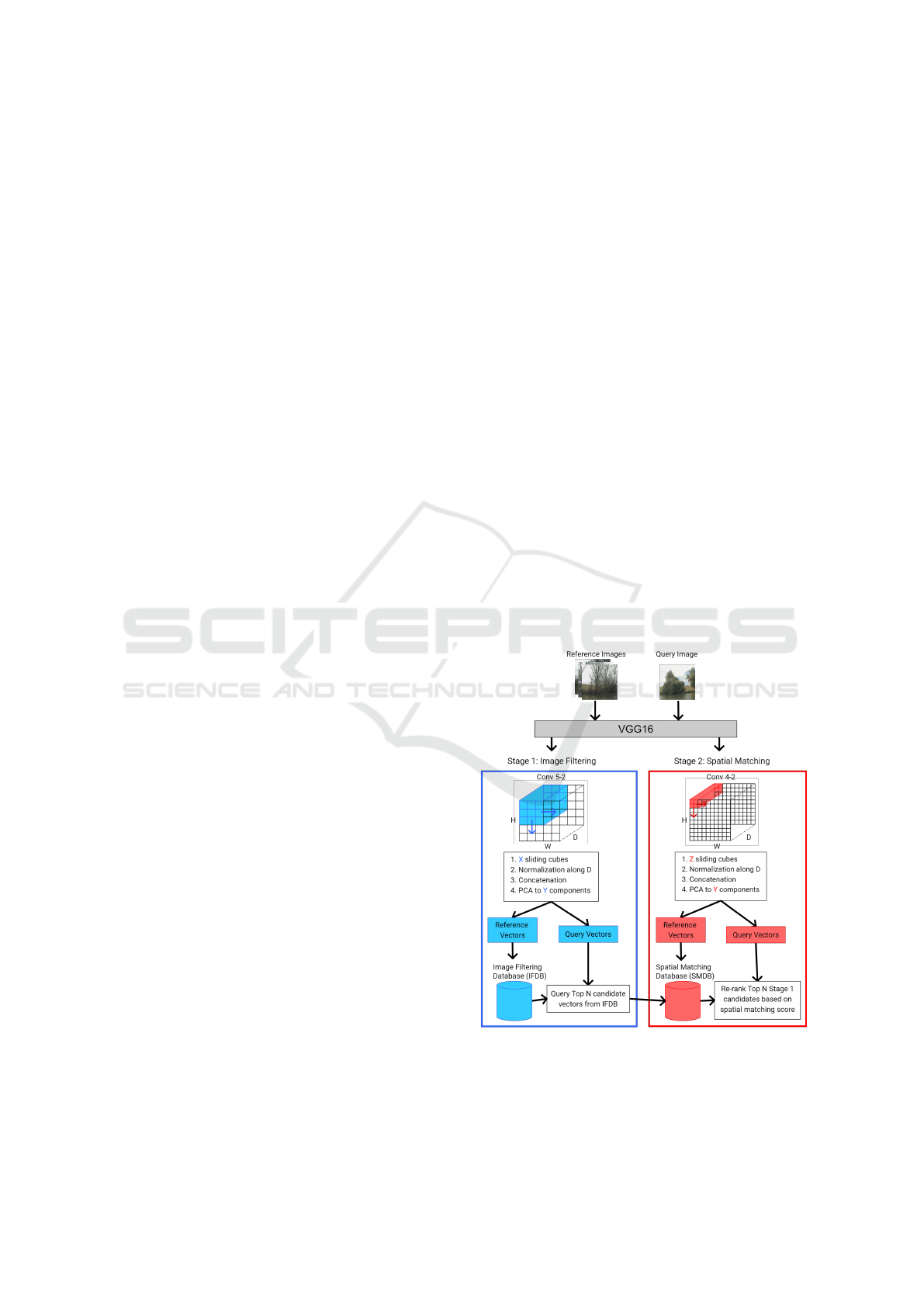
3.2 Pipelines

3.2.1 Base SSM-VPR

Figure 1: The pipeline of Base SSM-VPR, as described in

(Camara and P

reu

cil, 2019).

Depicted in Figure 1 is the original SSM-VPR

pipeline, for stage 1 we use the suggested resolution

ICPRAM 2024 - 13th International Conference on Pattern Recognition Applications and Methods

764

of 224 × 224 for our images, producing a feature map

of 14 × 14 × 512 over which we use a sliding win-

dow of 9× 9 for sub-region extraction. Resolution for

stage 2 is 448 × 448, which was found to be more ef-

fective in the pipelines follow up paper (Camara et al.,

2020), resulting in a feature map of 56 × 56 × 512 di-

mensions, the sliding window applied to this map has

a dimension of 3 × 3.

We made one change concerning the extraction

of sub-regions in both stages, we noticed that be-

cause the VGG16 backbone uses same padding for

each convolutional layer the edges of each feature

map become highly activated, adding false edge fea-

tures to the search databases. Therefore we limit the

range of the sliding windows to avoid the edges of

the feature maps. All hyper parameters were based

on those deﬁned by the SSM-VPR code on Github

(https://github.com/Chicone/SSM-VPR/).

3.2.2 Selective Search Based SSM-VPR

This pipeline incorporates selective search into SSM-

VPR stage 1 as an alternative to sliding window. In-

put images are now scaled to the same resolution as

stage 2 in order to return a larger feature map from

which selective search can extract an adequate num-

ber of suggested regions from.

Once a feature map is returned, a copy is made and

summed along the ﬁlter axis to produce a 1-D image

for selective search, the top N regions are then fed to a

Region Of Interest (ROI) Pooling layer along with the

original feature map, producing a set of 9 × 9 × 512

pooled sub-regions. We chose to pool to this resolu-

tion to maintain consistency for stage 1 sub-regions

across pipeline versions.

3.2.3 rOSD Region Proposal Based SSM-VPR

This pipeline operates similarly to the previous, swap-

ping out selective search region proposal for the

method described in the rOSD paper (Vo et al., 2020).

Because it is recommended to take input feature maps

from multiple layers of VGG16, we pass input images

up to two different convolutional layers of VGG16,

Conv 5-3 and Conv 4-3 as suggested in (Vo et al.,

2020), resulting in two feature maps per input image.

Copies of the maps are made, summed along the

ﬁlter axis and have rOSD region proposal applied to

them, we take N/2 suggested regions from both to get

N overall suggestions.

These suggestions are then fed to an ROI Pooling

layer along with the Conv 5-3 output feature map as

input, once again giving us a set of 9× 9 × 512 pooled

sub-regions. All other hyper parameters and parts of

the pipeline remain unchanged.

3.2.4 Semantic and Horizon-Based Matching for

Visual Place Recognition

Figure 2: Our SHM-VPR pipeline, here SSM-VPR stage 1

is kept the same as baseline but stage 2 now uses an esti-

mated horizon line based on WaSR and projects it onto the

feature map, the sliding window then moves along the map

in a single row across the x-axis, using the y coordinate of

the projected horizon line at each step.

The last version is our proposed SHM-VPR model,

this model keeps stage 1 of SSM-VPR the same and

focuses on making edits to stage 2. This method is

dependent on the WaSR segmenter and leverages it’s

prediction mask to extract a set of coordinates that

represent the position of the horizon line in the image.

Using these coordinates, stage 2 applies a sliding

window that only moves across the x axis of the fea-

ture map once, with the y coordinate at each step be-

ing determined by projecting the horizon line onto the

feature map and getting a set of approximate coordi-

nates.

This leaves a single row of stage 2 sub-regions,

exponentially reducing the number of vectors in the

SMDB. The spatial matching stage, which checks

for closest neighbour consistency around spatially

arranged anchor vectors between a query and re-

trieval still works but now only needs to check clos-

est neighbours around these anchors in a single di-

mension rather than checking for closest neighbours

Semantic and Horizon-Based Feature Matching for Optimal Deep Visual Place Recognition in Waterborne Domains

765

in 2 dimensions using baseline SSM-VPR’s grid of

extracted vectors.

The motivation is that throughout testing the hori-

zon line was the most consistently activated feature.

Landmarks such as buildings only make up a small

portion of the image and at long distance have limited

resolution, producing few highly activated features,

so now the re-ranking stage is more focused on spa-

tially matching only the most visually apparent and

variable structure of the shoreline images.

4 EVALUATION

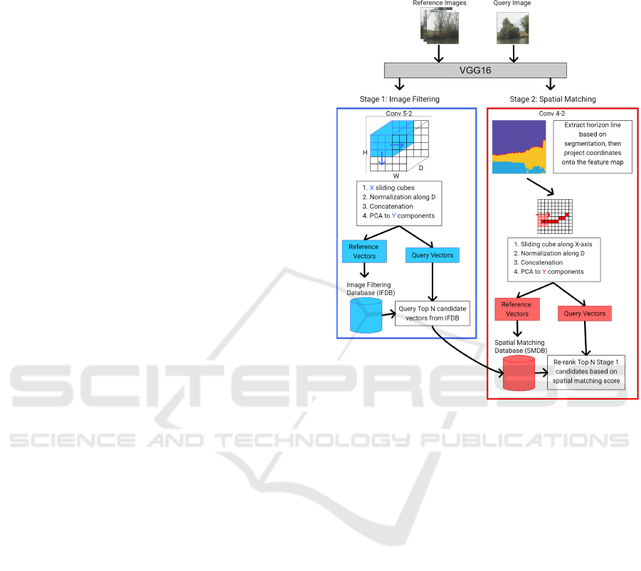
4.1 Quantitative Analysis

After collecting PR curves the seven test folds of both

datasets using base SSM-VPR, we can see from the

top plots in Figure 3 that results are consistently high

for Symphony Lake whereas there is a lot of varia-

tion in test folds for the Plymouth Sound dataset. To

explain this variance, a closer look is needed for the

imagery in the dataset.

Because the Plymouth Sound dataset was col-

lected using a multi-directional camera system we are

left with a signiﬁcant number of blank images con-

taining nothing but sky and sea. As expected, these

examples cannot be reasonably retrieved as they have

no useful data, and because they make up a signiﬁ-

cant percentage of each test fold, the effective maxi-

mum recall of each fold is limited. We alleviate this

by using statistics from the WaSR segmenter, calcu-

lating land, air and sea segmentations we get the av-

erage percentage of pixels in the image set that are

land which is around 5%, likely being inﬂuenced by

empty images. Using this number as a threshold for

what is an acceptable percentage of land pixels, we

ﬁlter out empty images and remove their inﬂuence to

get a better understanding of model performance.

After applying this threshold we get the bottom

plots in Figure 3, these curves are now more consis-

tent and are able to reach similar AUC values to the

Symphony Lake evaluations.

We will be utilizing this threshold for all PR curve

comparisons, to ensure evaluation is fair. We will also

be normalizing and averaging PR curves seen in Fig-

ure 3 into a single curve for each version of the SSM-

VPR pipeline for increased clarity.

Looking at PR curves, the selective search and

rOSD regions models perform worse than baseline

SSM-VPR on both datasets, for reasons we will dis-

cuss in our qualitative analysis it is clear that although

still functional, the ability of these pipelines to extract

meaningful sub-regions of various sizes as opposed to

the ﬁxed sub-regions of baseline falls short.

These methods add extra complexity and thus in-

ference time is slower on average, so unless we make

further edits in future, we deem unsupervised region

proposal integration into SSM-VPR to be unsuccess-

ful.

However our fourth pipeline, SHM-VPR, man-

ages to surpass SSM-VPR on Plymouth Sound but has

worse performance on Symphony Lake. This indi-

cates that our method is an improvement for our spe-

ciﬁc target domain of shoreline imagery but does not

translate as well to the more small-scale Symphony

Lake.

If we consider scalability however then there is an-

other advantage, to store all of the stage 1 and 2 vec-

tors for SSM-VPR each of our Plymouth Sound test

sets required around 18GB of storage space, most of

which is taken up by the stage 2 vector database due

to the sliding windows small size and the larger ex-

traction feature map of 56× 56 making for 54 × 54 =

4608 valid regions that must be stored as structural

matching vectors.

SHM-VPR only produces 54 vectors per image

for stage 2 because the sliding window does not per-

form an exhaustive search along the y axis for each

x axis coordinate, instead covering a single y coordi-

nate dictated by our approximated horizon line pro-

jection. This means SHM-VPR requires exponen-

tially less storage space for the structural matching

database and stage 2 is more streamlined.

4.2 Qualitative Analysis

Now that we’ve gone over the statistical performance

of each model, we carry out a secondary analysis

of the results by looking at visual representations of

what is happening when each pipeline is applied to

our shoreline imagery.

Figure 5 shows a set of true positives, viable query

images which the pipeline retrieved successfully, false

negatives, viable query images that were not retrieved

successfully and true negatives, unviable query im-

ages as determined by thresholding them based on

land pixel percentage based on segmentation results

from WaSR.

Looking at the true positive set, we see that most

images are those with clear shots of local coastline,

with recognizable shapes and minimal obstructions.

The false negative set contains some images erro-

neously labelled as valid due to interference from ob-

jects such as boats, which WaSR identiﬁes as land

thus boosting their land pixel percentage, this set also

contains some blurred/obstructed images as well as

more clear cut fail cases. The true negatives give a

ICPRAM 2024 - 13th International Conference on Pattern Recognition Applications and Methods

766

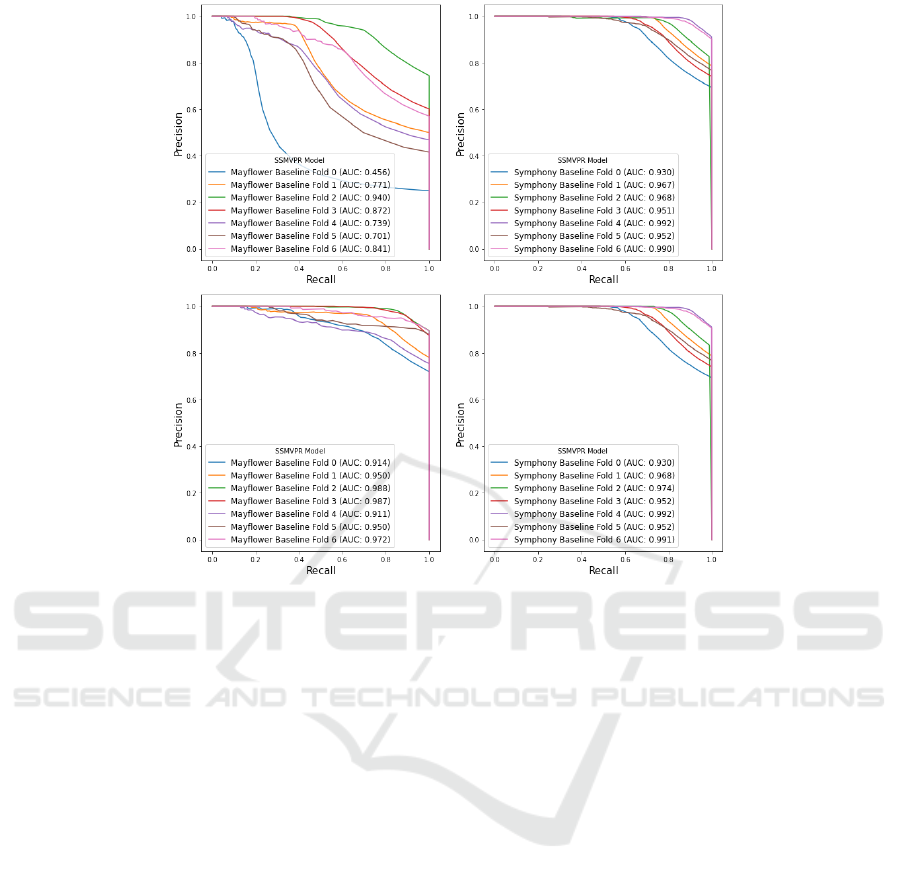
Figure 3: Top plots show PR curves on full dataset, across k-folds, containing samples with <5% land. Bottom plots show

PR curves on the same folds, omitting samples with <5% land after WaSR segmentation.

good example of feature devoid images, most of these

are either pointed out at sea where there is no land in-

formation, are severely lacking in shoreline features

or are so blurred due to water obstruction that WaSR

does not identify the present features as land.

This pattern is largely the same between model

variants, with each having slightly different true pos-

itive and false negative rates, reﬂected by the pre-

viously discussed PR Curves. To show how each

pipeline interacts with a given query image, we will

dedicate a section to how version 1, 2 and 3 of SSM-

VPR handles stage 1, and another section to show the

difference between the baseline stage 2 methodology,

which is consistent across the ﬁrst three versions, and

stage 2 of SHM-VPR.

4.2.1 Comparison of Different Approaches to

SSM-VPR Stage 1

Starting with a baseline model, given a query im-

age stage 1 of SSM-VPR takes the activation map

and divides it into a set of ﬁxed regions via sliding

cube. When visualised, we see that each region acts

as a slight perspective shift. When we match retrieval

vectors to each individual vectorized region and rank

them via histogram score based on the image ID as-

signed to each retrieval vector, we make sure that each

image retrieval must match the query across multi-

ple perspectives which incentivizes the return of a re-

trieved image that not only contains the same features

as the query, but also views them from a similar per-

spective and thus from a similar position.

For Selective Search based SSM-VPR, we receive

a number of suggested sub-regions which we then use

for SSM-VPR stage 1 region based vector extraction.

This means that instead of each sub-region represent-

ing a slight perspective shift of the overall image, each

one now represents an area of interest which in theory

should be similar to how mariners point out a series

of landmarks.

We know from the previous section that this

method does not perform as well as the baseline, the

reason for this could be seen in Figure 7, where the

selective search algorithm’s attention is often drawn

away from the land strip by areas of sea and sky.

There is also object interference, in the example a

boat appears in the image and remains visible in the

activation map. Objects like this draw attention from

the selective search algorithm, which is undesirable

for place recognition as it is a variant feature, the boat

could simply move or not be visible at any time if a

picture of the location were to be taken again, adding

Semantic and Horizon-Based Feature Matching for Optimal Deep Visual Place Recognition in Waterborne Domains

767

Figure 4: PR Curves for our four model versions on Plymouth Sound (Left) and Symphony Lake (Right), each averaged

across all test folds. Baseline model and Unsupervised Region Proposal variants are consistent across both sets, SHM-VPR

performs best on Plymouth Sound but the worst on Symphony Lake.

Figure 5: A set of True Positive (Top Row), False Negatives

(Middle Row) and True Negatives (Bottom Row) from a

single test fold of the baseline SSM-VPR pipeline.

Figure 6: Example of SSM-VPR semantic regions: For a

single image, the VGG16 activation map is summed along

the ﬁlter axis and set of sub-regions are extracted via sliding

window.

erroneous data to our vectors.

Overall it appears selective search is not able to

discern the types of sub-regions across the shore-

line, likely due to it being unsupervised and there-

fore not geared speciﬁcally to the shoreline image do-

main. In order to verify the effectiveness of incorpo-

rating unsupervised region proposals into SSM-VPR,

we tested a rOSD region proposal based SSM-VPR

pipeline, however results show this failed to compete

with baseline SSM-VPR.

Given an example of rOSD Region Proposal sug-

gestions on a feature map, we see that it actually man-

ages to single out the shoreline quite effectively, how-

ever the issue here is one of redundancy, most re-

gions are simply repeats of each other. This means

the number of unique sub-regions and perspectives of

Figure 7: Example of SSM-VPR with semantic regions

based on selective search: For this image, the activation is

summed along the ﬁlter axis, then selective search region

suggestions are made based on this and a set sub-regions

are extracted based on these.

Figure 8: Example of SSM-VPR with semantic regions

based on the rOSD paper region proposal method: Iden-

tical to Figure 7 only that the suggested regions are using

the rOSD method.

the shoreline is lower even though most notable areas

have been covered.

These examples also showcase that ROI pooling

these regions to maintain consistency may not be

ideal - many patches have seemingly lost their distinc-

tive shapes once pooled and reduced down to simple

edges.

4.2.2 Comparison of Different Approaches to

SSM-VPR Stage 2

As we have already discussed in the pipelines sec-

tion, SSM-VPR stage 2 forms a larger grid of much

ﬁner vectors for each image and for each retrieval re-

ranks them based on the number of spatial consistency

matches across a set of anchor vectors.

This method is very effective for re-ranking as it

ensures the top retrieval is highly spatially equivalent

with the query, making it more likely that the im-

ICPRAM 2024 - 13th International Conference on Pattern Recognition Applications and Methods

768

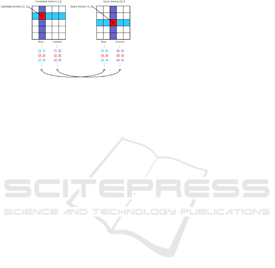
Figure 9: Figure inspired by the original paper (Camara and

reu

cil, 2019). A simpliﬁed representation of the spatial

matching stage for a grid of query and retrieval vectors, tak-

ing a pair of anchor points between the two, there surround-

ing vectors along the row and column should also match if

the features are spatially consistent.

age was captured from a similar location/perspective.

However, we hypothesised that as many shoreline im-

ages contained empty space and the sub-regions these

vectors represent are not as broad, the likelihood that

a great deal of the grid was made up of vectors repre-

senting empty space was high.

These redundant vectors hamper the model in two

key ways, they inﬂate the storage requirements of the

spatial matching database and their inclusion in the

spatial matching calculation reduces inference speed.

The redundant vectors could also be negatively im-

pacting the PCA initialization that SSM-VPR relies

upon for dimensionality reduction as the initialization

batch is based on extracted vectors from a random

sample of reference images and therefore could be in-

ﬂuenced by redundant vectors.

Our proposed solution is the SHM-VPR pipeline,

which uses the WaSR segmentation as a guide for

ﬁnding the horizon line, the section that separates the

land/sea from the sky. WaSR allows us to extract this

line for each image by traversing the x-axis of the gen-

erated segmentation map and ﬁnding the ﬁrst y coor-

dinate belonging to the land/sea class within each col-

umn, eventually forming an estimated horizon line.

By projecting these coordinates onto the images

feature map, we can limit the sub-region extraction to

a single set of windows across the x-axis, having the

y-coordinate of each window be equal to the horizon

line projection.

This produces a row of sub-regions rather than a

grid, so the spatial matching stage is more stream-

lined and the amount of storage required for the spa-

tial matching database is also reduced exponentially.

This method exploits the fact that across most

shoreline imagery feature maps the horizon line is a

consistently activated feature, with most smaller land

features being lost after multiple max-pooling oper-

ations due to low resolution caused by distance, so

instead of checking for spatial consistency across the

whole image we limit it to the most structurally vari-

ant region.

5 CONCLUSIONS

For shoreline imagery, we ﬁnd our proposed SHM-

VPR model outperforms SSM-VPR as it directly tar-

gets the inherent challenge of extracting salient infor-

mation within the images while also trying to navigate

the pipelines attention away from redundant features.

We recognize this is not a universal state-of-the-

art pipeline, but a domain-speciﬁc one, as improve-

ments made do not seem to translate to Symphony

Lake, which makes sense as these inland images fea-

ture plenty of information across the whole image and

at smaller distances the horizon is of little relevance

for navigational purposes.

The two augmented versions of SSM-VPR mak-

ing use of unsupervised region proposal are functional

but do not compete with the baseline version, suggest-

ing that for now the brute-force sliding window ap-

proach is still the better method of region extraction.

ACKNOWLEDGEMENTS

This project was funded by the EPSRC Centre for

Doctoral Training in Enhancing Human Interactions

and Collaborations with Data and Intelligence Driven

Systems (EP/S021892/1). For the purpose of Open

Access, the author has applied a CC BY licence to any

Author Accepted Manuscript (AAM) version arising

from this submission. Access to Plymouth Sound im-

agery provided by IBM/Promare in collaboration with

MarineAI under the Mayﬂower Autonomous Ship

project.

REFERENCES

Bovcon, B. and Kristan, M. (2021). WaSR—A water

segmentation and reﬁnement maritime obstacle de-

tection network. IEEE Transactions on Cybernetics,

52(12):12661–12674.

Bovcon, B., Muhovi

c, J., Per

s, J., and Kristan, M. (2019).

The MaSTr1325 dataset for training deep USV ob-

stacle detection models. In IEEE/RSJ International

Conference on Intelligent Robots and Systems, pages

3431–3438.

Bovcon, B., Per

s, J., Kristan, M., et al. (2018). Stereo

obstacle detection for unmanned surface vehicles by

Semantic and Horizon-Based Feature Matching for Optimal Deep Visual Place Recognition in Waterborne Domains

769

IMU-assisted semantic segmentation. Robotics and

Autonomous Systems, 104:1–13.

Camara, L. G., G

abert, C., and P

reu

cil, L. (2020). Highly

robust visual place recognition through spatial match-

ing of CNN features. In IEEE International Confer-

ence on Robotics and Automation, pages 3748–3755.

Camara, L. G. and P

reu

cil, L. (2019). Spatio-semantic

convnet-based visual place recognition. In European

Conference on Mobile Robots, pages 1–8.

Chazal, F., Guibas, L. J., Oudot, S. Y., and Skraba, P.

(2013). Persistence-based clustering in Riemannian

manifolds. Journal of the ACM, 60(6):1–38.

Chen, L.-C., Papandreou, G., Kokkinos, I., Murphy, K.,

and Yuille, A. L. (2017a). Deeplab: Semantic im-

age segmentation with deep convolutional nets, atrous

convolution, and fully connected crfs. IEEE Trans-

actions on Pattern Analysis and Machine Intelligence,

40(4):834–848.

Chen, Z., Maffra, F., Sa, I., and Chli, M. (2017b). Only look

once, mining distinctive landmarks from convnet for

visual place recognition. In IEEE/RSJ International

Conference on Intelligent Robots and Systems, pages

9–16.

Deng, J., Dong, W., Socher, R., Li, L.-J., Li, K., and Fei-

Fei, L. (2009). Imagenet: A large-scale hierarchical

image database. In IEEE Conference on Computer

Vision and Pattern Recognition, pages 248–255.

Girshick, R. (2015). Fast R-CNN. In Proceedings of the

IEEE International Conference on Computer Vision,

pages 1440–1448.

Grifﬁth, S., Chahine, G., and Pradalier, C. (2017). Sym-

phony lake dataset. International Journal of Robotics

Research, 36(11):1151–1158.

Heidarsson, H. K. and Sukhatme, G. S. (2011). Obstacle de-

tection and avoidance for an autonomous surface ve-

hicle using a proﬁling sonar. In IEEE International

Conference on Robotics and Automation, pages 731–

736.

Khaliq, A., Ehsan, S., Chen, Z., Milford, M., and

McDonald-Maier, K. (2019). A holistic visual place

recognition approach using lightweight CNNs for sig-

niﬁcant viewpoint and appearance changes. IEEE

Transactions on Robotics, 36(2):561–569.

Kristan, M., Kenk, V. S., Kova

c, S., and Per

s, J. (2015).

Fast image-based obstacle detection from unmanned

surface vehicles. IEEE Transactions on Cybernetics,

46(3):641–654.

Lowe, D. G. (1999). Object recognition from local scale-

invariant features. In Proceedings of the IEEE Inter-

national Conference on Computer Vision, volume 2,

pages 1150–1157.

Moosbauer, S., Konig, D., Jakel, J., and Teutsch, M. (2019).

A benchmark for deep learning based object detec-

tion in maritime environments. In Proceedings of the

IEEE/CVF Conference on Computer Vision and Pat-

tern Recognition Workshops.

Onunka, C. and Bright, G. (2010). Autonomous marine

craft navigation: On the study of radar obstacle detec-

tion. In International Conference on Control Automa-

tion Robotics & Vision, pages 567–572.

Ren, S., He, K., Girshick, R., and Sun, J. (2015). Faster R-

CNN: Towards real-time object detection with region

proposal networks. Advances in Neural Information

Processing Systems, 28.

Ruiz, A. R. J. and Granja, F. S. (2009). A short-range ship

navigation system based on ladar imaging and target

tracking for improved safety and efﬁciency. IEEE

Transactions on Intelligent Transportation Systems,

10(1):186–197.

Simonyan, K. and Zisserman, A. (2014). Very deep con-

volutional networks for large-scale image recognition.

arXiv preprint arXiv:1409.1556.

Steccanella, L., Bloisi, D. D., Castellini, A., and Farinelli,

A. (2020). Waterline and obstacle detection in im-

ages from low-cost autonomous boats for environ-

mental monitoring. Robotics and Autonomous Sys-

tems, 124:103346.

underhauf, N., Shirazi, S., Jacobson, A., Dayoub, F., Pep-

perell, E., Upcroft, B., and Milford, M. (2015). Place

recognition with convnet landmarks: Viewpoint-

robust, condition-robust, training-free. Robotics: Sci-

ence and Systems, pages 1–10.

Tolias, G., Sicre, R., and J

egou, H. (2015). Particular ob-

ject retrieval with integral max-pooling of CNN acti-

vations. arXiv preprint arXiv:1511.05879.

Uijlings, J. R. R., Van De Sande, K. E. A., Gevers, T., and

Smeulders, A. W. M. (2013). Selective search for ob-

ject recognition. International Journal of Computer

Vision, 104:154–171.

Vo, H. V., P

erez, P., and Ponce, J. (2020). Toward unsu-

pervised, multi-object discovery in large-scale image

collections. In Proceedings of the European Confer-

ence on Computer Vision, pages 779–795.

Xue, J., Chen, Z., Papadimitriou, E., Wu, C., and

Van Gelder, P. H. A. J. M. (2019a). Inﬂuence of envi-

ronmental factors on human-like decision-making for

intelligent ship. Ocean Engineering, 186:106060.

Xue, J., Wu, C., Chen, Z., Van Gelder, P. H. A. J. M.,

and Yan, X. (2019b). Modeling human-like decision-

making for inbound smart ships based on fuzzy

decision trees. Expert Systems with Applications,

115:172–188.

Yan, X., Ma, F., Liu, J., and Wang, X. (2019). Applying the

navigation brain system to inland ferries. In Proceed-

ings of the Conference on Computer and IT Applica-

tions in the Maritime Industries, pages 25–27.

Zhang, X., Wang, C., Jiang, L., An, L., and Yang, R. (2021).

Collision-avoidance navigation systems for maritime

autonomous surface ships: A state of the art survey.

Ocean Engineering, 235:109380.

Zhou, B., Lapedriza, A., Xiao, J., Torralba, A., and Oliva,

A. (2014). Learning deep features for scene recogni-

tion using places database. Advances in Neural Infor-

mation Processing Systems, 27.

ICPRAM 2024 - 13th International Conference on Pattern Recognition Applications and Methods

770