Explainability Insights to Cellular Simultaneous Recurrent Neural

Networks for Classical Planning

Michaela Urbanovsk

a and Anton

ın Komenda

Department of Computer Science (DCS), Faculty of Electrical Engineering (FEE), Czech Technical University in Prague

(CTU), Karlovo n

est

ı 293/13, 120 00 Prague, Czech Republic

Keywords:

Classical Planning, Cellular Simultaneous Recurrent Neural Networks, Semantically Layered Representation,

Learning Heuristic Functions.

Abstract:

The connection between symbolic artiﬁcial intelligence and statistical machine learning has been explored

in many ways. That includes using machine learning to learn new heuristic functions for navigating classi-

cal planning algorithms. Many approaches which target this task use different problem representations and

different machine learning techniques to train estimators for navigating search algorithms to ﬁnd sequential so-

lutions to deterministic problems. In this work, we focus on one of these approaches which is the semantically

layered Cellular Simultaneous Neural Network architecture (slCSRN) (Urbanovsk

a and Komenda, 2023) used

to learn heuristic for grid-based planning problems represented by the semantically layered representation. We

create new problem domains for this architecture - the Tetris and Rush-Hour domains. Both do not have an

explicit agent that only modiﬁes its surroundings unlike already explored problem domains. We compare the

performance of the trained slCSRN to the existing classical planning heuristics and we also provide insights

into the slCSRN computation as we provide explainability analysis of the learned heuristic functions.

1 INTRODUCTION

Classical planning is a ﬁeld of symbolic Artiﬁcial in-

telligence that focuses on general problem-solving.

Its connection to statistical machine learning has been

explored in many different directions. Planning prob-

lems are often represented by a standardized language

PDDL (Ghallab et al., 1998) that is difﬁcult to for-

mulate as a neural network input due to its logic-like

structure.

Therefore, there are many different representa-

tions used across the existing works. Image represen-

tation has been used at (Asai and Fukunaga, 2017),

(Asai and Fukunaga, 2018) and (Asai and Muise,

2020) to explore planning in the latent space and gen-

erating PDDL from problem images.

Learning heuristic functions and search policies

has also been greatly explored. In (Toyer et al., 2020)

authors use neural network architecture tailored ac-

cording to the problem structure to avoid using the

PDDL and then learn action policies for problem do-

mains. Authors in (Shen et al., 2020) use hyper-

graph neural networks to learn a heuristic function

from state-value pairs, using the PDDL language for

building the neural network input. Another widely

used approach is Graph Neural Networks (GNN) that

were used to compute action policies by authors in

(St

ahlberg et al., 2021), (St

ahlberg et al., 2022) and

(St

ahlberg et al., 2023) exploring different learning

methods in each of the works. The GNN-driven ap-

proach also works more with the logical representa-

tion of the problem.

Part of the existing approaches uses planning

problems that are implicitly deﬁned on a grid and

can be easily transformed into an intuitive tensor rep-

resentation that can act as a neural network input.

One of the ﬁrst works has been shown in (Groshev

et al., 2018) where authors used Convolutional Neu-

ral Networks (CNN) to learn policies for search algo-

rithms. Another approach was shown in (Urbanovsk

and Komenda, 2021) where authors used CNN and

Recurrent Neural Networks (RNN) architectures to

compute heuristic values for problems on grids. An-

other architecture used for this purpose is the Cel-

lular Simultaneous Recurrent Networks (CSRN) that

was used initially in (Ilin et al., 2008) to solve the

maze-traversal problem and its usage was extended

to different problem domains in (Urbanovska and

Komenda, 2023) together with analysis of training

this architecture. The last extension of this architec-

592

Urbanovská, M. and Komenda, A.

Explainability Insights to Cellular Simultaneous Recurrent Neural Networks for Classical Planning.

DOI: 10.5220/0012375800003636

Paper published under CC license (CC BY-NC-ND 4.0)

In Proceedings of the 16th International Conference on Agents and Artiﬁcial Intelligence (ICAART 2024) - Volume 3, pages 592-599

ISBN: 978-989-758-680-4; ISSN: 2184-433X

1x1

2x1 2x1

L L

EXIT

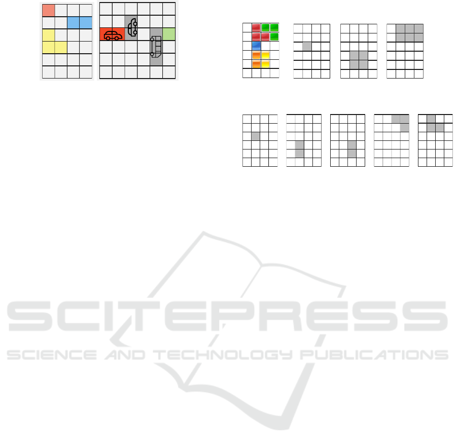
Figure 1: Example of a Tetris problem instance with 1 block

of each type (left) and a Rush Hour problem instance with

one small car and one large car (right).

ture has been proposed in (Urbanovsk

a and Komenda,

2023) where the authors use a tensor representation

motivated by the problems’ semantics to train the se-

mantically layered CSRN (slCSRN). The architec-

tures trained in this work are all based on the architec-

ture described in (Urbanovsk

a and Komenda, 2023).

However, the number of problem domains avail-

able for the semantically layered representation pro-

posed in (Urbanovsk

a and Komenda, 022a) is still

limited. Therefore, in this work, we extend the

number of available domains by the Tetris and

Rush Hour planning domains and propose their one-

layer and multi-layer semantically layered representa-

tions. These domains differ from the existing (maze,

Sokoban) domains since they do not have one explic-

itly deﬁned agent who performs all the actions, but

they contain independent movement of different ob-

jects in the problem. We train the slCSRN archi-

tecture variants for both of these domains and com-

pare their performance with existing classical plan-

ning heuristics. We also analyze the computation of

the architectures and provided several insights into

what are the slCSRNs actually learning. That way

we can make a step towards AI explainability, which

we consider an important feature of machine learning

in the modern days.

2 PROBLEM DOMAINS

We use two problem domains in this work. The ﬁrst

one is Tetris domain, inspired by the famous puzzle

game. This problem domain has been used in the

International Planning Competition. In the planning

version of Tetris, there are three types of blocks (1×1,

2 × 1, and an L block) that are randomly placed on a

grid as shown in Figure 1. The goal is to rotate and

move the blocks, so they all ﬁt into the bottom half of

the grid, leaving the top half of the grid empty.

The second problem domain is the Rush Hour

puzzle, inspired by the already existing board game.

In Rush Hour, there is a 6 × 6 grid map that contains

randomly placed small (1 × 2) and large (1 × 3) cars

that are blocking the route for the red car that you

Tetris

in 2D

0 0 0 0

0 1 0 0

0 0 0 0

1x1 layer 2x1 layer

L layer

0 0 0 0

0 1 1 0

0 0 0 0

0 1 1 1

0 0 0 0

Tetris in semantically layered

representation - one- layer

0 0 0 0

0 1 0 0

0 0 0 0

1x1 layer

2x1 layer

L layer

Tetris in semantically layered

representation - multi- layer

0 0 0 0

0 1 0 0

0 0 0 0

0 0 1 1

0 0 0 1

0 0 0 0

2x1 layer

0 0 0 0

0 0 1 0

0 0 0 0

L layer

0 1 0 0

0 1 1 0

0 0 0 0

Figure 2: Semantically layered representation for a Tetris

problem instance - both one-layer and multi-layer represen-

tation.

have to slide across the whole grid to reach the exit.

The complexity of this puzzle is P-SPACE complete

(Flake and Baum, 2002).

Both of the used problems do not contain a single

agent that performs the actions. We can also think of

these problems as of multi-agent ones.

Next, we introduce the one-layer and multi-layer

semantical representations for both of these problem

domains. All described representations also follow

the rules stated in (Urbanovsk

a and Komenda, 2023)

and before the semantically layered representation

acts as an input to the slCSRN, we pad it with ”walls”

and add one layer for this padding.

2.1 Tetris Representation

The Tetris domain has an explicitly deﬁned grid in its

PDDL representation by stating a number of grid cells

and their connections. The one-layer representation

depends on the number of object types in the problem.

In this case, we have three types of blocks. Therefore,

the one-layer representation has one layer for every

block type. That creates a quite compact input, but it

can also cause problems when distinguishing the in-

dividual blocks of one type, as shown in (Urbanovsk

and Komenda, 022a).

The multi-layer representation has a number of

layers equal to the number of individual blocks. The

representation can get a lot larger compared to the

one-layer one, but each block has its layer and can

be identiﬁed without problems, which gives us more

information about the individual blocks. Both repre-

sentations are shown in Figure 2.

Explainability Insights to Cellular Simultaneous Recurrent Neural Networks for Classical Planning

593

Rush Hour

in 2D

EXIT

Rush Hour in semantically

layered representation - one- layer

0 0 0 0

0 0 1 0

1 1 1 0

0 0 0 0

0 0

small car layer

0 1 1 1

0 0 0 0

0 0

1 0

0 0

large car layer

Rush Hour in semantically

layered representation - multi- layer

0 0 0 0

1 1 0 0

0 0 0 0

0 0

small car layer

0 1 1 1

0 0 0 0

0 0

large car layer

0 0 0 0

0 0 1 0

0 0 0 0

0 0

small car layer

0 0 0 0

0 0

1 0

0 0

large car layer

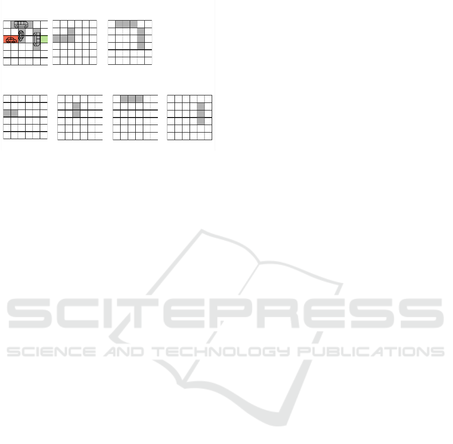
Figure 3: Semantically layered representation for a Rush

Hour problem instance - both one-layer and multi-layer rep-

resentation.

2.2 Rush Hour Representation

The Rush Hour puzzle is played on a 6× 6 grid, how-

ever, the problems can be created on an arbitrarily

sized grid with an arbitrary number of cars. The size

of the grid is deﬁned in the PDDL similarly to the

Tetris grid. The number of object types in this case

is only two. Therefore, in the one-layer representa-

tion, we have two layers, each for one type of car.

In the layer with small cars (1 × 2), we also place the

”red car” which is the most important one in the game

since it is the car that has to exit the map. The next

layer is for the large cars (1 × 3).

The multi-layer representation has one layer for

every car. That has a clear advantage for the ”red car”

that is easier to identify in this representation. Both

representations are shown in Figure 3.

3 TRAINING

We used the exact architecture as proposed in (Ur-

banovsk

a and Komenda, 2023). That allowed us to

train 4 versions of the slCSRN architecture

• slCSRN with one-layer representation

• slCSRN with multi-layer representation

• unfolded slCSRN with one-layer representation

• unfolded slCSRN with multi-layer representation

Differences between the representations are de-

scribed in Section 2. The slCSRN uses weight sharing

among its recurrent networks, the unfolded slCSRN

uses one set of weights for one recurrent iteration.

Another parametrization of the training comes

from the architecture itself, as we can set the number

of recurrent iterations and hidden states of the archi-

tecture. We stuck to the previous works that used the

combinations of parameters

• number of recurrent iterations = [10, 20, 30]

• number of hidden states = [5, 15, 30]

The loss function used for training is the mono-

tonicity inducing loss as proposed in (Urbanovsk

and Komenda, 2021) that focuses rather on the mono-

tonicity of the learned heuristic values rather than on

the absolute values themselves. All the conﬁgurations

were trained for 2000 epochs.

The training data for both domains were generated

randomly. Tetris training data was of size 2 × 2 and

4 × 2 with 1 − 4 blocks. The Rush-Hour training data

was of size 3 × 3, 3 × 4, 4 × 3, and 4×4 with up 2 − 5

small cars and 0 − 2 large cars placed on the map.

As labels, we used the optimal solution lengths

that we acquired using the Breadth-ﬁrst Search algo-

rithm.

For every slCSRN version, we selected the best

conﬁguration for the planning experiments. The se-

lected conﬁgurations for both problem domains are

shown in Table 1.

4 PLANNING EXPERIMENTS

The planning experiments are performed by using

the selected trained slCSRN architectures as heuris-

tic functions in a search algorithm. Similarly to the

previous works, we are using the Greedy Best-ﬁrst

Search that uses solely the heuristic value to guide the

search.

It is not our main goal to outperform any ex-

isting heuristics, we simply want to see the perfor-

mance of the machine learning-based approaches to

see the comparison and get more insight into the

learned heuristic functions. We run the experiments

of the blind heuristic, h

max

(Bonet and Geffner, 2001),

add

(Bonet and Geffner, 2001) and h

(Hoffmann,

2001).

The blind heuristic serves as a baseline that gives

us the equivalent of a random search, as it always re-

turns 0 for any state. The other three heuristic func-

tions are widely used in the ﬁeld of classical planning.

slCSRN and unfolded slCSRN conﬁguration used in

these experiments are shown in Table 1.

The planning experiments were performed on one

dataset for each domain with 50 problem instances.

Each problem instance had a time limit of 10 min-

utes. We used 3 metrics to compare the results. The

most important one is coverage (cvg) which shows the

percentage of solved problems from the given set. It is

commonly used in classical planning. Other than that,

ICAART 2024 - 16th International Conference on Agents and Artiﬁcial Intelligence

594

Table 1: Selected slCSRN and unfolded slCSRN architectures for each semantically layered representation of Tetris and Rush

hour. These will be further used in the planning experiments.

Tetris Rush hour

Architecture Representation Recurrent iterations Hidden states Recurrent iterations Hidden states

slCSRN one-layer 10 5 20 30

slCSRN multi-layer 10 30 10 30

unfolded slCSRN one-layer 20 30 10 5

unfolded slCSRN multi-layer 10 5 10 30

Table 2: Planning experiments for the Tetris domain. All

the best results are in bold lettering. The slCSRN architec-

ture input representation is denoted ol for one-layer and ml

for multi-layer. This representation is followed by architec-

tures’ parameters.

Tetris

avg pl avg ex cvg

blind 4.55 4045.26 0.84

max

5.16 471.63 0.98

add

5.14 18.08 0.98

5.73 36.57 0.98

slCSRN-ol-10-5 4.21 4.38 0.48

slCSRN-ml-10-30 8.10 19.29 0.62

unfolded slCSRN-ol-20-30 4.35 4.74 0.46

unfolded slCSRN-ml-10-5 8.30 11.5 0.6

Table 3: Planning experiments for the Rush Hour domain.

All the best results are in bold lettering. The slCSRN ar-

chitecture input representation is denoted ol for one-layer

and ml for multi-layer. This representation is followed by

architectures’ parameters.

Rush Hour

avg pl avg ex cvg

blind 73.81 5210.19 0.96

max

74.62 2765.02 0.96

add

77.21 3343.23 0.94

76.61 2765.53 0.98

slCSRN-ol-20-30 84.3 3580.9 0.8

slCSRN-ml-10-30 81.49 4952.08 0.78

unfolded slCSRN-ol-10-5 86.68 5035.64 0.94

unfolded slCSRN-ml-10-30 83.95 4104.16 0.76

we also use the average plan length (avg pl) and the

average number of expanded states (avg ex) to gain

more information.

The dataset used in these experiments contains

problem instances that were not present in the training

data, and the grids are larger than the training sam-

ples for both the Tetris and the Rush Hour domain.

The Tetris grids in this set are of sizes 4 × 4 and 6 × 4

with 3 − 6 blocks. The Rush Hours problem instances

are all on 6 ×6 grid and were taken from the database

available at (Fogleman, 2023). We took the 50 puz-

zles with the longest solutions that contained no walls

for the planning dataset.

The complete results can be seen in Table 2 for the

Tetris domain and Table 3 for the Rush Hour domain.

4.1 Tetris Result Discussion

The results of the planning experiment in Table 2

show that the coverage metric is a lot lower than in

the case of classical planning heuristics. This can be

caused by multiple things, including computational

time, therefore we decided to provide a further anal-

ysis of the planning results for the Tetris domain by

comparing each learned heuristic with the classical

planning heuristics separately only using the solved

problem instances. That way, we can compare each

trained slCSRN version fairly and see if there is any

advantage in its performance in terms of the other

metrics.

Table 4: More detailed analysis of the Tetris planning ex-

periments results for each conﬁguration’s solved instances.

Each section of the table relates to the corresponding slC-

SRN conﬁguration and the best results are in bold lettering.

Tetris

avg pl avg ex

max

3.71 25.92

add

3.58 8.21

4.08 13.67

slCSRN-ol-10-5 4.21 4.38

max

4.03 113.45

add

4.0 12.68

4.52 13.58

slCSRN-ml-10-30 8.1 19.29

max

3.61 15.74

add

3.52 6.48

4.0 9.96

unfolded slCSRN-ol-20-30 4.35 4.74

max

4.1 240.47

add

4.03 15.4

4.63 25.0

unfolded slCSRN-ml-10-5 8.3 11.5

Even though the overall coverage does not seem

very impressive for the learned heuristics for the

Tetris domain, we can see that the individual learned

heuristics are performing greatly in the instances they

solved. In Table 4, we can see that three out of the

four trained slCSRN versions dominate in the average

number of expanded states.

That means that the learned heuristics were able

to navigate the search algorithm more reliably than

the classical planning heuristics. Since we are using a

Explainability Insights to Cellular Simultaneous Recurrent Neural Networks for Classical Planning

595

greedy search algorithm, the path length comparison

does not carry a lot of importance since the search

does not have a guarantee on the solutions’ length.

4.2 Rush-Hour Result Discussion

Results for the Rush-Hour domain can be seen in Ta-

ble 3. In this case, the coverage is much closer to

the classical planning heuristics. We can see that the

unfolded slCSRN that uses one-layer representation

was able to achieve 94% coverage, which is on par

with the classical planning heuristics. Even the ar-

chitecture with the least coverage was able to solve

76% of the problems. Both average path length and

average number of expanded states are between the

blind search and the other classical planning heuris-

tics. That implies that the learned heuristics are work-

ing better than no heuristic at all, but their informa-

tiveness does not seem to be up to the classical heuris-

tic standards.

5 EXPLAINABILITY INSIGHTS

The explainability of Artiﬁcial Intelligence is an im-

portant and well-discussed topic. Many methods have

been developed to support explainability on images

(Haar et al., 2023) or for large language models (Zhao

et al., 2023). However, there are not many approaches

that would be usable on a recurrent message passing

architecture such as slCSRN. Therefore, we wanted to

approach the explanation a little more intuitively and

provide some insights into the slCSRN computations

using classical planning. We would also like to men-

tion that this analysis does not fully explain the per-

formance of the individual trained models in the plan-

ning experiments, but rather provides a deeper under-

standing of the heuristic computation by the slCSRN.

To keep the results compact, we decided to per-

form the explainability analysis with the trained net-

works chosen for the planning experiments for both

problem domains.

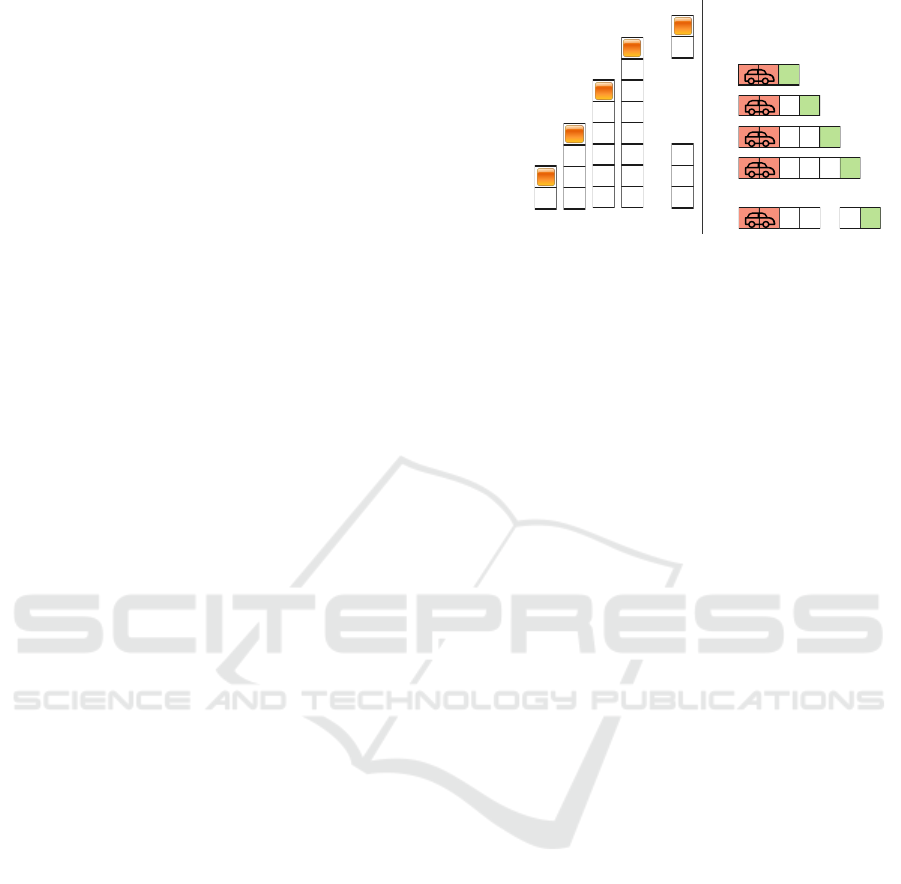
We used the same strategy for both problem do-

mains. We created a very simple toy problem instance

with only one movable object that was solvable sim-

ply by moving it in one direction for a number of

steps.

The toy problem for the Tetris domain is shown in

Figure 4. The problem consisted of only one square

block and a long, narrow path. The smallest instance’s

path length was one, the longest was 30. The ﬁnal

size 30 was taken from the maximum number of re-

current iterations that we used in the training of the

models. For each of these created instances, we gen-

...

Plan

length

1 2

3 4

EXIT

...

Plan

length

Tetris

Rush Hour

Figure 4: Toy data for Tetris (left side) and Rush Hour (right

side) used for the explainability analysis. We can see the

plan length near each problem instance.

erated all possible states starting from the given in-

stance and also saved the number of steps needed to

solve each state.

For the Rush Hour domains, the dataset was cre-

ated accordingly as shown in Figure 4. The smallest

instance only requires one step to reach the goal, the

largest instance requires 30 steps.

The next step is letting the slCSRN architecture

compute a heuristic value for every single generated

state in the dataset. This data can be shown in a plot

for each sample to see the slCSRN behavior for every

problem instance over all of its states.

We can see an example of this plot in Figure 5

where each line consists of heuristic values computed

by the corresponding slCSRN for the Tetris domain.

We can see that the architecture converged to a certain

pattern in that has been satisfactory for the loss func-

tion during the training. This behaviour has been the

same for all the architectures.

The same plots for the Rush Hour domain can be

seen in Figure 7. Each line in the graph represents

one problem instance, and each value along the way

shows the heuristic estimate at the given number of

steps away from the goal. In this case, we do not see

the patterns that were obvious for the Tetris domain,

but we can see that the variance of the generated val-

ues greatly differs across the models.

To learn more about the actual quality of the

heuristic and not just the shape of the learned heuris-

tic function, we can take the heuristic values for each

problem instance and for every state on the way from

the initial state to the goal and compare it to its neigh-

boring values. As we already mentioned, the loss

function we used is focused on monotonicity. There-

fore, we can count how many heuristic values for each

number of steps are correctly placed within the array

of values. In Figure 6, we can see that the mono-

tonicity over the different number of steps to the goal

is not very high overall. We see that the majority of

correctly generated values in terms of monotonicity

appear very close to the goal. For the rest of the path,

ICAART 2024 - 16th International Conference on Agents and Artiﬁcial Intelligence

596

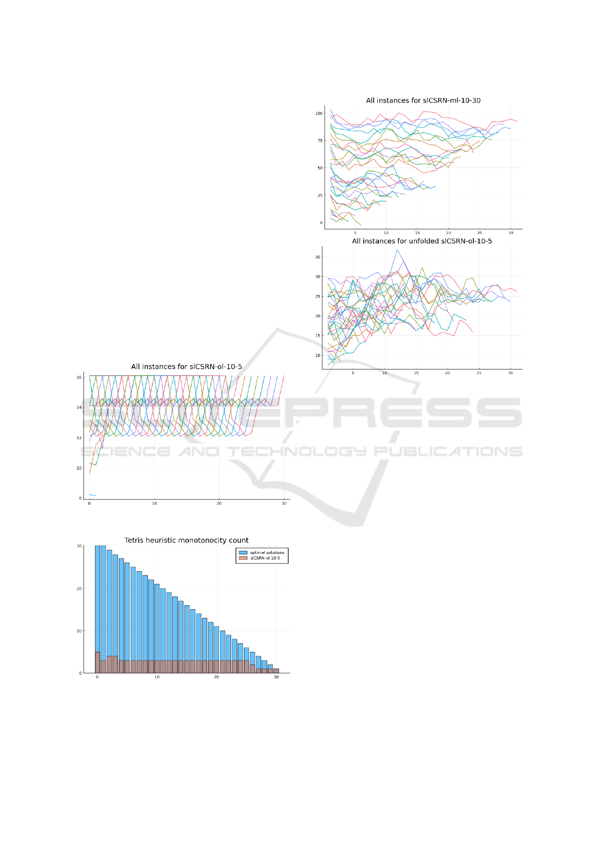
the architecture is rather uncertain about the goal dis-

tance estimate and does not place the heuristic values

in the correct order very often.

In the case of the Rush Hour domain, we can see in

Figure 8 that the number of correctly placed heuristic

values slightly differs for each displayed architecture

version. We can assume that high values mark par-

ticular distances, where the network makes a decision

that is statistically important for the search.

The slCSRN-ml-10-30 was the weakest of these

four architectures in terms of performance in the plan-

ning experiments. We can see the highest number

of correctly generated values around 6–7 steps from

the goal, but before and after the values are very low,

which could cause the performance issues.

The unfolded slCSRN-ol-10-5 has quite a high

number of correctly generated heuristic values up to

11 steps away from the goal. That implies that the

navigation is a lot more reliable around the goal and

once the number of steps needed to solve the prob-

lem goes higher, the network does not provide a very

reliable estimate.

Figure 5: Heuristic values for the Tetris explainability

dataset.

Figure 6: Monotonicity counts for the Tetris heuristic val-

ues. The blue values show numbers for the perfect mono-

tonicity, the orange values are achieved by the correspond-

ing slCSRN.

Figure 7: Heuristic values for the Rush Hour explainability

dataset.

5.1 Explainability Discussion

Overall, we can see that the training had a different

effect on each of the two domains. Let us discuss

the possible outcomes of the proposed explainability

analysis.

The architectures trained on the Tetris domain

learned a repetitive pattern that occurs for instances

of various plan lengths shown in Figure 5. This might

imply that there really is a simple algorithm-like pat-

tern generating heuristic values for this problem do-

main. On the other hand, this pattern can also be

caused by any problem in the training dataset, just as

an insufﬁcient amount of training samples that cause

overﬁtting.

The Rush Hour sample analysis shown in Figure 7

seems to have a better representation of the networks’

computations, and the monotonicity counting analy-

sis indicated that the number of steps estimable by

the models is certainly limited. However, even the

less informed estimates far away from the goal can

be informative for the search algorithms. We can see

that the estimates further from the goal are forming

smoother curves, and therefore the values are less ac-

curate, which is caused by the limited number of iter-

ations of the slCSRN architecture.

Another insight based on the explainability analy-

sis can be read as the ability of the learning process to

Explainability Insights to Cellular Simultaneous Recurrent Neural Networks for Classical Planning

597

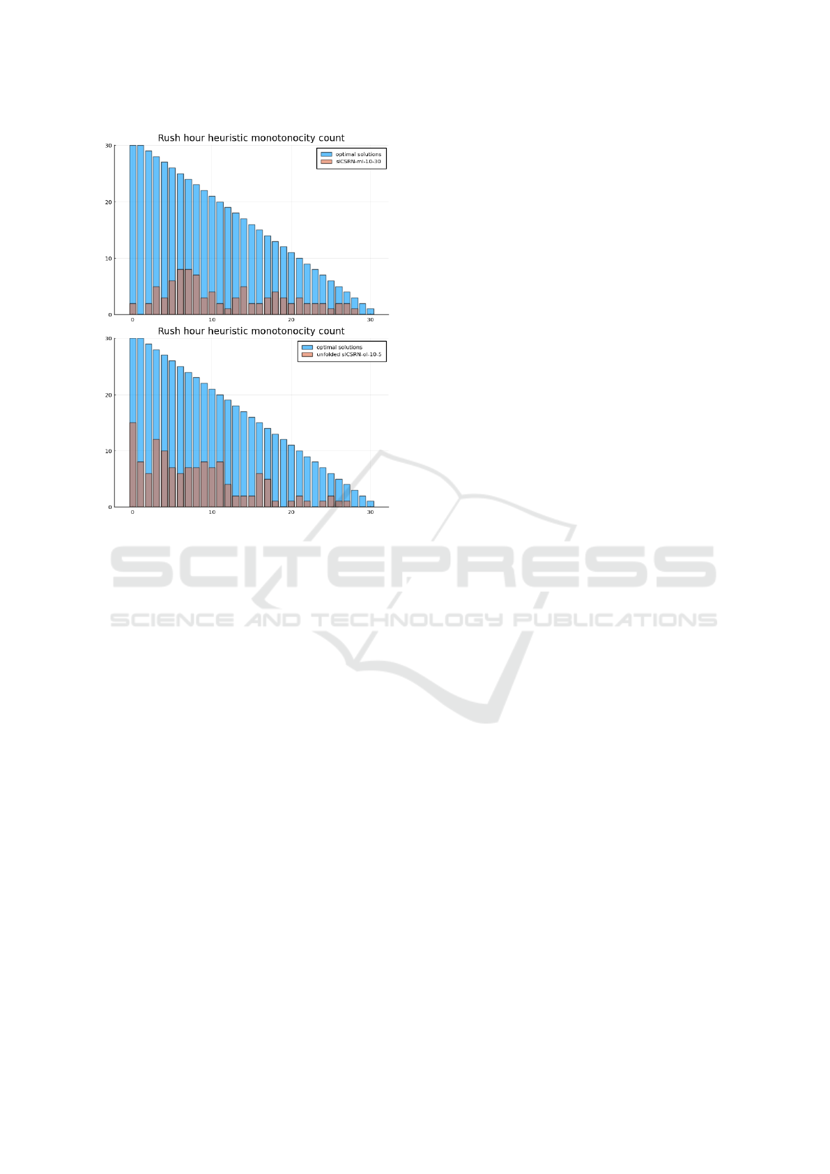
Figure 8: Monotonicity counts for the Rush Hour heuris-

tic values. The blue values show numbers for the perfect

monotonicity, the orange values are achieved by the corre-

sponding slCSRN.

reﬂect the need for a more systematic or randomized

approach to solve different planning problems. On the

one hand, the Tetris problems need a more systematic

approach, as the problem is not overly constrained.

The Tetris pieces are in most cases loose and mov-

able in all directions, only with the exception, of when

they are getting stacked to the goal part of the grid.

On the other hand, the cars in the Rush Hour are al-

ways highly constrained in movement, (a) only in two

directions, (b) by other cars around. The more con-

strained problems are more easily solvable by more

randomized strategies. Intuitively, if we ”randomly

shufﬂe” the Rush Hour puzzle with a bias toward the

goal, we will have a higher chance of solving the

problem than if we randomly shufﬂe the Tetris do-

main, where we will only get most of the pieces into

the empty part of the grid and jiggle them around their

positions (that will happen even with a bias towards

the goal area because some pieces have to wait for

correct positioning of others).

The Table 2 exhibits low coverage results, as for

the machine-learning-based heuristics it is more com-

plicated to learn systematic heuristic evaluation, than

randomization. However, as Table 3 shows, in the

case of Rush Hour the randomization gets on par in

the coverage of the solved problems with the classi-

cal systematic heuristics as h

max

, h

add

, h

. A similar

pattern can be seen in the explainability analysis of

the heuristic values in Figure 7, which exhibits clearly

noisy behavior in Rush Hour, especially for the best

performing network unfolded slCSRN-ol-10-5. In the

case of Tetris, the neural network, however, behaves

systematically, providing a repetitive pattern of the

heuristic values estimation based on the distance from

the goal.

6 CONCLUSION

We have successfully tested the set of available do-

mains for heuristic learning by slCSRN architecture

on two domains — Tetris and Rush Hour. Both of

these domains show properties different from the do-

mains previously used with slCSRN as they contain

multiple movable objects that inﬂuence the available

actions of many different objects in the problem.

We have trained both slCSRN and unfolded slC-

SRN architectures with both one-layer and multi-

layer semantically layered representations for both of

the domains. We also compared the performance of

these trained models in a heuristic search to classical

planning heuristic functions.

On top of that, we analyzed the behavior of the

trained models and created an explainability tech-

nique that allows us to describe the behavior. We cre-

ated an explainability dataset consisting of differently

sized levels of a simple toy problem that allowed us to

analyze how the networks behave regarding the plan

length. With this dataset, we analyzed the shape of the

learned heuristic functions and also the monotonicity

of produced values. These insights gave us a better

idea of what the models learn and how the learning

differs for domains requiring more systematic or ran-

domized heuristic functions.

In the future,

In the future, a potential direction could involve

focusing on domains that are not explicitly deﬁned on

a grid and creating a universal translating algorithm

for any PDDL problem into a semantically layered

representation. Moreover, there is an interest in on-

going exploration of the explainability ﬁeld, examin-

ing diverse methods that might contribute to a deeper

understanding of these approaches.

ACKNOWLEDGEMENTS

The work of Michaela Urbanovsk

a was supported

by the European Union’s Horizon Europe Research

and Innovation program under the grant agreement

ICAART 2024 - 16th International Conference on Agents and Artiﬁcial Intelligence

598

TUPLES No 101070149 and by the Grant Agency

of the Czech Technical University in Prague, grant

No. SGS22/168/OHK3/3T/13. The work of Anton

ın

Komenda was supported by the Czech Science Foun-

dation (grant no. 22-30043S).

REFERENCES

Asai, M. and Fukunaga, A. (2017). Classical planning in

deep latent space: From unlabeled images to PDDL

(and back). In Besold, T. R., d’Avila Garcez, A. S.,

and Noble, I., editors, Proceedings of the Twelfth In-

ternational Workshop on Neural-Symbolic Learning

and Reasoning, NeSy 2017, London, UK, July 17-18,

2017, volume 2003 of CEUR Workshop Proceedings.

Asai, M. and Fukunaga, A. (2018). Classical planning in

deep latent space: Bridging the subsymbolic-symbolic

boundary. In Thirty-Second AAAI Conference on Ar-

tiﬁcial Intelligence.

Asai, M. and Muise, C. (2020). Learning neural-symbolic

descriptive planning models via cube-space priors:

The voyage home (to STRIPS). In Bessiere, C., editor,

Proceedings of the Twenty-Ninth International Joint

Conference on Artiﬁcial Intelligence, IJCAI 2020,

pages 2676–2682. ijcai.org.

Bonet, B. and Geffner, H. (2001). Planning as heuristic

search. Artiﬁcial Intelligence, 129(1-2):5–33.

Flake, G. and Baum, E. (2002). Rush hour is pspace-

complete, or “why you should generously tip park-

ing lot attendants”. Theoretical Computer Science,

270:895–911.

Fogleman, M. (2023). Rush hour instance database.

Ghallab, M., Knoblock, C., Wilkins, D., Barrett, A., Chris-

tianson, D., Friedman, M., Kwok, C., Golden, K.,

Penberthy, S., Smith, D., Sun, Y., and Weld, D.

(1998). Pddl - the planning domain deﬁnition lan-

guage.

Groshev, E., Tamar, A., Goldstein, M., Srivastava, S., and

Abbeel, P. (2018). Learning generalized reactive poli-

cies using deep neural networks. In 2018 AAAI Spring

Symposium Series.

Haar, L. V., Elvira, T., and Ochoa, O. (2023). An analy-

sis of explainability methods for convolutional neural

networks. Engineering Applications of Artiﬁcial In-

telligence, 117:105606.

Hoffmann, J. (2001). Ff: The fast-forward planning system.

AI magazine, 22(3):57–57.

Ilin, R., Kozma, R., and Werbos, P. J. (2008). Beyond feed-

forward models trained by backpropagation: A prac-

tical training tool for a more efﬁcient universal ap-

proximator. IEEE Transactions on Neural Networks,

19(6):929–937.

Shen, W., Trevizan, F. W., and Thi

ebaux, S. (2020). Learn-

ing domain-independent planning heuristics with hy-

pergraph networks. In Beck, J. C., Buffet, O., Hoff-

mann, J., Karpas, E., and Sohrabi, S., editors, Pro-

ceedings of the Thirtieth International Conference on

Automated Planning and Scheduling, Nancy, France,

October 26-30, 2020, pages 574–584. AAAI Press.

ahlberg, S., Bonet, B., and Geffner, H. (2021). Learning

general optimal policies with graph neural networks:

Expressive power, transparency, and limits. CoRR,

abs/2109.10129.

ahlberg, S., Bonet, B., and Geffner, H. (2022). Learning

generalized policies without supervision using gnns.

In Kern-Isberner, G., Lakemeyer, G., and Meyer, T.,

editors, Proceedings of the 19th International Confer-

ence on Principles of Knowledge Representation and

Reasoning, KR 2022, Haifa, Israel, July 31 - August

5, 2022.

ahlberg, S., Bonet, B., and Geffner, H. (2023). Learn-

ing general policies with policy gradient methods. In

Marquis, P., Son, T. C., and Kern-Isberner, G., editors,

Proceedings of the 20th International Conference on

Principles of Knowledge Representation and Reason-

ing, KR 2023, Rhodes, Greece, September 2-8, 2023,

pages 647–657.

Toyer, S., Thi

ebaux, S., Trevizan, F. W., and Xie, L. (2020).

Asnets: Deep learning for generalised planning. J.

Artif. Intell. Res., 68:1–68.

Urbanovsk

a, M. and Komenda, A. (2021). Neural net-

works for model-free and scale-free automated plan-

ning. Knowledge and Information Systems, pages 1–

36.

Urbanovsk

a, M. and Komenda, A. (2022a). Grid represen-

tation in neural networks for automated planning. In

Rocha, A. P., Steels, L., and van den Herik, H. J., edi-

tors, Proceedings of the 14th International Conference

on Agents and Artiﬁcial Intelligence, ICAART 2022,

Volume 3, Online Streaming, February 3-5, 2022,

pages 871–880. SCITEPRESS.

Urbanovska, M. and Komenda, A. (2023). Analysis of

learning heuristic estimates for grid planning with cel-

lular simultaneous recurrent networks. SN Computer

Science, 4.

Urbanovsk

a, M. and Komenda, A. (2023). Semantically

layered representation for planning problems and its

usage for heuristic computation using cellular simul-

taneous recurrent neural networks. In Rocha, A. P.,

Steels, L., and van den Herik, H. J., editors, Proceed-

ings of the 15th International Conference on Agents

and Artiﬁcial Intelligence, ICAART 2023, Volume 3,

Lisbon, Portugal, February 22-24, 2023, pages 493–

500. SCITEPRESS.

Zhao, H., Chen, H., Yang, F., Liu, N., Deng, H., Cai, H.,

Wang, S., Yin, D., and Du, M. (2023). Explain-

ability for large language models: A survey. CoRR,

abs/2309.01029.

Explainability Insights to Cellular Simultaneous Recurrent Neural Networks for Classical Planning

599