
A New Algorithm for Innervation Zone Estimation Using Surface
Electromyography: A Simulation Study Based on a Simulator for
Continuous sEMGs
Malte Mechtenberg
1,2 a
, Nils Grimmelsmann
1,2 b
and Axel Schneider
1,2 c
1
Biomechatronics and Embedded Systems Group, University of Applied Sciences and Arts, Bielefeld, NRW, Germany
2
Institute of System Dynamics and Mechatronics, University of Applied Sciences and Arts, Bielefeld, NRW, Germany
Keywords:
Innervation Zone, Muscle, Innervation Point, EMG, EMG Simulation, Electromyography, Motor Unit, Firing
Pattern, EMG Array.
Abstract:
In this work, a novel algorithm for the estimation of the innervation zone location within a muscle head is
presented. The algorithm is able to identify innervation zone clusters within continuous surface electromyog-
raphy (sEMG) recordings based on linear electrode arrays. The presented algorithm is tested in a simulation
environment, which is capable of simulating EMG signals based on a common drive signal (activation). The
simulator was used to generate sEMGs of six virtual muscle based on six different configurations for the re-
spective muscle fibre distributions. The virtual muscles were each activated with a trapezoidal signal (common
drive). The new algorithm was able to identify the location of the innervation zone centers with a mean ab-
solute error of 3.8% of the inter electrode distance. In the best case, the absolute error was below 1 % of the
inter electrode distance.
1 INTRODUCTION
This work introduces a new algorithm for the esti-
mation of innervation zones in an electromyography
recording. It is based on a previously published al-
gorithm (Mechtenberg and Schneider, 2023) that was
only able to find one innervation zone location per
EMG recording, thus requiring manual labor when
multiple innervations zone locations have to be identi-
fied in a recoding. The novel extension presented here
allows an automatic detection of multiple innervation
zone locations within one recording. Thus being com-
parable to other methods presented in the litrature,
that are for example (Mesin et al., 2009; Beck et al.,
2012; Marateb et al., 2016; Huang et al., 2023). The
method presented here has a small parameter set and
an implementation that is available as open source
software (Apache 2.0 license) (Mechtenberg, 2023b).
A Brief Introduction to Innervation Zones. Mus-
cle fibres of skeletal muscles are controlled by so-
called motor neurons which are situated in the pe-
a
https://orcid.org/0000-0002-8958-0931
b
https://orcid.org/0000-0002-4864-4978
c
https://orcid.org/0000-0002-6632-3473
ripheral nervous system within the spine. A motor
neuron connects to several muscle fibres. The combi-
nation of muscle fibres and a motor neuron is called
a motor unit. An axon of a motor neuron connects to
the respective muscle fibre at the so-called innervation
points (IPs) via the motor end plates. The innervation
points of a motor unit are distributed over the muscle
body. This distribution of IPs is called the innervation
zone (IZ) of the motor unit. The IZ locations vary
considerably between subjects (Guzm
´
an et al., 2011).
Moreover, during contraction, the length and position
changes of the muscle also change the relative posi-
tion of the IZs (Piitulainen et al., 2009; Martin and
MacIsaac, 2006).
In summary, the IZ location is specific for a sub-
ject and experiment condition. This means it is hard
to follow heuristics, based for example on anatomi-
cal measures to localize the IZ. An attempt was made
with an atlas of innervation zones (Barbero et al.,
2012). This atlas is considered as a general reference
for the distribution of IZs between multiple subjects.
It is, however, lacking when precise knowledge of the
inervation zone is needed, as for example in the fol-
lowing scenarios.
Mechtenberg, M., Grimmelsmann, N. and Schneider, A.
A New Algorithm for Innervation Zone Estimation Using Surface Electromyography: A Simulation Study Based on a Simulator for Continuous sEMGs.
DOI: 10.5220/0012375100003657
Paper published under CC license (CC BY-NC-ND 4.0)
In Proceedings of the 17th International Joint Conference on Biomedical Engineering Systems and Technologies (BIOSTEC 2024) - Volume 1, pages 629-636
ISBN: 978-989-758-688-0; ISSN: 2184-4305
Proceedings Copyright © 2024 by SCITEPRESS – Science and Technology Publications, Lda.
629

Σ
intra
muscular
EMG
sensor
activation
{
{
∆t
∆t
CD(t)
t
m
I (t)
t
s
t
n
e
v
e
n
o
i
t
a
v
i
t
c
a
Figure 1: Representation of a motor unit pool consisting of several motor units (green and blue) that are triggered by a
common drive (CD) signal (trapezoidal, top left). The times between individual firing events (∆t) are drawn from normal
distributions with the corresponding mean frequency and standard deviations as described in eqs. (1) and (2). The simulator
determines the measurable potentials on the skin surface (EMG sensor, top right) from the temporal course of all firing events
(respectively the corresponding spread of the motor unit action potentials on the muscle fibres).
Possible Applications of Precision IZ Location
Estimation. The precise localization of innervation
zones is of interest for example in:
• medical treatments, when drugs have to be deliv-
ered close to the motor end plates (Zhang et al.,
2016).
• exoskeletal control the observed IZ movement
could be used as a measure for the amount of
muscle shortening (Mechtenberg and Schneider,
2023).
• case of sEMG acquisitions where a consistent sig-
nal quality is required over a wide range of move-
ments and subjects. As the sEMG signal char-
acteristics are different when the recording elec-
trodes are placed close to innervation zones com-
pared to locations above the muscle fiber with no
IZ or muscle fiber end close by.
In general, an accessible and reliable algorithm
to identify the IZ in situ could help to improve
experimental setups involving sEMG recordings.
Over the years, different methods to estimate the
innervation zone location based on sEMGs emerged.
An experienced experimenter is able to detect the
IZs by visual sEMG inspection. There were multi-
ple attempts to automate this process with signal pro-
cessing algorithms (Mesin et al., 2009; Beck et al.,
2012; Marateb et al., 2016). However, these algo-
rithms require the selection of appropriate parame-
ter sets. Tuning them appropriately can be challeng-
ing. Mechtenberg and Schneider proposed a new al-
gorithm for the innervation zone detection which uses
only two parameters. In a simulation study, an opti-
mization of these two parameters was performed suc-
cessfully under varying noise conditions (Mechten-
berg and Schneider, 2023). In that study, the algo-
rithm operated only on a single motor unit poten-
tial, i.e. the EMG signal generated by the sum of
all action potentials that travel along the muscle fi-
bres of their respective motor unit. An sEMG record-
ing usually consists of several motor unit potentials
generated from different motor units. In order to
use the proposed algorithm to estimate the innerva-
tion centre in more realistic scenarios (with multi-
ple motor units and activation events), the algorithm
needs to be extended. To test this extension, Mechten-
berg and Schneider’s simulator (Mechtenberg, 2023a)
must also be modified to simulate the activation of
many motor units, resulting in a continuous sEMG.
Both, the extension of the algorithm and of the simu-
lation framework are subject of this work.
The simulator extension is described first in sec-
tion 2.1. The experimental setup is then described
in section 2.2 before the extension of the innervation
zone estimation algorithm is described in section 2.3.
The presented algorithm achieved a mean absolute
error of 0.19mm (SD(AE) = 0.19 mm), that is 3.8%
of the inter electrode distance.
BIOSIGNALS 2024 - 17th International Conference on Bio-inspired Systems and Signal Processing
630

2 METHODS
2.1 Extension of the EMG Simulator
Using the Motor Unit Pool Model
As a basis for the EMG simulation, the approach de-
scribed in (Mechtenberg and Schneider, 2023) was
used. That simulator was only capable of simulating
single motor unit potentials. This means, that several
motor units were only triggered once in the simula-
tion. It was therefore expanded to include the capabil-
ity of generating a continuous EMG signal based on
a continuous muscle activation signal (the common
drive). The concept is depicted in fig. 1. It is sim-
ilar to the approach that was described by (Petersen
and Rostalski, 2019). Here, it was assumed that mo-
tor units are organized in a pool. Such a motor unit
pool is assumed to receive a common activation sig-
nal the common drive (CD). The common drive signal
is always between zero and one, where zero corre-
sponds to no activation and one is the full activation
of a motor unit pool. Each motor unit within a pool is
assumed to start firing from a distinct common drive
level CDS
i
MU
that is unique for each motor unit i
MU
.
The value of CDS
i
MU
follows the size principle as de-
scribed later in this section (see also eq. (3)).
When the i
th
motor unit is active, it generates ac-
tion potentials with a mean firing frequency
¯
f
i
MU
(CD)
that is dependent on the common drive level. The re-
lationship of the mean firing frequency to the com-
mon drive is modeled utilizing eq. (1) as described by
(Petersen and Rostalski, 2019):
¯
f
i
MU
(CD) =
−[c
2
−CD]
·c
1
·CDS
i
MU
+c
3
·CD +c
4
−[c
5
−c
6
·CD]
·e
−
CD−CDS
i
MU
c
7
CDS
i
MU
≤ CD
CD ≤ 1
undefined otherwise
(1)
The actual firing events are generated according to al-
gorithm 1. Once the common drive CD reaches the
starting common drive level CDS
i
MU
of a motor unit,
the time difference of the next firing instance to the
current instance of this motor unit is drawn from a
normal distribution. The mean of that distribution is
defined by
¯
f
i
MU
(CD) (see eq. (1)). The standard devi-
ation of the normal distribution according to (Petersen
and Rostalski, 2019) is
σ
f ,i
MU
(CD) =
10 + 20 ·exp
−
CD−CDS
i
MU
2.5
100 ·
¯
f
i
MU
(CD)
. (2)
Result: motor unit activation pattern
t := time span.start;
while t ≤ time span.end do
CD := CD(t);
if CD ≥ CDS
i
MU
then
∆t := N
1
¯
f
i
MU
(CD)
,σ
f ,i
MU
(CD)
;
add activation event at t + ∆t
else
∆t := 10
−5
;
end
t+ = ∆t ;
end
Algorithm 1: Activation pattern generation of the
i
th
motor unit.
Employment of the Motor Unit Size Principle.
All motor unit parameters, which are not related to
the muscle geometry are assumed to be depended on
the motor unit size. Here, the motor units are ordered
by size, i.e. the smallest motor unit has an index of
i
MU
= 0 and the largest of i
MU
= N
MU
. N
MU
is the
amount of all motor units in the simulated muscle.
This assumption is commonly known as motor unit
size principle. The motor unit parameters that depend
on the motor unit size are the mean conduction veloc-
ity, number of muscle fibres within a motor unit and
the common drive threshold CDS
i
MU
. The relation of
the first two motor unit parameters are described in
(Mechtenberg and Schneider, 2023). The latter is pa-
rameterized by the description of (Petersen and Ros-
talski, 2019), which is an adoption of the motor unit
pool model described by (Fuglevand et al., 1993).
CDS
i
MU
= exp
log(100 ·CDMax
i
MU
)
N
MU
·i
MU
(3)
Where CDMax
i
MU
= 1 was chosen as the the maximal
common drive for a given motor unit.
After the generation of the motor unit firing events
the motor unit potentials are simulated once per mo-
tor unit. Afterwards a motor unit potential train is
generated by shifting the motor unit potentials to the
generated firing events. This shift is done in the dis-
crete time domain. Therefore, the motor unit poten-
tials can not be shifted to the exact time point of each
firing event. Instead, the potentials are shifted to the
discrete point in time that is closest to the respective
firing event. The time resolution is set to the time step
size T = 0.05 ms used during the motor unit potential
simulation.
In a last step, all instances of motor unit potentials
are summed up at each electrode location and down-
sampled to f = 2 kHz.
A New Algorithm for Innervation Zone Estimation Using Surface Electromyography: A Simulation Study Based on a Simulator for
Continuous sEMGs
631
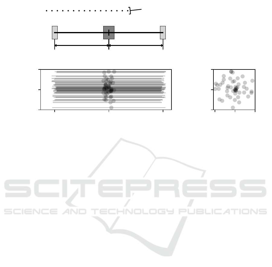
x-axis positions
of the electrode array
W
I
W
T L
W
T R
L
L
L
R
(A)
L
L
P
IZ,x
L
R
x-axis
−R
P
IZ,z
R
z-axis
(B)
−R
P
IZ,y
R
y-axis
−R
P
IZ,z
R
z-axis
(C)
Figure 2: (A) Schematic depiction of the muscle shape defining parameters in the x-axis direction. W
T L
and W
T R
are the width
of the tendon placement regions on the left and right side of the muscle. L
L
and L
R
are the distances between the center of
the innervation zone and the centers of the two tendon regions. The parameter W
I
defines the width of the innervation zone
of the muscle. The location of the motor end plate (innervation point IP) as well as the left and right myotendinous junctions
in the x-axis are drawn from a uniform distribution in these regions. The relative position in the x-axis of the electrodes is
also shown as black dots in the top part. (B, C) depict 50 muscle fibres generated from the setup in (A), where the z- and y-
coordinates of the innervation points are drawn from a uniform circular shaped distribution with the radius R around the center
of the innervation zone. The innervation points are marked with a black dot. The muscle fibres are drawn with a transparency.
2.2 Setup of the EMG Simulation
The simulator in this study can in principle gener-
ate virtual muscle fibres of motor units with differ-
ent lengths (L
L
,L
R
), sizes of the innervation zones
(W
I
) and sizes of tendon regions (W
T L
,W
T R
, loca-
tion of the junction from muscle fibre to tendon) as
shown in fig. 2 (A). These five parameters are called
shape defining parameters. The muscle fibres can be
distributed across a spatial volume with the help of
their position parameters (R, P
IZ,y
,P
IZ,z
, see fig. 2 (B,
C)). For details of the shape defining and position pa-
rameters of the muscle fibres see (Mechtenberg and
Schneider, 2023).
In this study, two scenarios were simulated. Sce-
nario I is displayed in fig. 3 (A) and scenario II in
fig. 3 (B). The shape defining parameters and the mo-
tor unit pool recruitment related parameters are set to
the same values for both scenarios. All constant pa-
rameters are listed in table 1 in the appendix.
In Scenario I, the muscle shape related parameters
W
I
,W
T L
,W
T R
,L
L
,L
R
are kept constant. But the loca-
tion of the whole muscle was shifted along the x-axis
relative to the electrode array (see fig. 3 (A)).
P
IZ,x
∈ {5.75 cm, 4 cm, 1.75 cm} (4)
This way, different innervation zone locations can be
tested with a varying influence of the end effect, that
occurs at the myotendinous junction.
In Scenario II, the muscle shape related parame-
ters L
L
,L
R
and the innervation zone center along the
x-axis were varied. The remaining parameters were
kept constant. L
L
and L
R
were chosen such that the
myotendinous junctions remain at the same position
left and right of the electrode array, as displayed in
fig. 3 (B), while the innervation zone locations were
set to eq. (4).
The virtual electrode array was always placed at
the same position for all scenarios. The electrode
array consists of 16 monopolar electrodes with a
5mm spacing. All electrodes had the same y- and z-
coordinates (table 1). The first electrode in the array
is placed at x = 0 cm.
The result of the simulation is a monopolar record-
ing from a continuous simulated EMG for each mus-
cle based on a trapezoid common drive signal. The
common drive signal that was used is shown in fig. 4.
For the later use of the EMG signal in the al-
gorithm for innervation zone center estimation, the
monopolar recording was converted into a double dif-
BIOSIGNALS 2024 - 17th International Conference on Bio-inspired Systems and Signal Processing
632
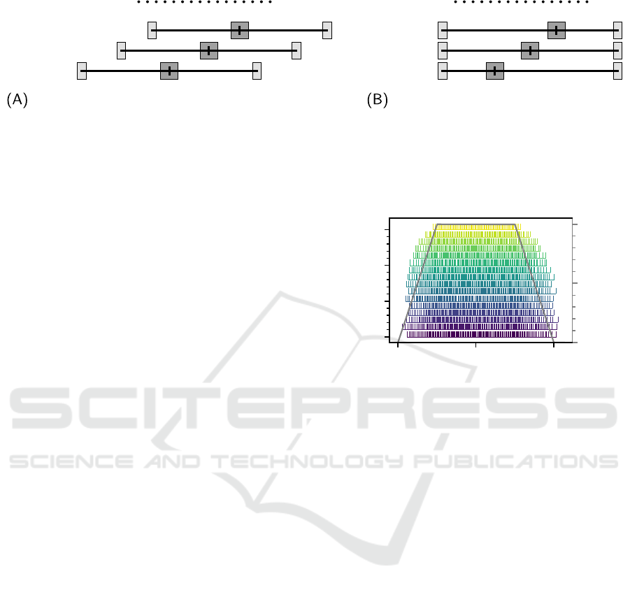
scenario 1 scenario 2
conf. 4
conf. 5
conf. 6
conf. 1
conf. 2
conf. 3
Figure 3: Depiction of the innervation zone and myotendinous junction centers of each simulated virtual muscle relative to
the x-axis position of the electrode array. Two types of innervation zone position shifts were simulated. In (A) the innervation
zone location relative to the virtual muscle stays the same, but the virtual muscle as a whole is shifted along the x-axis relative
to the electrode array. In (B) the myotendinous junction centers remain at the same position on the x-axis, but the innervation
zone centers are shifted relative to the electrode array. In total, six muscle configurations were simulated, all with the same
muscle belly radius R and with the same y-, and z-axis coordinates for the innervation zone center.
ferential recording as described in (Mechtenberg and
Schneider, 2023), resulting in 14 double differential
(DD) EMG signals.
2.3 Innervation Zone Center Estimation
As a basis for the innervation zone center estima-
tion, the algorithm introduced in (Mechtenberg and
Schneider, 2023) was used. That algorithm operates
on a time window of the EMG signal and is able to
find one estimation of the innervation zone center per
time window. The algorithm basically consists of two
steps.
Step 1. Per double differential electrode potential
(one of the above-mentioned 14 DD-signals), one mo-
tor unit potential (MUP) is identified using a wavelet
correlation. This step is parameterized with the
wavelet width λ. As wavelet, the third Hermite-
Rodriguez series expansion was selected, as this was
proposed by (Farina et al., 2000) for the identifica-
tion of double differential MUPs. After identifica-
tion of the motor unit potentials in each of the DD-
signals, the algorithm uses pairs of any combination
of two of those potentials to set up a linear extrapola-
tion (line) that represents the location of the MUPs at
earlier points in time. Since the MUPs travel in both
directions away from the innervation zone, the inter-
section of those extrapolated lines of MUPs that travel
in one direction and those of MUPs that travel in the
other direction represent the innervation zone.
Step 2. The intersection points are clustered using
the density based DBSCAN algorithm (Pedregosa
et al., 2011). The cluster that contains the largest
number of intersections is used to calculate the
innervation zone center location estimate, i.e. the
center of that cluster. This step is parameterized with
0 2 4
time in s
0
250
500
750
motor unit ID
0.0
0.5
1.0
common drive
Figure 4: The activation patterns for every 50th motor unit
within a virtual muscle are shown, with the corresponding
common drive signal that was used to generate the activa-
tion patterns (trapezoidal shape). The color of the firing
events encodes the motor unit size, which also becomes big-
ger with increasing motor unit ID i
MU
.
the density parameter ε of the DBSCAN algorithm.
The result of these two steps is a position rela-
tive to the x-axis of the electrode array and a point in
time. In the previous study (Mechtenberg and Schnei-
der, 2023), a parameter variation was performed in or-
der to find a suitable parameter set, which is tolerant
to noise but still accurate. Based on that work, the pa-
rameters λ = −0.00391667 and ε = 1.10083333 were
selected. For details on the internal paramters please
refer to the publication (Mechtenberg and Schneider,
2023) or the open source implementation of the algo-
rithm (Mechtenberg, 2023b).
Extension to Estimate Innervation Zone Centers
in Continuous EMG Recordings. In this study, the
algorithm described above was extended to operate on
a continuous EMG signal. This extension contains
two aspects.
First, the continuous EMG had to be segmented
into multiple time windows. For that, a 40 ms Hann
window was used. The Hann window reduces the
A New Algorithm for Innervation Zone Estimation Using Surface Electromyography: A Simulation Study Based on a Simulator for
Continuous sEMGs
633
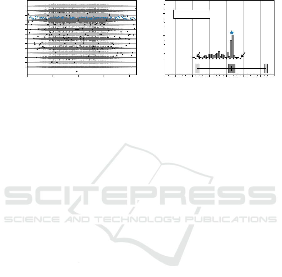
0 1 2 3 4
time in s
DD 0
DD 1
DD 2
DD 3
DD 4
DD 5
DD 6
DD 7
DD 8
DD 9
DD10
DD11
DD12
DD13
(A)
-25 0 25 50 75 100
x coordinate in mm
0
50
100
Count
DD 0 DD 13
AE= 0.02mm
(B)
Figure 5: In (A) all 14 simulated double differential EMG signals for one of the six virtual muscles is displayed. Blue
dots mark the innervation zone location estimates of an innervation zone center cluster. The black dots are innervation zone
estimates, which are not part of a cluster. In (B) the distribution of innervation zone estimates is shown. The blue asterisk
marks the position of the innervation zone cluster center. In the lower part of the plot, the actual innervation zone region and
the myotendinous junction regions are displayed in the same style as in fig. 3. The absolute error from the cluster center (blue
asterisk) and the actual innervation zone center is shown at the top. The absolute error in this case is below 1 % of the inter
electrode distance.
chance that motor unit potentials, which are only
partly within the window, are tracked during Step 1 of
the innervation zone center estimation. The window
was shifted over the EMG signals in 20 ms steps, re-
sulting in 20 ms overlaps. The window width as well
as the window overlap was chosen after inspection of
the motor unit potentials.
For each window, an innervation zone center was
estimated as described above. Second, under the as-
sumption of an isometric contraction, these estimated
positions are clustered in the position domain (axis of
the electrode array) using DBSCAN (Pedregosa et al.,
2011). This leads to an estimate of possible multiple
innervation zone locations per simulation experiment.
The innervation zone center estimation was parame-
terized with eps = 0.1 and min samples = 10.
Per simulation setup presented in fig. 3 the innerva-
tion zone clusters were identified and compared to the
ground truth, i.e. the center of all innervation point lo-
cations.
3 RESULTS
As described, two scenarios with three parameter sets
each were simulated, resulting in six simulated EMGs
(virtual muscles). The input for each simulation was
a common drive (CD) signal in a trapezoidal shape as
displayed in fig. 4 and as depicted as inset in fig. 1.
For all six simulated EMG signals, the extended ver-
sion of the innervation zone estimation algorithm was
applied as described in section 2.3. For one arbitrar-
ily selected of the six virtual muscles a detailed view
on the estimated innervation zones is shown in fig. 5.
In fig. 5 (A) the whole simulated EMG signal is dis-
played with the estimated innervation zone centers for
all time windows. The innervation zone estimates that
are part of the accepted cluster are displayed as blue
dots. The rejected innervation zone estimates are dis-
played in black. In fig. 5 (B) the distribution of in-
nervation zone estimates (compared with (A)) over
the double differential electrode positions is shown,
as well as the center of the accepted cluster (blue as-
terisk). There is a noticeable accumulation of inner-
vation zone centers in the middle of the array. The ac-
cepted innervation zone center is near the maximum
in the histogram and close to the actual innervation
zone center of the simulated muscle (AE= 0.02 mm).
For all simulated virtual muscles, the innervation
zone distribution over the electrodes and the accepted
cluster center are shown in fig. 6. In general, all the
accepted clusters of innervation zone estimates are
close to the actual innervation zone locations. For all
clusters, the difference between their mean estimate
and the actual innervation zone center is below 1 mm.
In case of those virtual muscles with their innervation
zone center close to the middle of the array (2. col-
umn in fig. 6) the error becomes minimal (0.05mm
and 0.08 mm) for both scenarios. The worst value for
the estimation accuracy is 0.56mm.
In case of the simulations where the innervation
zone is close to the end of the array, there seem to be
clusters of false estimates in the middle of the elec-
trode array.
In general, the mean absolute error is MAE =
0.19mm (SD(AE) = 0.19mm).
BIOSIGNALS 2024 - 17th International Conference on Bio-inspired Systems and Signal Processing
634
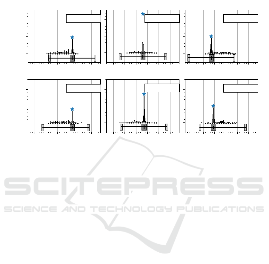
0
50
100
Count
AE= 0.02mm
conf. 1
AE= 0.05mm
conf. 2
AE= 0.28mm
conf. 3
-25 0 25 50 75 100
x coordinate in mm
0
50
100
Count
AE= 0.16mm
conf. 4
-25 0 25 50 75 100
x coordinate in mm
AE= 0.08mm
conf. 5
-25 0 25 50 75 100
x coordinate in mm
AE= 0.56mm
conf. 6
Figure 6: Depiction of the innervation zone location estimate distributions for all six simulated virtual muscles are shown in
the same style as in fig. 5 (B). The blue asterisk marks the center of the accepted innervation zone cluster. All absolute errors
between the cluster centers and the actual innervation zone centers are below 1 mm.
4 DISCUSSION AND
CONCLUSION
This study shows that the newly proposed algorithm
for the innervation zone center estimation can be used
for continuous EMG signals by segmenting the EMG
in overlapping windows. Even with this straight for-
ward approach of segmenting the EMG data, a con-
siderably good result was achieved, since the absolute
prediction error was below 0.57 mm for all tested con-
figurations (MAE = 0.19 mm, SD(AE) = 0.19 mm).
The mean absolute error is 3.8% of the inter electrode
distance 5 mm. This is a result that is close to an-
other recently published innervation zone estimation
algorithm (Huang et al., 2023). Huang et al. report
for their principal component based algorithm a mean
difference of 3 % (up to 8 % depending on the exper-
iment conditions) of the inter electrode distance, that
is 8mm in their setup. For en extensive comparison,
the two algorithmes would have to be evaluated with
the same dataset.
A further result of the investigation was that the
prediction error of the algorithm varies with the elec-
trode array location relative to the innervation zone.
When the electrode array was placed above the inner-
vation zone, a prediction error of AE ≤ 0.05 mm was
achieved. Next steps will include the investigation of
the dependency between the prediction error and dif-
ferent electrode configurations as well as the deriva-
tion of a model which is also able to follow the move-
ment of the innervation zone under different contrac-
tion scenarios of a muscle (e.g. isometric, isotonic
and auxotonic conditions).
ACKNOWLEDGEMENTS
This work has been supported by the research train-
ing group “Dataninja” (Trustworthy AI for Seamless
Problem Solving: Next Generation Intelligence Joins
Robust Data Analysis) and by the “TransCareTech”
project (Transformation in Care & Technology), both
funded by the German federal state of North Rhine-
Westfalia. It was also supported by a Career@Bi
grant of the University of Applied Sciences and Arts,
Bielefeld, Germany.
REFERENCES
Barbero, M., Merletti, R., and Rainoldi, A. (2012). Atlas
of muscle innervation zones: understanding surface
electromyography and its applications. Springer Sci-
ence & Business Media.
A New Algorithm for Innervation Zone Estimation Using Surface Electromyography: A Simulation Study Based on a Simulator for
Continuous sEMGs
635

Beck, T. W., DeFreitas, J. M., and Stock, M. S. (2012). Ac-
curacy of three different techniques for automatically
estimating innervation zone location. Computer meth-
ods and programs in biomedicine, 105(1):13–21.
Farina, D., Fortunato, E., and Merletti, R. (2000). Non-
invasive estimation of motor unit conduction velocity
distribution using linear electrode arrays. IEEE Trans-
actions on Biomedical Engineering, 47(3):380–388.
Fuglevand, A. J., Winter, D. A., and Patla, A. E. (1993).
Models of recruitment and rate coding organization
in motor-unit pools. Journal of neurophysiology,
70(6):2470–2488.
Guzm
´
an, R. A., Silvestre, R. A., Arriagada, D. A.,
GUZM
´
AN, R., SILVESTRE, R., and ARRIAGADA,
D. (2011). Biceps brachii muscle innervation zone lo-
cation in healthy subjects using high-density surface
electromyography. int J Morphol, 29(2):347–52.
Huang, C., Chen, M., Zhang, Y., Li, S., Klein, C. S., and
Zhou, P. (2023). A novel muscle innervation zone esti-
mation method using monopolar high density surface
electromyography. IEEE Transactions on Neural Sys-
tems and Rehabilitation Engineering, 31:22–30.
Marateb, H. R., Farahi, M., Rojas, M., Ma
˜
nanas, M. A.,
and Farina, D. (2016). Detection of multiple innerva-
tion zones from multi-channel surface emg recordings
with low signal-to-noise ratio using graph-cut seg-
mentation. PLoS One, 11(12):e0167954.
Martin, S. and MacIsaac, D. (2006). Innervation zone
shift with changes in joint angle in the brachial bi-
ceps. Journal of Electromyography and Kinesiology,
16(2):144–148.
Mechtenberg, M. (2023a). UAS-Embedded-Systems-
Biomechatronics/EMG-concentrated-current-
sources: v0.2.2.
Mechtenberg, M. (2023b). UAS-Embedded-Systems-
Biomechatronics/sEMG-innervation-zone-
estimation.
Mechtenberg, M. and Schneider, A. (2023). A method for
the estimation of a motor unit innervation zone center
position evaluated with a computational semg model.
Frontiers in Neurorobotics, 17.
Mesin, L., Gazzoni, M., and Merletti, R. (2009). Automatic
localisation of innervation zones: a simulation study
of the external anal sphincter. Journal of Electromyo-
graphy and Kinesiology, 19(6):e413–e421.
Pedregosa, F., Varoquaux, G., Gramfort, A., Michel, V.,
Thirion, B., Grisel, O., Blondel, M., Prettenhofer,
P., Weiss, R., Dubourg, V., Vanderplas, J., Passos,
A., Cournapeau, D., Brucher, M., Perrot, M., and
Duchesnay, E. (2011). Scikit-learn: Machine learning
in Python. Journal of Machine Learning Research,
12:2825–2830.
Petersen, E. and Rostalski, P. (2019). A comprehen-
sive mathematical model of motor unit pool organiza-
tion, surface electromyography, and force generation.
Frontiers in physiology, 10:176.
Piitulainen, H., Rantalainen, T., Linnamo, V., Komi, P., and
Avela, J. (2009). Innervation zone shift at different
levels of isometric contraction in the biceps brachii
muscle. Journal of electromyography and kinesiology,
19(4):667–675.
Zhang, C., Peng, Y., Li, S., Zhou, P., Munoz, A., Tang,
D., and Zhang, Y. (2016). Spatial characterization of
innervation zones under electrically elicited m-wave.
In 2016 38th Annual International Conference of the
IEEE Engineering in Medicine and Biology Society
(EMBC), pages 121–124. IEEE.
APPENDIX
Table 1: List of constant parameters for the EMG simula-
tion experiments.
Parameter Value Reference
electrode y 0cm estimated
electrode z 2cm estimated
W
I
1cm estimated
W
T L
0.5cm estimated
W
T R
0.5cm estimated
R
q
10cm
2
π
estimated
P
IZ,y
0cm estimated
P
IZ,z
0cm estimated
N
MU
774 (Mechtenberg and
Schneider, 2023)
C
1
20 (Petersen and Rostalski,
2019)
C
2
1.5 (Petersen and Rostalski,
2019)
C
3
30 (Petersen and Rostalski,
2019)
C
4
13 (Petersen and Rostalski,
2019)
C
5
8 (Petersen and Rostalski,
2019)
C
6
8 (Petersen and Rostalski,
2019)
C
7
0.05 (Petersen and Rostalski,
2019)
BIOSIGNALS 2024 - 17th International Conference on Bio-inspired Systems and Signal Processing
636
