HD-VoxelFlex: Flexible High-Deﬁnition Voxel Grid Representation

Igor Vozniak, Pavel Astreika, Philipp M

uller, Nils Lipp, Christian M

uller and Philipp Slusallek

German Research Center for Artiﬁcial Intelligence, Stuhlsatzenhausweg 3 (Campus D3 2), Saarbr

ucken, Germany

Keywords:

Voxel Grid, 3D Convolutions, Voxel Grid Representation, High-Deﬁnition Voxel Grid, Reconstruction.

Abstract:

Voxel grids are an effective means to represent 3D data, as they accurately preserve spatial relations. However,

the inherent sparseness of voxel grid representations leads to signiﬁcant memory consumption in deep learning

architectures, in particular for high-resolution (HD) inputs. As a result, current state-of-the-art approaches to

the reconstruction of 3D data tend to avoid voxel grid inputs. In this work, we propose HD-VoxelFlex, a

novel 3D CNN architecture that can be ﬂexibly applied to HD voxel grids with only moderate increase in

training parameters and memory consumption. HD-VoxelFlex introduces three architectural novelties. First,

to improve the models’ generalizability, we introduce a random shufﬂing layer. Second, to reduce information

loss, we introduce a novel reducing skip connection layer. Third, to improve modelling of local structure that

is crucial for HD inputs, we incorporate a kNN distance mask as input. We combine these novelties with a

“bag of tricks” identiﬁed in a comprehensive literature review. Based on these novelties we propose six novel

building blocks for our encoder-decoder HD-VoxelFlex architecture. In evaluations on the ModelNet10/40

and PCN datasets, HD-VoxelFlex outperforms the state-of-the-art in all point cloud reconstruction metrics.

We show that HD-VoxelFlex is able to process high-deﬁnition (128

, 192

) voxel grid inputs at much lower

memory consumption than previous approaches. Furthermore, we show that HD-VoxelFlex, without additional

ﬁne-tuning, demonstrates competitive performance in the classiﬁcation task, proving its generalization ability.

As such, our results underline the neglected potential of voxel grid input for deep learning architectures.

1 INTRODUCTION

The analysis of 3D data plays an increasingly impor-

tant role in many application areas. In autonomous

driving, LiDAR sensors are commonly employed to

reconstruct, complete and classify the 3D environ-

ment (Zimmer et al., 2022). In medical imaging,

3D data often needs to be classiﬁed or segmented

to distinguish between different medical conditions

(Hatamizadeh et al., 2022; Li et al., 2017). Similar

tasks occur in the gaming industry when scanning the

real world to build virtual environments

, and clas-

siﬁcation of 3D models has the potential to automate

level design

. A crucial basis for such tasks are ac-

curate and efﬁcient latent representations of 3D data,

from which 3D data can be re-constructed (Mi et al.,

2022; Boulch and Marlet, 2022; Tatarchenko et al.,

2017), classiﬁed (Li et al., 2023; Wang et al., 2017)

or completed (Xiang et al., 2021; Yuan et al., 2018).

One key choice in any method that attempts to build a

https://www.ﬂightsimulator.com/

https://www.unrealengine.com/en-US/realityscan

https://www.scenario.com/

latent representation for 3D data is the input data for-

mat. 3D voxel grids have a uniform structure, similar

to 2D images. They accurately cover populated- as

well as empty spaces, preserve spatial relations, and

are sampling-independent.

Voxel grids are also well aligned with current Li-

DAR sensing technology, as it records the surround-

ings using a pattern based on a 3D grid. Due to

the uniform structure, 3D CNNs can be directly ap-

plied to 3D voxel grids. Despite these advantages, 3D

voxel grids come with two related challenges when

scaling up their resolution in order to represent ﬁne-

grained details. First, expecially at high resolutions

the voxel grids become very sparse, leading to prob-

lems in generalisation, and to information loss in the

network. Second, high-deﬁnition voxel grids lead to

prohibitively large memory consumption in common

3D CNN architectures. As a result, recent works have

commonly used low-resolution voxel grids (Wu et al.,

2016; Oleksiienko and Iosiﬁdis, 2021; Wu et al.,

2015) or opted to directly work on point cloud data,

e.g. by employing a graph representation (Phan et al.,

2018; Riegler et al., 2017; Qi et al., 2017a; Qi et al.,

2017b).

204

Vozniak, I., Astreika, P., Müller, P., Lipp, N., Müller, C. and Slusallek, P.

HD-VoxelFlex: Flexible High-Deﬁnition Voxel Grid Representation.

DOI: 10.5220/0012374800003660

Paper published under CC license (CC BY-NC-ND 4.0)

In Proceedings of the 19th International Joint Conference on Computer Vision, Imaging and Computer Graphics Theory and Applications (VISIGRAPP 2024) - Volume 4: VISAPP, pages

204-219

ISBN: 978-989-758-679-8; ISSN: 2184-4321

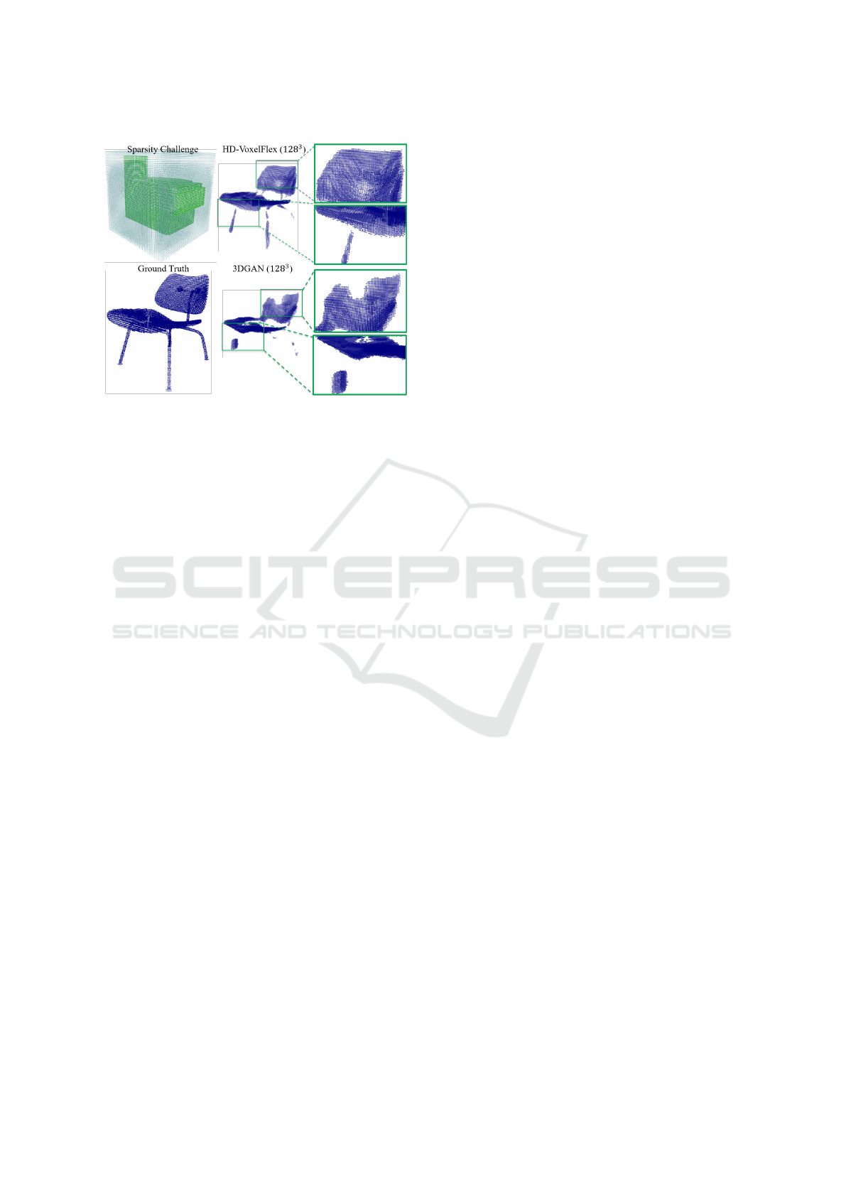
Figure 1: Top-Left: shows sparseness challenge given voxel

grid input and uneven distribution between full and empty

cells. Bottom-Left: “chair” model (ground truth) is en-

capsulated within a voxel grid of size 128

and is repre-

sented with 30,719 occupied cells (∼ 1.5% from the to-

tal number). Top-Right: reconstructed voxel grid through

HD-VoxelFlex. Bottom-Right: reconstructed voxel grid

through (Wu et al., 2015). Note: the number of unoccupied

cells is growing with the increase of the resolution; there-

fore, the sparseness challenge is increasing.

In our work, we propose a novel 3D CNN

encoder-decoder architecture that is able to build

effective representations from high-deﬁnition voxel

grid input with only moderate memory consumption.

To address the challenges associated with sparsity in

HD voxel grids, we introduce a set of building blocks

that include three architectural novelties: (1) random

shufﬂing to enhance the model’s generalization, (2)

skip connection to reduce information loss, (3) we in-

troduce kNN Distance Masks to enhance the accurate

modelling of local structure. In addition to these nov-

elties, we propose to use a combination of space-to-

depth layers and random shufﬂing to improve gener-

alization and to effectively reduce memory consump-

tion with only negligible effects on overall perfor-

mance. Moreover, we report on utilized literature-

based methods and their role in our training objec-

tives.

The speciﬁc contributions of this work are three-

fold. First, we present HD-VoxelFlex, the ﬁrst 3D

CNN encoder-decoder architecture that can be ap-

plied ﬂexibly to HD voxel grid inputs up to 192

with moderate memory consumption. Second, we

conduct comprehensive evaluations against the state-

of-the-art on different tasks: 3D reconstruction and

classiﬁcation. On ModelNet10/40 (Wu et al., 2015)

and PCN (Yuan et al., 2018) datasets, HD-VoxelFlex

outperforms the state-of-the-art in the reconstruction

task, while it outperforms/reaches competitive per-

formance in classiﬁcation on ModelNet10. Third,

we perform extensive ablation experiments to high-

light the signiﬁcance. Additionally, we document the

increase in memory usage compared to state-of-the-

art approaches, illustrating the efﬁcacy of the HD-

VoxelFlex.

2 RELATED WORK

In this work, we focus on the latent 3D data repre-

sentation given the voxel grid inputs since they ac-

curately preserve spatial relations. The reconstruc-

tion and classiﬁcation tasks reported in this work

provide insights into the effectiveness of the intro-

duced model and show that the model can be ap-

plied broadly. Categorization of 3D neural network

methodologies can be structured according to the type

of input data they utilize.; these are A) the raw data

(direct) point cloud approaches (Ran et al., 2022; Qi

et al., 2017a; Liao et al., 2018); B) Graph Convo-

lutions (Wang et al., 2019; Zhang et al., 2019) ap-

proaches, which incorporate local structure by con-

structing corresponding graphs; C) 2D Convolutions

methods on projections (Mescheder et al., 2019; Rad-

ford et al., 2015); and D) 3D Convolutions on voxel

grids (Schwarz et al., 2022; Liu et al., 2019; Riegler

et al., 2017). In the following, we will review each

type of approach.

Popular direct architectures are PointNet (Qi et al.,

2017a; Achlioptas et al., 2018), which assumes sim-

pliﬁed preprocessing. Yet, the proposed pooling oper-

ations result in a high information loss, where the re-

moval of shortcut connections does not work in prac-

tice either because of the utilization of global features

only (He et al., 2016; Ronneberger et al., 2015). An-

other disadvantage is the linear GPU consumption in

regard to the size of input. Therefore, the majority

of works handle PCD with ∼ 2K points unless down-

sampling techniques are applied. Note, the utilized

distance-based losses are ﬁt to sampling (Achlioptas

et al., 2017; Wang et al., 2020) instead of the objective

point PCD.

Another commonly adopted technique is based

on graph convolutions like Dynamic Graph CNN

(DGCNN) (Wang et al., 2019; Valsesia et al., 2018).

It works on raw PCD; however, in addition, it incor-

porates local geometric features to focus on neighbor-

hood details in speciﬁed areas through the introduced

Edge Convolution operations. The usage of pooling

layers, however, results in loss of information. More-

over, the creation of graphs consumes more resources

and additional time to process, respectively.

HD-VoxelFlex: Flexible High-Deﬁnition Voxel Grid Representation

205

Convolution on a 2D plane is another well-

researched paradigm. Besides, CNNs are applica-

ble in reconstruction and generative domains(Radford

et al., 2015) since they can follow a symmetric archi-

tecture, thus, resulting in balanced encoder and de-

coder parts. In CNNs, memory consumption depends

on the network depth rather than the input, and it is

sampling insensitive because of 2D images of a ﬁxed

resolution. However, due to applying 2D methods on

3D input, the information loss is the highest among

all reviewed approaches. Indeed, independent of the

viewpoint setup (Su et al., 2015), it is not possible to

universally represent the internal surfaces of the ob-

ject.

The remaining family of approaches reviewed in

this work is 3D convolutions on voxel grids. In ad-

dition to the advantages of 2D CNN, they do not cre-

ate any information loss. In contrast to raw input ap-

proaches, it is sampling insensitive and depends on

the voxel resolution or density, allowing small and

large PCDs to be handled together. The apparent dis-

advantage is the high memory utilization given low-

resolution inputs, an increased number of training pa-

rameters and high sparsity (the uneven ratio of ﬁlled

voxels to the total voxels in the grid). It has been con-

ﬁrmed through a set of recent works (Wu et al., 2017;

Wu et al., 2018; Zhang et al., 2018a) 3D convolutions

can be applied to resolutions up to 128

. However,

this is only possible with shallow architectures and

small batch sizes, which leads to slow training. Thus,

the aim of HD-VoxelFlex is to show effective voxel-

grid processing given various training objectives.

3 METHODOLOGY

Our overall architecture has an encoder-decoder

structure (see 2, inspired by VGG (Simonyan and Zis-

serman, 2014). To address the challenges resulting

from HD voxel grid data, we propose a set of novel

building blocks used in the network. We ﬁrst discuss

our speciﬁc techniques to address the aforementioned

challenges and subsequently explain how they are in-

tegrated into the networks’ building blocks.

3.1 Grouped Convolutions & Random

Shufﬂing

To reduce the overall number of training parameters,

we employ grouped convolutions (Krizhevsky et al.,

2017). Contrary to full convolutions (Krizhevsky

et al., 2017), where all input ﬁlters densely connect

to each output ﬁlter, with the total number of train-

ing parameters as k

∗ f

- stands for the kernel of

size x, features f = height ∗ width), a grouped convo-

lution is calculated within each group. Thus, it leads

to the parameters’ reduction, where the total number

of required weights is equal to k

∗ f

/g. Though g

is an additional hyperparameter and adjusts the total

number of weights, it is possible to regularize a net-

work by balancing the number of groups (Krizhevsky

et al., 2017), thus avoiding overﬁtting. Nonetheless,

the groups are isolated, where information ﬂow across

groups is limited. To propagate an isolated data ﬂow

along features/ﬁlters, a shufﬂe layer has been pro-

posed (Zhang et al., 2018b), allowing for information

ﬂow between the groups and provides additional regu-

larization without additional operations (Zhang et al.,

2018b). However, since the shufﬂe operations are

symmetrical, where f ( f (x)) = x, it leads to a permu-

tation loop; thus, due to the wide-most spread of in-

formation, the large networks might overﬁt and report

performance degradation. Instead of pre-determined

paths, we introduce a novel Random Shufﬂe (Fig-

ure 3, right) operation (initialized per model, in each

block), where paths and the information ﬂow is not

deterministic as in contrast to (Zhang et al., 2018b).

This decreases the probability of a permutation loop

to almost zero. Therefore, we utilize grouped convo-

lutions to reduce memory consumption and counter-

act the resulting isolation in information ﬂow with a

novel random shufﬂe operation.

3.2 3DVox Skip Connection

ResNet- (Ridnik et al., 2021; He et al., 2019; Bello

et al., 2021) and Inception-like works (Szegedy et al.,

2015; Szegedy et al., 2016; Szegedy et al., 2017) are

utilizing unit kernel convolutions (k

) to narrow the

network, whereas we exclude those, as they result in

signiﬁcant information loss (bottleneck). A represen-

tational bottleneck (Szegedy et al., 2016) refers to sig-

niﬁcant data compression occurrence at a designated

forward stage (cut). Therefore, to keep the entirety

of the information in the 3D reconstruction task, it is

paramount to avoid bottlenecks. Moreover, instead of

shortcut connections as in ResNet-D (He et al., 2019)

blocks and the average pooling operation, which cre-

ates a high information loss, we suggest a novel re-

ducing skip connection block 3DVox, which con-

sists of S2D projections, followed by batch normal-

ization, non-linearity and pointwise convolution (Fig-

ure 5, skip connections in projected shortcut blocks).

Such an approach yields no bottlenecks, with almost

no extra computations and is required to adjust the

resolution between the S2D layer and the main path.

Therefore, the spatial dimension is traded for the fea-

ture one. It is essential to note the difference to a

VISAPP 2024 - 19th International Conference on Computer Vision Theory and Applications

206

Figure 2: Visualization of our HD-VoxelFlex architecture (created with VisualKeras) for 64

inputs. Stem blocks for initial

dimensionality reduction are followed by shortcut and projected-shortcut blocks.

Figure 3: Middle: Shufﬂe operation as in line with Shuf-

ﬂeNet (Zhang et al., 2018b), where paths are algorithmi-

cally pre-deﬁned, sharing the information ﬂow between the

groups uniformly. Most right: proposed Random Shufﬂe

operation. Information ﬂow is shared non-uniformly, pro-

viding better regularization.

standard k

convolution, whereas in 3DVox the BN

layer aligns in both feature and spatial dimensions,

while k

projects in feature dimension only. There-

fore, it makes 3DVox more powerful in practice (see

Table 2).

3.3 Modelling Local Structure

Inspired by Graph Convolutions (Wang et al., 2019),

we propose to use a special layer to improve the mod-

elling of local structure in standard convolution lay-

ers. This is achieved using input masks as heatmaps,

where heat values incorporate local structure informa-

tion. We propose the usage of kNN-distance mask

(Figure 4) as heatmaps. To the best of our knowl-

edge, there are no prior works on utilizing kNN and

heatmap overall as an input, only as a weight mask

for loss optimization (Brock et al., 2016). We cal-

culate the heat values of the voxels as an average of

weights obtained from k neighbors, as in Equation 1.

A single weight w is squared inverse proportional to

the distance to the current neighbour (Equation 2).

h(v) =

∑

i∈1

w(v,v

)

(1)

w(v

) =

(1 + a ∗ d

)

(2)

Here, a denotes the decay rate and d the dis-

tance function (e.g. Euclidean metric). Alternative

masks, e.g., proportional, constant, variance and den-

sity heatmaps, are considered and summarized in Ta-

ble 4. The kNN distance mask tend to be more ef-

fective than other approaches (proportional or con-

stant masks, variance or density heatmaps), where,

according to our hypothesis, the distance-based pat-

tern is less evident for NN in contrast to the voxel-

based neighbourhood.

Figure 4: Sample of the kNN heatmap with neighbours=26

and decay rate=7 fused with voxel grid input (red points),

where in a training routine, we set neighbours=4, de-

cay rate=1.

3.4 Bag of Tricks

Based on a set of previous works listed further in this

section, we employ a number of important techniques

to improve performance and reduce memory require-

ments of HD-VoxelFlex.

Minimization of Pointwise Convolutions. In contra-

diction to (Szegedy et al., 2016), we minimized point-

wise (k

) convolutions to enlarge the receptive ﬁeld

HD-VoxelFlex: Flexible High-Deﬁnition Voxel Grid Representation

207

Figure 5: Proposed pre-activated building blocks. Skip connections are shown in projected shortcut building blocks of down-

sampling (in encoder, s2d → bn + act → k

s) and upsampling (in decoder, tr k

s → bn + act → d2s) modules.

Figure 6: Comparison of full (Krizhevsky et al., 2017),

grouped (Krizhevsky et al., 2017) and depthwise (Howard

et al., 2017) convolutions based on 3D VGG-like (Si-

monyan and Zisserman, 2014) architecture trained on Mod-

elNet10 for reconstruction task.

and introduce better generalization capabilities (Rid-

nik et al., 2021). As reported in (Ridnik et al., 2021),

the increase of receptive ﬁeld (utilization of k

ker-

nels) leads to reduced memory utilization. The ad-

ditional training parameters resulting from the larger

receptive ﬁelds are counteracted by grouped convo-

lutions (Krizhevsky et al., 2017) in pair with novel

random shufﬂing (see Section 3.1).

Minimization of Depthwise Convolutions. In con-

trast to previous works (Xie et al., 2017; Tan and Le,

2019; Howard et al., 2017), where authors claim that

the ﬁlter factorization leads to the model’s size be-

ing reduced, we refrain from using depthwise convo-

lutions (Howard et al., 2017), due to the ineffective

memory fragmentation as reported in (Ridnik et al.,

2021), resulting in poor GPU utilization. The numer-

ical assessments validating these assertions are in Fig-

ures 6, 7.

S2D/D2S Layers. We adopt another complementary

and effective method for reducing memory footprint,

known as a Space-to-Depth (S2D) layer (Shi et al.,

2016). The main advantage of S2D is the spatial and

subsequent feature-wise reduction of input maps, re-

Figure 7: Left: Coverage (higher better) metric compari-

son given different convolutions. Right: Minimum Match-

ing Distance (lower better) comparison given different con-

volutions. 3D VGG-like (Simonyan and Zisserman, 2014)

architecture trained on ModelNet10 used in reconstruction

task.

sulting in much lower memory consumption.

The S2D layer utilizes spatial correlation of its in-

put, making it effective at the early stages of the net-

work. On low-resolution input (i.e. at later stages),

inter-channel dependencies are stronger with no spa-

tial correlation.

An equivalent Symmetrical layer Depth-to-Space

(D2S) (Shi et al., 2016) is applied in Decoder, respec-

tively.

LeakyReLU. In contrast to the reported architectural

modiﬁcations as in (Sandler et al., 2018; Zhang et al.,

2018b), where linear activations instead of rectiﬁed

are applied, we propose to apply LeakyReLU, but

with a leak α

close to one. This larger leak value

counteracts the vanishing gradient problem that can

result from sparse activations resulting from sparse

HD voxel grid inputs.

In our experience, α

= 0.85 value leads to gra-

dient maximization without tedious and complex ar-

chitecture tuning, whereas 0.9 ≤ α

≤ 1.0 potentially

causes the lack of non-linearity and is, therefore, to be

avoided. Extended empirical evaluations in the form

of an ablation study, including model performance,

are reported in Table 3.

VISAPP 2024 - 19th International Conference on Computer Vision Theory and Applications

208

Squeeze-and-Excitation Block. SE (Hu et al., 2018)

block is used to improve feature inter-connection and

plays the role of a feature-wise attention mechanism

to compensate for grouped convolutions. Various ap-

plication of SE is in (Zhang et al., 2018b).

Stochastic Depth. In addition to the aforementioned

building blocks, we utilize Stochastic Depth (Huang

et al., 2016) with probability = 0.8 to drop a residual

path.

3.5 Proposed Blocks & Convolutional

Architecture

Incorporating the elements discussed above, we pro-

pose a set of convolutional building blocks (Fig-

ure 5) to build effective 3D representations. These

blocks are: A) stem - aiming for an effective initial

dimensionality reduction of the input; B) shortcut -

a none-strided residual block comparable to TRes-

Net (Ridnik et al., 2021); C) project shortcut - novel

strided residual block empowered with 3DVox skip

connection.

The effective input reduction in the stem block is

achieved with S2D operations, followed by a few k

to avoid aliasing. The shortcut is the main building

block and is represented by a set of pre-activated (He

et al., 2016) k

grouped convolutions and empow-

ered by our random shufﬂing layer for the channel

interaction. The projected shortcut block includes

3DVox skip connection to reduce data spatially. The

upsampling blocks in the decoder follow a symmetry

principle to the downsampling blocks. In stem up-

sampling block, the S2D operation is replaced with

a reversed Depth-to-Space (D2S) operation followed

by a few of k

pre-activated layers with the pur-

pose of smoothing and ﬁnal full-resolution activation.

The shortcut upsampling block completely coincides

with its downsampling counterpart, where convolu-

tions are replaced with a transposed version. The

primary modiﬁcation occurs within the upsampling

projection shortcut block, speciﬁcally along a resid-

ual path, where the initial convolutions involve s

, ad-

ditionally explained by antialiasing and the nature of

fractionally strided (transposed) convolution. The or-

der of layers (bn → act → trk

→ d

s) on the short-

cut path is not symmetrical to the downsample block.

According to our experimental ﬁndings, this sequence

proves to be more effective. The principle of pre-

activation could potentially elucidate this: the sub-

sequent neural layer’s input signal should comprise

neurons that have already been activated in the pre-

ceding layer. Furthermore, we support this arrange-

ment through ﬁlters’ pre-alignment, where the subse-

quent trk

computes image tiles with enhanced spa-

tial correlation.

In Figure 2, we render HD-VoxelFlex architecture,

but in 3D) composed of the described earlier blocks,

where the low-level resolution is handled differently

since our novel blocks are not effective for the sizes 2

and 4

because the padding in 3D takes a signiﬁcant

portion of the volume and ”dissolves” the signal. We

introduce a fully-convolutional structure and employ

a series of smaller kernel convolutions to minimize

the input signiﬁcantly. However, the ﬁnal convolution

equals a dense operation, particularly when the layer’s

local receptive ﬁeld matches the input size.

4 EVALUATIONS

Datasets. We utilize ModelNet-40 (Wu et al., 2015)

and its sliced version ModelNet-10 (Wu et al., 2015)

datasets for training and evaluation purposes. These

commonly adopted datasets contain a variety of ob-

jects with complex geometries, therefore, serve the

purposes of our research. Additionally, we employ

the PCN (Yuan et al., 2018) dataset, a benchmark

for the completion task, to conﬁrm the effectiveness

of HD-VoxelFlex. Due to a very sparse representa-

tion of the models (8 classes, in PCD) in PCN dataset,

we introduce (and make public) a new, voxel grid-

based PCN ground truth dataset, called VoxelPCN, in

128

and 192

resolutions. Besides, we make the en-

tire source code available, including the preprocess-

ing, dataset generation, and the framework for build-

ing 3D CNNs.

Preprocessing. PCD data itself is generated through

the random sampling of points from the CAD-

generated mesh’s triangular faces. Later, the data is

normalized to zero mean and embedded into a [-1,

1] bounding box, to preserve scale. The voxel grids

are formed from preprocessed point clouds, where

the voxel’s cell takes a ’full’ state if there is a point

in PCD at the corresponding location, ’empty’ other-

wise. Therefore, the level of detail depends on the

chosen voxel grid resolution under the assumption of

a high-density sampling step. Note, that while data

augmentation could be beneﬁcial, we leave it for fu-

ture work. Unlike ModelNet10/40 datasets, where

meshes are available, PCN dataset comes with an al-

ready predeﬁned set of sparse points preserving the

volumetric shape of each complete model with at

most 16384 points composed of 8 random FoV (par-

tial model representations). Therefore, the PCN sam-

pling step is omitted, involving only the normalization

and voxelization preprocessing stages.

Training Objective. In our work, we target the ge-

ometric completeness of the model given the recon-

HD-VoxelFlex: Flexible High-Deﬁnition Voxel Grid Representation

209

struction task by utilizing a voxel-based input (prob-

ability of the voxel cell being ﬁlled), which makes

the chosen evaluation metrics more precise. Hence,

we address the limitations associated with the eval-

uation methods of point cloud (Wang et al., 2019)

and statistics-based methods (Wu et al., 2016), where

points are better reconstructed at denser areas; points

are being reconstructed at areas of high conﬁdence,

respectively.

4.1 Metrics

The chosen metrics are split into four cate-

gories. The informational-based category includes

Binary-Cross Entropy (BCE) and Jensen-Shannon-

Divergence (JSD) metrics. The geometry-based cate-

gory includes Coverage and Minimum Matching Dis-

tance (MMD) metrics. The voxel-wise classiﬁca-

tion category of metrics, where we work with binary

classiﬁcation and measure Precision and Intersection-

over-Union (IoU) metrics. Lastly, the deep feature

supervised (SVM) and supervised classiﬁcation cate-

gory on latent codes of encoded images, which ad-

dresses the diversity of the proposed model. We as-

sume that each voxel is given as a binary random vari-

able; therefore, Jensen-Shannon Divergence is formu-

lated as in Equation 3.

JSD(P

||P

) =

D(P

||M) +

D(P

||M) (3)

where M is the average value between predictions

and is given as M =

+ P

). D(X||Y ) stands for

Kullback-Leibler Divergence between distributions X

and Y , i.e. amount of information loss.

The Coverage and MMD are calculated based on

Chamfer Distance given in Equation 4

(S1,S2) =

∑

x∈S

min

y∈S

||x − y||

∑

y∈S

min

x∈S

||x − y||

(4)

Therefore, for each reconstructed point

,...,y

||S

} ∈ S

, there exists a set of

nearest neighbors in the original set N =

,...,x

||S

} ∈ S

. Chamfer Distance mea-

sures the minimum distance from each point of both

point sets to the corresponding nearest neighbors.

The Coverage is the ratio of unique points in N over

cardinality of S1 as is formulated in Equation 5.

Coverage(S2,S1) =

|||unique(N)||

||S

∗ 100% (5)

MMD distance stands for the average distance to the

covered points from the reconstructed point cloud.

Therefore, is the 2nd term of the Chamfer Distance

averaged with the cardinality of the reconstructed

point set as is formulated in Equation 6.

MMD(S2,S1) =

∑

||S

i=0

||N

− S

||S

(6)

Precision and IoU are calculated similarly to the

binary classiﬁcation problem with the binary out-

come in the reconstruction of voxel grids as V

True

i, j,k

Reconstructed

j, j,k

. Therefore, it gives four possible out-

comes T P, TN, FP, FN. In practice, precision mea-

sures how exact the reconstruction is. Coverage

stands for the reconstruction of the volumetric sur-

face, where MMD measures how well-reconstructed

the surface is. Lastly, IoU reports how much common

surface the two models have relative to the overall sur-

face.

Table 1: Ablation study to emphasize the gain of the chosen

methods and introduced novelties.

Utilized bag of methods (tricks) Cov., %

ResnetD block

(He et al., 2019) +21.17

Grouped Convolutions (GC)

(Krizhevsky et al., 2017) (Section 3) +0.06

Decrease Pointwise/Increase GC

(He et al., 2019) (Sect. 3) +7.31

Groups everywhere / Shufﬂing +0.78

No Pointwise Conv. (PwC)

(Ridnik et al., 2021) (Section 3) +1.3

Space-to-Depth (S2D)

(Shi et al., 2016) (Section 3) -0.46

Zero padding +0.12

Stochastic Depth

(Huang et al., 2016) +2.09

Label Smoothing

(Szegedy et al., 2016) +0.64

SE Blocks

(Hu et al., 2018) +0.16

Leaky ReLU = 0.85 (Section 3.4) +5.32

Our novelties

Random Shufﬂing (Section 3.1) +0.57

3DVox Skip Connections (Sect. 3) +2.02

kNN Distance Masking (Section 3.3) +2.6

Table 2: Evaluation of reducing skip-connections.

Approach BCE Coverage MMD

No projected

shortcuts(baseline)

0.0610 81.09 0.0085

Pooling + k1s1(SOTA) 0.0611 81.65 0.0082

Concatenation

(Zhang et al., 2018b) 0.0779 81.47 0.0084

S2D + k1s1 (3DVox) 0.0681 83.11 0.0074

VISAPP 2024 - 19th International Conference on Computer Vision Theory and Applications

210

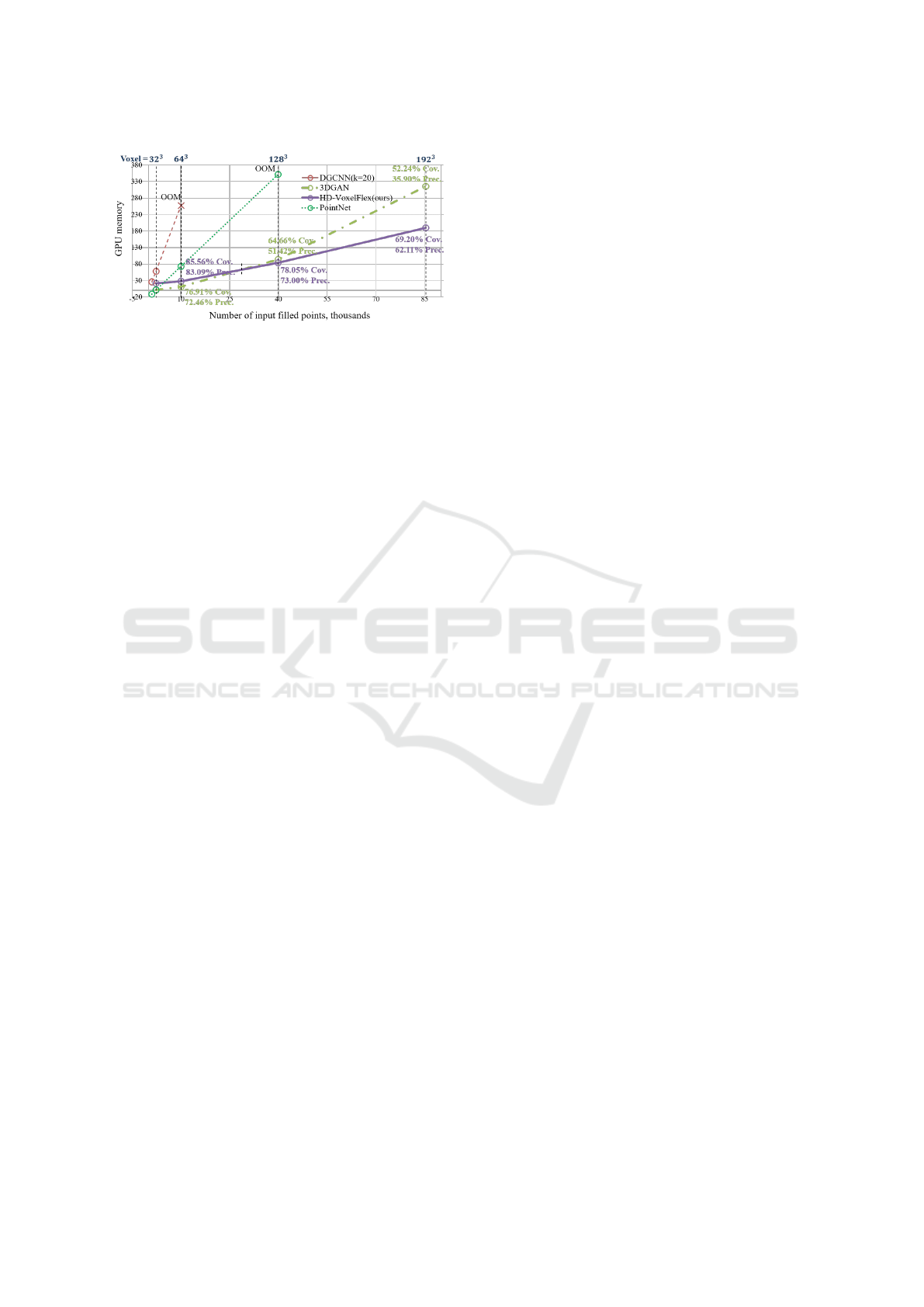
Figure 8: HD-VoxelFlex shows a minor increase in mem-

ory utilization with a signiﬁcant input size increase (from

2.3K → 10K → 40K → 85K, where points are averaged),

while preserving the best performance despite signiﬁcant

data sparsity.

4.2 Quantitative Evaluations

We perform various evaluations given low-resolution

/64

and high-resolution 128

/192

voxel grid se-

tups. The number of occupied voxel grid cells (see

Figure 8) as the sparseness ratio increases with the

increase of voxel grid resolution. The models in

PCN (Yuan et al., 2018) dataset are always described

with a ﬁxed number of points (16384). Thus, we in-

troduce a voxel-based version of PCN dataset.

As shown in Table 5, given the lower/higher def-

inition input, HD-VoxelFlex models (with and with-

out the mask) demonstrate state-of-the-art results in

reconstruction. The overall drop in performance is

driven by the increased data sparsity as the result of

enlarging voxel grid resolution. 3D-GAN shows plau-

sible results. Segmentation models with low resolu-

tion have shown good results; however, the utiliza-

tion of shortcut connections makes them unusable for

our purposes. Notably, our models are much better

on coverage while still demonstrating performance on

classiﬁcation (Table 6), which is on par with the state-

of-the-art.

4.3 Qualitative Evaluations

Qualitative evaluations are shown in Figures 9. For a

lower deﬁnition voxel grid (32

/64

), we’ve obtained

close to 100% coverage for simple shapes, whereas

for more complex shapes, coverage dropped to ∼90-

93% (samples of ﬁgures with associated metrics are

on Figures 10 and 11, with their corresponding met-

rics provided in Tables 7 and 8, respectively). For

the higher deﬁnition voxel grid (128

), renderings

conﬁrm a drop in performance caused by increased

sparsity and the underlying complexity of input (Fig-

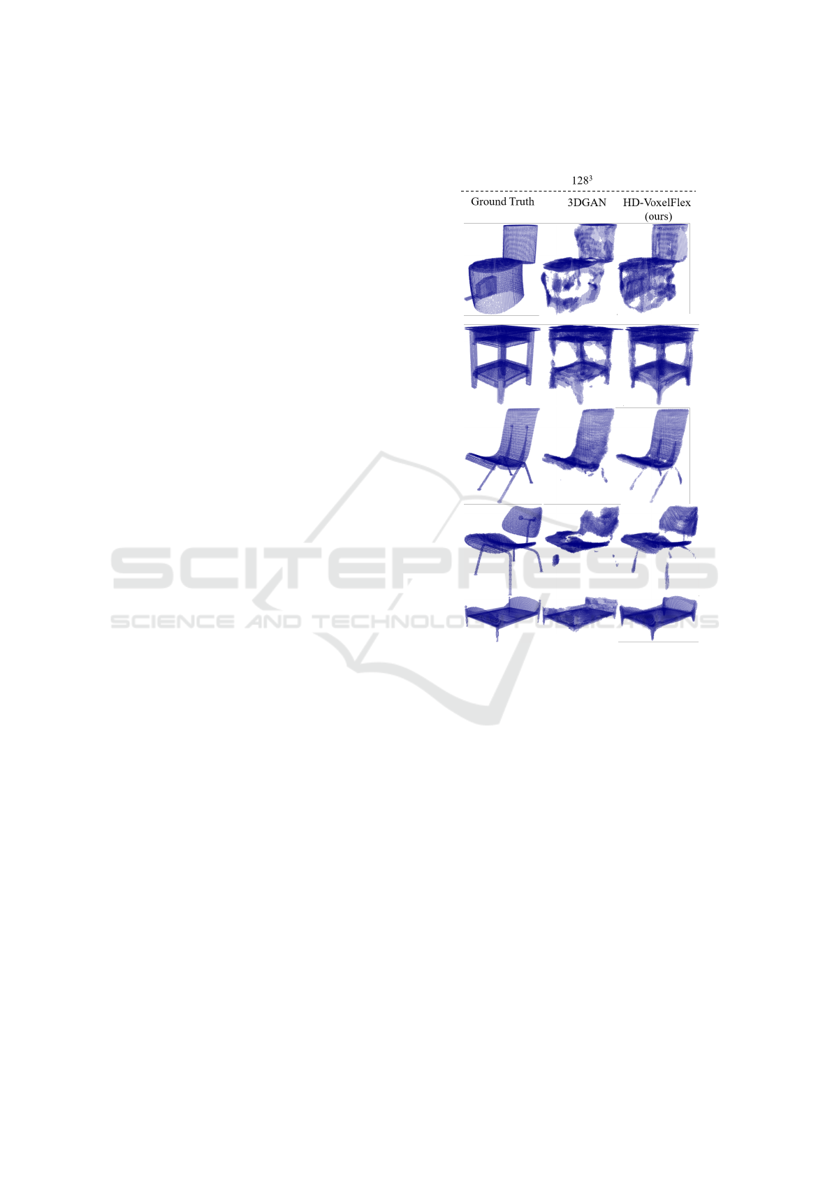
ures 12, and 13, in Appendix).

4.4 Ablation and Memory Evaluations

In Table 1, we report the gain (Coverage in % re-

garding the overall performance of the baseline VGG-

3D (Simonyan and Zisserman, 2014)) of the selected

methods. Moreover, we list the gain of introduced

novelties. Importantly, as depicted in Figure 8, we

report GPU usage, where point cloud-based meth-

ods consume more vGPU than convolutional, whereas

GraphConv.-based methods (10k of points, 64

) have

run into memory overﬂow. 3DGAN network con-

sumes less memory than HD-VoxelFlex in lower res-

olution setups; however, we empirically demonstrate

almost linear growth in memory utilization with the

resolution increase. 3DGAN, on the other hand,

demonstrates a drastic increase in memory usage.

This proves our research objective that HD-VoxelFlex

effectively represents high-deﬁnition voxel grid in-

puts despite sparsity and memory utilization chal-

lenges.

An additional input (a heatmap), also referred to

as a mask, is considered. Various input masks were

tested in experiments and reported as ablation study in

Table 4. A proportional mask, where the heat values

encode a ratio between full and empty voxels. There-

fore, the proportional masks are mainly considered in

sparse voxel grids and is to be considered in future

work in higher-resolution setups with further evalua-

tions related to PCN and/or Completion3D datasets.

Yet, in setups with 64

no signiﬁcant improvements

were indicated, which is potentially justiﬁed by the

ability of HD-VoxelFlex to recover the ratio between

empty and full cells. A constant mask, stands for

a more generalized version of a proportional mask,

where the heat values are assigned a pre-deﬁned

pair of constants. No signiﬁcant improvements were

shown in the course of the ablation 4 study either. The

construction of a variance heatmap relies on calcu-

lating the variance within a designated receptive win-

dow, where the entirely empty or full windows, are

being assigned with null variance. Therefore, it is

meant to empower the reconstruction of the border re-

gions of the model, where improvements were shown

in comparison to previous ones. The concept of the

density heatmap drew inspiration from the classical

Minesweeper game, where the heat value is indicative

of how many ﬁlled voxels (mines) are adjacent to the

current voxel. The shown performance is compara-

ble to the early introduced variance heatmap. The ap-

proach suggested in this work, k-Nearest Neighbors

Distance (kNN) input mask, is the most reﬁned tech-

nique in comparison to previously listed ones. Ad-

ditionally, its performance was conﬁrmed by the re-

ported ablation study. The heat values are estimated

HD-VoxelFlex: Flexible High-Deﬁnition Voxel Grid Representation

211

Table 3: Ablation evaluation of activation functions on VGG-like 3D architecture. LeakyReLU with the leak value set to 0.85

empirically shown the best performance.

Activation BCE Coverage MMD

LeakyReLU (0.1) 0.0922 80.59 0.5342

LeakyReLU (0.3) 0.785 80.76 0.5485

LeakyReLU (0.85) 0.0669 83.72 0.5407

LeakyReLU (1.2) 0.0688 83.15 0.5031

ReLU 0.0812 79.86 0.5187

Hard sigmoid (Courbariaux et al., 2015) 0.0878 77.87 0.5711

Sigmoid 0.0893 77.08 0.5895

PReLU (0.85) (He et al., 2015) 0.0688 83.28 0.5464

cw-PReLU (0.85) 0.0677 83.09 0.5428

Swish (β = 1) (Ramachandran et al., 2017) 0.0838 79.52 0.5457

Swish (β = 0.05) 0.0878 81.23 0.6320

Swish (β = 1) 0.0864 78.74 0.5581

SELU (Klambauer et al., 2017) 0.0827 81.44 0.5470

rReLU(-1.5, 1.4, 0.85, 1.4, 1.5) 0.0754 82.79 0.5571

rReLU(-2.5, 0.2, 0.7, 0.2, 2.5) 0.0766 81.82 0.5012

Table 4: Ablation report for different masking methods for 64

voxel grid setup. Note that a set of evaluations is yet to be

conducted in future for higher-resolution voxel-grid setups, considering the proportional mask and its beneﬁts. Moreover, a

combination of numerous masks is also planned, aiming to combine the beneﬁts of each individual method. However, an

expensive ﬁne-tuning is to be assumed.

Description Coverage, % MMD Precision, %

No mask applied (baseline) 85,56% 5,59E-03 83,09%

Constant weighed mask (gamma=0.97) 75,49% 1,07E-02 67,40%

Constant weighed mask (gamma=0.97); voxels normalization 80,18% 7,98E-03 74,89%

Proportional weighed mask 80,07% 8,17E-03 75,28%

Proportional weighed mask; unit normalization 80,74% 7,58E-03 76,48%

Proportional weighed mask; voxels normalization 78,83% 8,39E-03 73,65%

Variance area=1 84,77% 7,11E-03 82,45%

Variance area=1; ls=0.05 84,76% 7,05E-03 82,40%

Variance area=1; ls=0.0 82,71% 9,02E-03 80,02%

Variance area=3; ls=0.05 84,08% 1,25E-02 81,48%

Variance area=1; ls=0.26; voxels normalization 84,95% 6,90E-03 82,48%

Variance area=3; ls=0.26; voxels normalization 84,19% 9,65E-03 81,87%

Density area=3; intensity=(1, 1); ls=0.05 82,25% 1,95E-02 79,21%

Density area=3; intensity=(1, 1); ls=0.26; voxel normalization 82,77% 2,32E-02 79,75%

Density area=1; intensity=(3, 1); 84,89% 7,04E-03 82,43%

Density area=1; intensity=(5, 1); 84,41% 7,27E-03 82,04%

Density area=2; intensity=(5, 1); 83,60% 1,44E-02 80,92%

KNN k=1; a=4 88,16% 4,43E-03 86,55%

KNN k=1; a=7 88,04% 4,52E-03 85,71%

KNN k=8; a=7 84,44% 6,02E-03 81,27%

KNN k=26; a=7 88,11% 4,44E-03 86,41%

based on distances from the current voxel to its k-

nearest ﬁlled neighbours, with a ﬁxed decay rate. A

moderate set of parameters is to be chosen to avoid

overﬁtting. To resume, the kNN distance input mask

proved its effectiveness and is reported in Table 4.

5 DISCUSSION, FUTURE WORK

In-place activated batch normalization (Bulo et al.,

2018) approach is considered a reasonable way to

reduce GPU usage since no additional memory is

needed for backpropagation. Instead, an update to

the weights is calculated on the ﬂy from an output

VISAPP 2024 - 19th International Conference on Computer Vision Theory and Applications

212

Table 5: Numerical evaluations given ModelNet10 (Wu et al., 2015) and PCN (Yuan et al., 2018) datasets in various reso-

lutions. PCN dataset is much sparser due to the absence of a sampling step as we work directly with predeﬁned point cloud

data, which causes a signiﬁcant drop in evaluation metrics.

Architecture Res.

Reconstruction

BCE JSD Coverage, % MMD Precision, % IoU, %

3DGAN (Wu et al., 2016)

128

192

0.4317

0.4084

0.4053

0.4000

3.95E-05

2.74E-06

4.40e-08

4.81e-09

74.75

76.91

64.66

52.24

0.0234

0.0107

0.0144

0.0185

69.73

72.46

51.42

35.90

53.53

56.81

34.61

21.88

PointNet (Qi et al., 2017a)

- -

90.57

73.48

0.0087

0.0674

86.11

59.5

43.93

35.38

PointNetAE (Qi et al., 2017a; Achlioptas

et al., 2017)

- -

39.81

27.65

0.0557

0.1292

17.46

14.33

7.02

4.25

DGCNN (Wang et al., 2019) 32

- -

89.72 0.0093 85.26 47.96

DGCNNAE (Wang et al., 2019; Achliop-

tas et al., 2017)

- -

52.08 0.0429 22.71 9.08

HD-VoxelFlex (ours)

128

192

0.3934

0.4004

0.3970

0.3956

5.76E-06

1.30E-06

2.42e-08

6.49e-09

96.11

85.56

78.05

69.20

0.0025

0.0056

0.0055

0.0072

95.81

83.09

73.00

62.11

91.96

71.08

57.48

45.04

HD-VoxelFlex Mask (ours)

0.3947

0.3979

1.86E-05

1.11E-06

96.24

88.16

0.0025

0.0044

95.89

86.55

92.11

76.30

HD-VoxelFlex (PCN (Yuan et al., 2018)

dataset)

128

0.3913 1.35e-08 50.18 0.0104 38.88 24.13

Table 6: The numerical evaluations for lowerer deﬁnition voxel grids (32

) with ∼ 2K of points and (64

) with ∼ 10K of

points, respectively. HD-VoxelFlex shows comparable to the state-of-the-art results in the classiﬁcation task, where given

ModelNet10 (Wu et al., 2015) dataset, we outperform SOTA models in the supervised classiﬁcation.

Resolution=32

/64

Deep Feature

Classiﬁcation, %

Supervised Classiﬁcation, %

Architecture SVM MN10 MN40

3DGAN (Wu et al., 2016) 87.61 / 89.29 90.35 / 90.95 84.58 / 84.42

PointNet (Qi et al., 2017a) 74.44 / 72.21 91.51 / 90.90 87.70 / 88.32

PointNetAE (Qi et al., 2017a; Achlioptas et al., 2017) 22.32 / 13.73 - -

DGCNN (Wang et al., 2019) 69.53 / - 91.95 / - 91.50 / -

DGCNNAE (Wang et al., 2019; Achlioptas et al., 2017) 11.27 / - - -

VoxelFlex (ours) 84.71

3rd

/88.06

2nd

90.90/91.89 86.92/86.43

VoxelFlex (ours with mask) 87.39

2nd

/85.49 91.60

2nd

/92.25 87.23

3rd

/86.73

2nd

Figure 9: Qualitative renderings of random samples with different geometry and level of detail complexity. HD-VoxelFlex

demonstrates the best performance, including complex inputs and higher resolutions 128

. While the direct approaches (with

sufﬁx AE), due to the lack of local features, demonstrate the lowest. In 64

setup, the overall performance is lower than 32

due to the increased data sparsity. The same holds in relation to 128

. DGCNN and DGCNNAE results are not shown in 64

resolution due to insufﬁcient vGPU memory. PointNetAE in 64

is removed because of the poor performance. We provide

a sample from PCN dataset in 128

, where HD-VoxelFlex tends to recover a more structural (grid-based) representation

(targeted intention).

HD-VoxelFlex: Flexible High-Deﬁnition Voxel Grid Representation

213

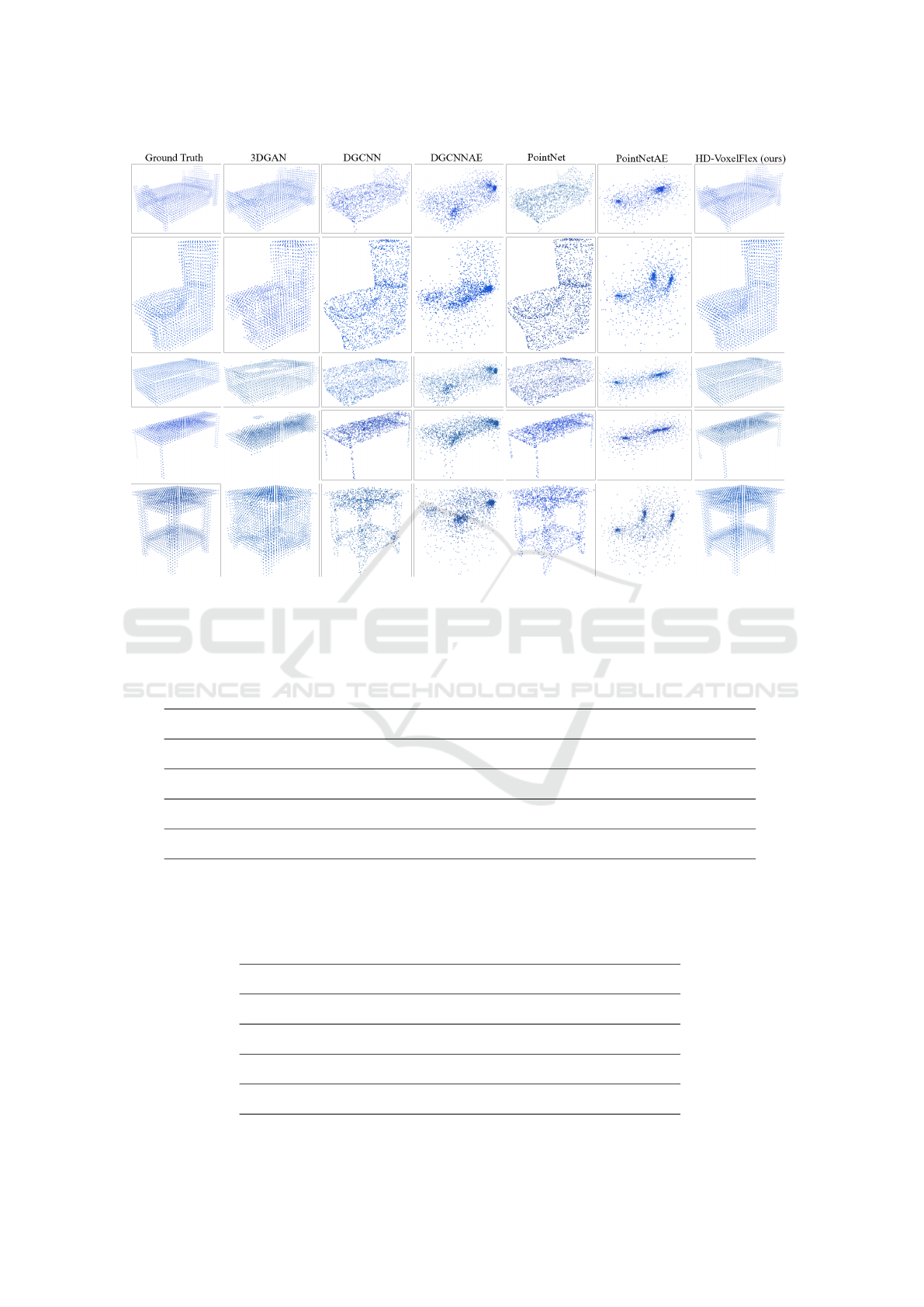
Figure 10: The qualitative renderings of 32

or ∼ 2.3K (in the setups with raw point cloud data input) points with different

geometrical complexity. The introduced HD-VoxelFlex shows the best performance, including complex models. While the

direct approaches (with sufﬁx AE), due to the lack of local features, demonstrate the lowest. The afﬁliated sampled-based

performance is listed in Table 7.

Table 7: Coverage and MMD numerical evaluations, which correspond to the 32

voxel grid qualitative renderings plotted in

Figure 10. In all randomly provided samples, the HD-VoxelFlex approach demonstrates the best performance.

Ground Truth 3DGAN DGCNN DGCNNAE PointNet PointNetAE VoxelFlex (ours)

Coverage = 100% 84,26% 90,11% 58,84% 88,78% 39,55% 95,76%

MMD = 0 1,17E-02 1,57E-02 5,95E-02 1,71E-02 8,21E-02 2,71E-03

Coverage = 100% 73,32% 85,90% 47,82% 91,98% 39,88% 95,01%

MMD = 0 2,18E-02 1,33E-02 6,61E-02 6,83E-03 8,47E-02 3,27E-03

Coverage = 100% 85,82% 94,73% 59,32% 93,99% 40,61% 98,99%

MMD = 0 1,06E-02 5,79E-03 9,15E-02 7,19E-03 1,38E-01 6,31E-04

Coverage = 100% 75,99% 95,83% 50,77% 93,06% 48,53% 98,53%

MMD = 0 1,85E-02 4,69E-03 6,68E-02 5,41E-03 7,62E-02 1,05E-03

Coverage = 100% 68,86% 88,03% 39,59% 91,33% 26,20% 97,25%

MMD = 0 3,91E-02 1,22E-02 9,56E-02 6,93E-03 1,59E-01 1,74E-03

Table 8: Coverage and MMD numerical evaluations, which correspond to the 64

voxel grid qualitative renderings plotted

in Figure 11. Note that despite a better-shown performance of PointNet in Coverage (bottom sample), the MMD result

still conﬁrms that our approach is better in ﬁne-grained reconstruction. In the remaining random samples, our approach

demonstrates the best performance.

Ground Truth 3DGAN PointNet PointNetAE VoxelFlex (ours)

Coverage = 100% 91,88% 88,05% 0,53% 93,91%

MMD = 0 9,48E-03 1,08E-02 5,70E-01 2,71E-03

Coverage = 100% 77,63% 90,36% 55,94% 90,80%

MMD = 0 1,54E-02 6,46E-03 6,88E-02 4,56E-03

Coverage = 100% 91,19% 94,77% 1,06% 97,29%

MMD = 0 6,54E-03 8,61E-03 6,98E-01 8,72E-04

Coverage = 100% 87,97% 63,84% 64,58% 96,06%

MMD = 0 1,10E-02 2,80E-02 5,86E-02 4,57E-03

Coverage = 100% 86,34% 94,59% 48,18% 91,54%

MMD = 0 1,03E-02 5,33E-03 7,38E-02 2,70E-03

VISAPP 2024 - 19th International Conference on Computer Vision Theory and Applications

214

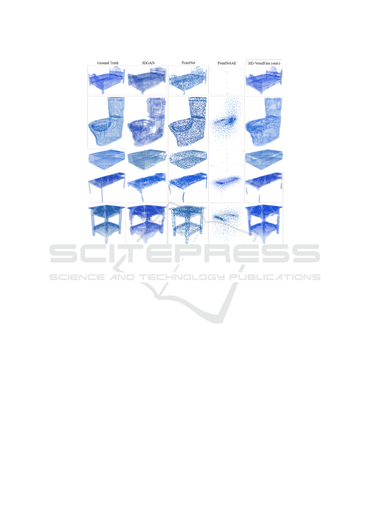
Figure 11: The qualitative renderings of 64

or ∼ 10K (in the setups with raw point cloud data) points with different geo-

metrical complexity. The introduced HD-VoxelFlex shows the best performance, including complex models. While the direct

approaches (with sufﬁx AE), due to the lack of local features, demonstrate the lowest. DGCNN and DGCNNAE results are

not shown due to out-of-memory errors. The afﬁliated sampled-based performance is listed in Table 8.

map after activation (increased voxel grid, but slower

training routine). Besides, potentially, the biggest

drawback for 3D convolutions is the sparsity of input.

Therefore, Sparse Convolutions (Yan et al., 2018) can

be tested, where multiplications are dependent on a

special scheduling rule book, which addresses non-

zero voxels and their multiplications. Hence, this

potentially makes HD-VoxelFlex applicable to large

indoor/outdoor scenes. Followed by an additional

comparative study to sparse voxel-based (Zhao et al.,

2022) input methods. Furthermore, it is interesting

to incorporate HD-VoxelFlex with Neural Radiance

Fields (Mildenhall et al., 2020) (NRF) to improve the

overall reconstruction performance. Moreover, Gaus-

sian Mixture Models (GMM) (Achlioptas et al., 2018)

has proven its effectiveness for synthesizing unseen

models; therefore, it is yet a question to explore.

6 CONCLUSION

This work addresses high-deﬁnition voxel grid rep-

resentation inputs by proposing a novel 3D CNN ar-

chitecture called HD-VoxelFlex. Despite the sparsity

and high-memory utilization challenges, we show that

3D CNN on voxel grid inputs are more reasonable for

3D representation, where HD-VoxelFlex can handle

higher deﬁnition input without compromising mem-

ory utilization. Importantly, a set of improvements

were suggested, like novel random shufﬂing, reduced

skip connection, a set of novel building blocks, and

kNN distance mask fuse, forming an improved ar-

chitecture and resulting in state-of-the-art results in

reconstruction. Besides, our model demonstrated re-

sults on the level with the SOTA in classiﬁcation.

ACKNOWLEDGEMENTS

This work has been funded by the German Ministry

for Research and Education (BMBF) in the project

MOMENTUM (grant number 01IW22001) and open-

SCENE (Software Campus program) project.

P. M

uller was funded by the European Union

Horizon Europe program (grant number 101078950).

HD-VoxelFlex: Flexible High-Deﬁnition Voxel Grid Representation

215

REFERENCES

Achlioptas, P., Diamanti, O., Mitliagkas, I., and Guibas,

L. (2017). Representation learning and adversar-

ial generation of 3d point clouds. arXiv preprint

arXiv:1707.02392, 2(3):4.

Achlioptas, P., Diamanti, O., Mitliagkas, I., and Guibas, L.

(2018). Learning representations and generative mod-

els for 3d point clouds. In International conference on

machine learning, pages 40–49. PMLR.

Bello, I., Fedus, W., Du, X., Cubuk, E. D., Srinivas, A.,

Lin, T.-Y., Shlens, J., and Zoph, B. (2021). Revisit-

ing resnets: Improved training and scaling strategies.

Advances in Neural Information Processing Systems,

34:22614–22627.

Boulch, A. and Marlet, R. (2022). Poco: Point convolu-

tion for surface reconstruction. In Proceedings of the

IEEE/CVF Conference on Computer Vision and Pat-

tern Recognition, pages 6302–6314.

Brock, A., Lim, T., Ritchie, J. M., and Weston, N.

(2016). Generative and discriminative voxel modeling

with convolutional neural networks. arXiv preprint

arXiv:1608.04236.

Bulo, S. R., Porzi, L., and Kontschieder, P. (2018). In-place

activated batchnorm for memory-optimized training

of dnns. In Proceedings of the IEEE Conference

on Computer Vision and Pattern Recognition, pages

5639–5647.

Courbariaux, M., Bengio, Y., and David, J.-P. (2015). Bina-

ryconnect: Training deep neural networks with binary

weights during propagations. Advances in neural in-

formation processing systems, 28.

Hatamizadeh, A., Tang, Y., Nath, V., Yang, D., Myronenko,

A., Landman, B., Roth, H. R., and Xu, D. (2022). Un-

etr: Transformers for 3d medical image segmentation.

In Proceedings of the IEEE/CVF winter conference on

applications of computer vision, pages 574–584.

He, K., Zhang, X., Ren, S., and Sun, J. (2015). Delv-

ing deep into rectiﬁers: Surpassing human-level per-

formance on imagenet classiﬁcation. In Proceedings

of the IEEE international conference on computer vi-

sion, pages 1026–1034.

He, K., Zhang, X., Ren, S., and Sun, J. (2016). Deep resid-

ual learning for image recognition. In Proceedings of

the IEEE conference on computer vision and pattern

recognition, pages 770–778.

He, T., Zhang, Z., Zhang, H., Zhang, Z., Xie, J., and Li,

M. (2019). Bag of tricks for image classiﬁcation with

convolutional neural networks. In Proceedings of the

IEEE/CVF conference on computer vision and pattern

recognition, pages 558–567.

Howard, A. G., Zhu, M., Chen, B., Kalenichenko, D.,

Wang, W., Weyand, T., Andreetto, M., and Adam,

H. (2017). Mobilenets: Efﬁcient convolutional neu-

ral networks for mobile vision applications. arXiv

preprint arXiv:1704.04861.

Hu, J., Shen, L., and Sun, G. (2018). Squeeze-and-

excitation networks. In Proceedings of the IEEE con-

ference on computer vision and pattern recognition,

pages 7132–7141.

Huang, G., Sun, Y., Liu, Z., Sedra, D., and Weinberger,

K. Q. (2016). Deep networks with stochastic depth. In

Computer Vision–ECCV 2016: 14th European Con-

ference, Amsterdam, The Netherlands, October 11–

14, 2016, Proceedings, Part IV 14, pages 646–661.

Springer.

Klambauer, G., Unterthiner, T., Mayr, A., and Hochreiter, S.

(2017). Self-normalizing neural networks. Advances

in neural information processing systems, 30.

Krizhevsky, A., Sutskever, I., and Hinton, G. E. (2017). Im-

agenet classiﬁcation with deep convolutional neural

networks. Communications of the ACM, 60(6):84–90.

Li, W., Wang, G., Fidon, L., Ourselin, S., Cardoso, M. J.,

and Vercauteren, T. (2017). On the compactness, ef-

ﬁciency, and representation of 3d convolutional net-

works: brain parcellation as a pretext task. In Infor-

mation Processing in Medical Imaging: 25th Inter-

national Conference, IPMI 2017, Boone, NC, USA,

June 25-30, 2017, Proceedings 25, pages 348–360.

Springer.

Li, Z., Gao, P., Yuan, H., Wei, R., and Paul, M. (2023).

Exploiting inductive bias in transformer for point

cloud classiﬁcation and segmentation. arXiv preprint

arXiv:2304.14124.

Liao, Y., Donne, S., and Geiger, A. (2018). Deep march-

ing cubes: Learning explicit surface representations.

In Proceedings of the IEEE Conference on Computer

Vision and Pattern Recognition, pages 2916–2925.

Liu, Z., Tang, H., Lin, Y., and Han, S. (2019). Point-voxel

cnn for efﬁcient 3d deep learning. Advances in Neural

Information Processing Systems, 32.

Mescheder, L., Oechsle, M., Niemeyer, M., Nowozin, S.,

and Geiger, A. (2019). Occupancy networks: Learn-

ing 3d reconstruction in function space. In Proceed-

ings of the IEEE/CVF conference on computer vision

and pattern recognition, pages 4460–4470.

Mi, Z., Di, C., and Xu, D. (2022). Generalized binary search

network for highly-efﬁcient multi-view stereo. In Pro-

ceedings of the IEEE/CVF Conference on Computer

Vision and Pattern Recognition, pages 12991–13000.

Mildenhall, B., Srinivasan, P. P., Tancik, M., Barron, J. T.,

Ramamoorthi, R., and Ng, R. (2020). Nerf: Repre-

senting scenes as neural radiance ﬁelds for view syn-

thesis. In ECCV.

Oleksiienko, I. and Iosiﬁdis, A. (2021). Analysis of voxel-

based 3d object detection methods efﬁciency for real-

time embedded systems. In 2021 International Con-

ference on Emerging Techniques in Computational In-

telligence (ICETCI), pages 59–64. IEEE.

Phan, A. V., Le Nguyen, M., Nguyen, Y. L. H., and Bui,

L. T. (2018). Dgcnn: A convolutional neural network

over large-scale labeled graphs. Neural Networks,

108:533–543.

Qi, C. R., Su, H., Mo, K., and Guibas, L. J. (2017a). Point-

net: Deep learning on point sets for 3d classiﬁcation

and segmentation. In Proceedings of the IEEE con-

ference on computer vision and pattern recognition,

pages 652–660.

Qi, C. R., Yi, L., Su, H., and Guibas, L. J. (2017b). Point-

net++: Deep hierarchical feature learning on point sets

in a metric space. Advances in neural information pro-

cessing systems, 30.

VISAPP 2024 - 19th International Conference on Computer Vision Theory and Applications

216

Radford, A., Metz, L., and Chintala, S. (2015). Unsu-

pervised representation learning with deep convolu-

tional generative adversarial networks. arXiv preprint

arXiv:1511.06434.

Ramachandran, P., Zoph, B., and Le, Q. V. (2017).

Searching for activation functions. arXiv preprint

arXiv:1710.05941.

Ran, H., Liu, J., and Wang, C. (2022). Surface representa-

tion for point clouds. In Proceedings of the IEEE/CVF

Conference on Computer Vision and Pattern Recogni-

tion, pages 18942–18952.

Ridnik, T., Lawen, H., Noy, A., Ben Baruch, E., Sharir,

G., and Friedman, I. (2021). Tresnet: High perfor-

mance gpu-dedicated architecture. In proceedings of

the IEEE/CVF winter conference on applications of

computer vision, pages 1400–1409.

Riegler, G., Osman Ulusoy, A., and Geiger, A. (2017). Oct-

net: Learning deep 3d representations at high reso-

lutions. In Proceedings of the IEEE conference on

computer vision and pattern recognition, pages 3577–

3586.

Ronneberger, O., Fischer, P., and Brox, T. (2015). U-

net: Convolutional networks for biomedical image

segmentation. In Medical Image Computing and

Computer-Assisted Intervention–MICCAI 2015: 18th

International Conference, Munich, Germany, October

5-9, 2015, Proceedings, Part III 18, pages 234–241.

Springer.

Sandler, M., Howard, A., Zhu, M., Zhmoginov, A., and

Chen, L.-C. (2018). Mobilenetv2: Inverted residu-

als and linear bottlenecks. In Proceedings of the IEEE

conference on computer vision and pattern recogni-

tion, pages 4510–4520.

Schwarz, K., Sauer, A., Niemeyer, M., Liao, Y., and

Geiger, A. (2022). Voxgraf: Fast 3d-aware image

synthesis with sparse voxel grids. arXiv preprint

arXiv:2206.07695.

Shi, W., Caballero, J., Husz

ar, F., Totz, J., Aitken, A. P.,

Bishop, R., Rueckert, D., and Wang, Z. (2016). Real-

time single image and video super-resolution using an

efﬁcient sub-pixel convolutional neural network. In

Proceedings of the IEEE conference on computer vi-

sion and pattern recognition, pages 1874–1883.

Simonyan, K. and Zisserman, A. (2014). Very deep con-

volutional networks for large-scale image recognition.

arXiv preprint arXiv:1409.1556.

Su, H., Maji, S., Kalogerakis, E., and Learned-Miller, E.

(2015). Multi-view convolutional neural networks for

3d shape recognition. In Proceedings of the IEEE

international conference on computer vision, pages

945–953.

Szegedy, C., Ioffe, S., Vanhoucke, V., and Alemi, A. (2017).

Inception-v4, inception-resnet and the impact of resid-

ual connections on learning. In Proceedings of the

AAAI conference on artiﬁcial intelligence, volume 31.

Szegedy, C., Liu, W., Jia, Y., Sermanet, P., Reed, S.,

Anguelov, D., Erhan, D., Vanhoucke, V., and Rabi-

novich, A. (2015). Going deeper with convolutions.

In Proceedings of the IEEE conference on computer

vision and pattern recognition, pages 1–9.

Szegedy, C., Vanhoucke, V., Ioffe, S., Shlens, J., and Wo-

jna, Z. (2016). Rethinking the inception architecture

for computer vision. In Proceedings of the IEEE con-

ference on computer vision and pattern recognition,

pages 2818–2826.

Tan, M. and Le, Q. (2019). Efﬁcientnet: Rethinking model

scaling for convolutional neural networks. In Interna-

tional conference on machine learning, pages 6105–

6114. PMLR.

Tatarchenko, M., Dosovitskiy, A., and Brox, T. (2017). Oc-

tree generating networks: Efﬁcient convolutional ar-

chitectures for high-resolution 3d outputs. In Proceed-

ings of the IEEE international conference on com-

puter vision, pages 2088–2096.

Valsesia, D., Fracastoro, G., and Magli, E. (2018). Learn-

ing localized generative models for 3d point clouds

via graph convolution. In International conference on

learning representations.

Wang, H., Jiang, Z., Yi, L., Mo, K., Su, H., and Guibas,

L. J. (2020). Rethinking sampling in 3d point

cloud generative adversarial networks. arXiv preprint

arXiv:2006.07029.

Wang, P.-S., Liu, Y., Guo, Y.-X., Sun, C.-Y., and Tong,

X. (2017). O-cnn: Octree-based convolutional neu-

ral networks for 3d shape analysis. ACM Transactions

On Graphics (TOG), 36(4):1–11.

Wang, Y., Sun, Y., Liu, Z., Sarma, S. E., Bronstein, M. M.,

and Solomon, J. M. (2019). Dynamic graph cnn

for learning on point clouds. Acm Transactions On

Graphics (tog), 38(5):1–12.

Wu, J., Wang, Y., Xue, T., Sun, X., Freeman, B., and Tenen-

baum, J. (2017). Marrnet: 3d shape reconstruction via

2.5 d sketches. Advances in neural information pro-

cessing systems, 30.

Wu, J., Zhang, C., Xue, T., Freeman, B., and Tenenbaum, J.

(2016). Learning a probabilistic latent space of object

shapes via 3d generative-adversarial modeling. Ad-

vances in neural information processing systems, 29.

Wu, J., Zhang, C., Zhang, X., Zhang, Z., Freeman, W. T.,

and Tenenbaum, J. B. (2018). Learning shape pri-

ors for single-view 3d completion and reconstruction.

In Proceedings of the European Conference on Com-

puter Vision (ECCV), pages 646–662.

Wu, Z., Song, S., Khosla, A., Yu, F., Zhang, L., Tang, X.,

and Xiao, J. (2015). 3d shapenets: A deep representa-

tion for volumetric shapes. In Proceedings of the IEEE

conference on computer vision and pattern recogni-

tion, pages 1912–1920.

Xiang, P., Wen, X., Liu, Y.-S., Cao, Y.-P., Wan, P., Zheng,

W., and Han, Z. (2021). Snowﬂakenet: Point cloud

completion by snowﬂake point deconvolution with

skip-transformer. In Proceedings of the IEEE/CVF

international conference on computer vision, pages

5499–5509.

Xie, S., Girshick, R., Doll

ar, P., Tu, Z., and He, K. (2017).

Aggregated residual transformations for deep neural

networks. In Proceedings of the IEEE conference on

computer vision and pattern recognition, pages 1492–

1500.

Yan, Y., Mao, Y., and Li, B. (2018). Second:

Sparsely embedded convolutional detection. Sensors,

18(10):3337.

HD-VoxelFlex: Flexible High-Deﬁnition Voxel Grid Representation

217

Yuan, W., Khot, T., Held, D., Mertz, C., and Hebert, M.

(2018). Pcn: Point completion network. In 2018 inter-

national conference on 3D vision (3DV), pages 728–

737. IEEE.

Zhang, K., Hao, M., Wang, J., de Silva, C. W., and Fu, C.

(2019). Linked dynamic graph cnn: Learning on point

cloud via linking hierarchical features. arXiv preprint

arXiv:1904.10014.

Zhang, X., Zhang, Z., Zhang, C., Tenenbaum, J., Freeman,

B., and Wu, J. (2018a). Learning to reconstruct shapes

from unseen classes. Advances in neural information

processing systems, 31.

Zhang, X., Zhou, X., Lin, M., and Sun, J. (2018b). Shuf-

ﬂenet: An extremely efﬁcient convolutional neural

network for mobile devices. In Proceedings of the

IEEE conference on computer vision and pattern

recognition, pages 6848–6856.

Zhao, L., Xu, S., Liu, L., Ming, D., and Tao, W. (2022).

Svaseg: Sparse voxel-based attention for 3d lidar

point cloud semantic segmentation. Remote Sensing,

14(18):4471.

Zimmer, W., Ercelik, E., Zhou, X., Ortiz, X. J. D., and

Knoll, A. (2022). A survey of robust 3d object

detection methods in point clouds. arXiv preprint

arXiv:2204.00106.

APPENDIX

Figure 12: The qualitative renderings of 128

voxel grid

given ModelNet10 dataset. HD-VoxelFlex in comparison

to 3DGAN, demonstrates a better coverage as seen from the

renderings; thus, it preserves the overall volume of the input

models with a signiﬁcantly ﬁner level of details despite the

sparseness challenge (on average 1.9% of ﬁlled voxel cells

out of the total number of 128

VISAPP 2024 - 19th International Conference on Computer Vision Theory and Applications

218

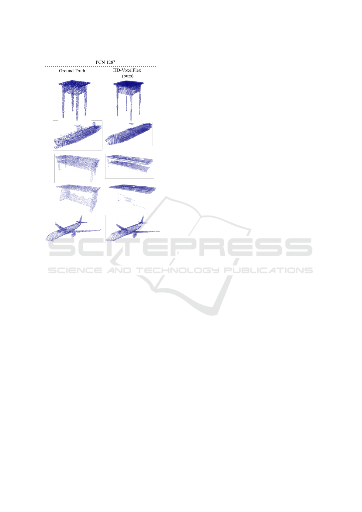
Figure 13: The qualitative renderings of 128

voxel grid

given PCN dataset. The PCN dataset contains a sparser

representation of the models (16384 points per model, 8

classes); thus, on average, only 0.7% of ﬁlled voxel cells

are engaged. Nonetheless, HD-VoxelFlex demonstrates im-

pressive results, as seen from the visual samples, where HD-

VoxelFlex works well in the areas where the model is struc-

turally balanced and densely represented.

HD-VoxelFlex: Flexible High-Deﬁnition Voxel Grid Representation

219