Relationship Between Semantic Segmentation Model and Additional
Features for 3D Point Clouds Obtained from on-Vehicle LIDAR
Hisato Hashimoto and Shuichi Enokida
Graduate School of Computer Science and Systems Engineering, Kyushu Institute of Technology,
680-4 Kawazu, Iizuka-shi, Fukuoka, 820-8502, Japan
Keywords:
Semantic Segmentation, Point Cloud, Deep Learning.
Abstract:
The study delves into semantic segmentation’s role in recognizing regions within data, with a focus on im-
ages and 3D point clouds. While images from wide-angle cameras are prevalent, they falter in challenging
environments like low light. In such cases, LIDAR (Laser Imaging Detection and Ranging), despite its lower
resolution, excels. The combination of LIDAR and semantic segmentation proves effective for outdoor en-
vironment understanding. However, highly accurate models often demand substantial parameters, leading to
computational challenges. Techniques like knowledge distillation and pruning offer solutions, though with
possible accuracy trade-offs. This research introduces a strategy to merge feature descriptors, such as re-
flectance intensity and histograms, into the semantic segmentation model. This process balances accuracy
and computational efficiency. The findings suggest that incorporating feature descriptors suits smaller models,
while larger models can benefit from optimizing computation and utilizing feature descriptors for recognition
tasks. Ultimately, this research contributes to the evolution of resource-efficient semantic segmentation mod-
els for autonomous driving and similar fields.
1 INTRODUCTION
In recent years, recognition technology for the oper-
ating environment of autonomous transportation de-
vices, such as self-driving vehicles, has been gaining
attention worldwide. Various technical approaches
are continuously developed, and among them, seman-
tic segmentation is one effective method. Semantic
segmentation enables region recognition by assigning
attributes to individual elements of data, and it has
gained significant attention, particularly with the ad-
vancement of deep learning models. Data used for se-
mantic segmentation processing include images and
3D point clouds. Generally, wide-angle cameras are
used for capturing images in vehicles, while LIDAR
is employed for obtaining 3D point clouds in broad
scenes like traffic environments. Cameras have high
resolutions and are commonly used sensors not only
in the field of autonomous driving but also in a wide
range of applications such as robotics and household
appliances. However, cameras can become unstable
in environments with wide dynamic ranges, like ur-
ban areas at night. On the other hand, while LI-
DAR has the disadvantage of lower resolution com-
pared to cameras, it can measure without being af-
?
good
good
?
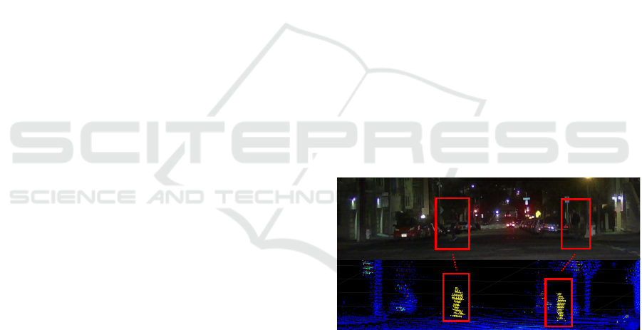
Figure 1: Robust measurement performance of LIDAR in
low-light environments. While identification is challenging
with camera (above), LIDAR (below) accurately captures
the human form(Created from (Xiao et al., 2021)’s data).
fected by low-light conditions or external light inter-
ference. As shown in Figure 1, in captured camera
images, dark areas can result in unclear distinctions,
making discrimination difficult in low-light environ-
ments. In contrast, LIDAR-derived point clouds can
capture the point clouds of multiple individuals even
in such low-illumination scenarios. This is because
LIDAR is an active sensor while the camera is a pas-
sive sensor. Efforts towards achieving autonomous
platooning without the need for special road infras-
tructure(Toshiki Isogai, 2016) also emphasize the ad-
Hashimoto, H. and Enokida, S.
Relationship Between Semantic Segmentation Model and Additional Features for 3D Point Clouds Obtained from on-Vehicle LIDAR.
DOI: 10.5220/0012374400003660
Paper published under CC license (CC BY-NC-ND 4.0)
In Proceedings of the 19th International Joint Conference on Computer Vision, Imaging and Computer Graphics Theory and Applications (VISIGRAPP 2024) - Volume 2: VISAPP, pages
547-553
ISBN: 978-989-758-679-8; ISSN: 2184-4321
Proceedings Copyright © 2024 by SCITEPRESS – Science and Technology Publications, Lda.
547

vantages of the active approach, and LIDAR is being
adopted for this purpose. This combination of the ro-
bustness to illumination changes offered by LIDAR
and the ability to comprehend multiple classes of re-
gions at once through semantic segmentation proves
to be an effective approach for outdoor environment
recognition. Therefore, in this study, we focus on LI-
DAR and target semantic segmentation for 3D point
clouds acquired by LIDAR.
2 RELATED WORKS
2.1 Image Semantic Segmentation
Semantic segmentation plays a crucial role in tasks
involving region recognition within data. While tra-
ditional image classification mainly involved abstrac-
tion of numerous pixels into higher-dimensional rep-
resentations, semantic segmentation requires the out-
put of information for each pixel, demanding the
restoration of the abstracted information back to
the original resolution. Early semantic segmenta-
tion methods(Shi and Malik, 2000; Felzenszwalb and
Huttenlocher, 2004) represented images as graphs
and utilized graph-cut algorithms to perform seg-
mentation based on the relationships between neigh-
boring pixels. Subsequently, with the rapid devel-
opment of deep learning, the Fully Convolutional
Network (FCN)(Long et al., 2015) was introduced,
which marked the beginning of semantic segmen-
tation methods using neural network architectures.
FCNs, primarily used for semantic segmentation,
forgo fully connected layers and instead rely on typi-
cal convolutional and pooling layers, thereby preserv-
ing position information across the entire input im-
age and enabling image segmentation. Furthermore,
the U-Net(Ronneberger et al., 2015) architecture in-
troduced an encoder-decoder pair, enabling finer seg-
mentation by aggregating information spatially and
then expanding it back to the original space. The
DeepLab series(Chen et al., 2017; Chen et al., 2018)
further improved segmentation accuracy by combin-
ing atrous convolution and fully connected condi-
tional random fields (CRF).
2.2 Point Cloud Semantic Segmentation
The evolution of research on 2D images gradually be-
gan to influence the field of semantic segmentation
for 3D point clouds. VoxNet(Maturana and Scherer,
2015) was the first model to convert 3D point clouds
into cuboids called voxel grids and apply 3D CNNs.
However, voxelization can be computationally expen-
sive and fail to fully account for the disorder and
sparsity of 3D data. PointNet(Qi et al., 2017) be-
came the first deep learning model that directly pro-
cessed individual points independently, thus address-
ing the disorder and sparsity of point clouds. More
recently, SqueezeSeg(Wu et al., 2018) was proposed,
enabling deep learning-based semantic segmentation
on LIDAR-derived point cloud data. SqueezeSeg
leverages the advantages of aligned point cloud data
by utilizing a combination of feature extraction from
image-based CNNs and class classification through
fully connected layers. This approach achieves effi-
cient and accurate segmentation. The advancement
of deep learning significantly improved accuracy, but
models designed for high accuracy often come with
a substantial number of parameters, demanding high
computational power. Particularly in the realm of se-
mantic classification models, increasing the number
of channels or layers in deep learning models is a
straightforward way to improve accuracy, but for de-
ployment on edge devices, aiming for high accuracy
while keeping the model small becomes crucial.
3 RELATIONSHIP BETWEEN
MODEL SIZE AND ACCURACY
Semantic classification models for point clouds in-
clude SqueezeSeg, which employs the image classi-
fication CNN SqueezeNet(Iandola et al., 2016), and
PointNet, which processes each point through the
same Multi Layer Perceptron (MLP) and addresses
the invariance of point order through max-pooling.
Both are capable of achieving semantic classification
for 3D point clouds, but CNNs exhibit better per-
formance compared to MLPs, thanks to their abil-
ity to exploit local correlations (as demonstrated by
AlexNet(Krizhevsky et al., 2012)). Moreover, CNNs
are more efficient and lightweight due to fewer pa-
rameters than MLPs, which is why CNN-based mod-
els have become mainstream in recognition tasks
since the introduction of AlexNet. In general, the ac-
curacy of CNNs tends to increase with more channels
in each layer, but this comes at the cost of increased
computation and processing time. When models
become large, it’s common to compress them for
deployment on edge devices, achieving lightweight
and faster processing. Techniques frequently used
for model compression include ”knowledge distilla-
tion(Hinton et al., 2015)”, ”quantization(Wu et al.,
2020)” and ”network pruning(Han et al., 2015)” as
discussed by Anthony Berthelier et al.(Anthony et al.,
2021). Knowledge distillation involves training a stu-
dent model to minimize the loss between the output
VISAPP 2024 - 19th International Conference on Computer Vision Theory and Applications
548
of the pre-compression teacher model and the post-
compression student model, transferring knowledge
from the teacher to the student. Quantization reduces
the memory usage of model parameters (weights, etc.)
by representing them with fewer bits, while keeping
the network structure unchanged. Network pruning
involves removing nodes with small weights, achiev-
ing model compression while maintaining accuracy.
However, these methods can lead to significant ac-
curacy degradation depending on the compression
goals. Therefore, in this study, we investigate the
relationship between various features and model ar-
chitecture with the goal of lightweighting the model
while maintaining comparable accuracy to the origi-
nal model. This is achieved by combining a reduced
architecture obtained by pruning nodes before train-
ing with a method for improving accuracy through
feature addition.
4 FEATURES EXTRACTED
FROM POINT CLOUDS
ACQUIRED FROM
ON-VEHICLE LIDAR
For the additional features to the model’s input in this
study, ”reflectance intensity”, ”reflectance intensity
histogram” representing the distribution of reflectance
intensities in neighboring point clouds, and ”Fast
Point Feature Histograms (FPFH)(Rusu et al., 2009)”
describing surface shapes through histogramizing the
distribution of normals based on the normals of the
points of interest and their neighbors are used. While
3D coordinates and reflectance intensities, directly
obtained from LIDAR, are used as input features, this
study investigates the impact of reflectance intensity
histograms and FPFH, which describe features out-
side the model, through comparative experiments to
assess their effectiveness.
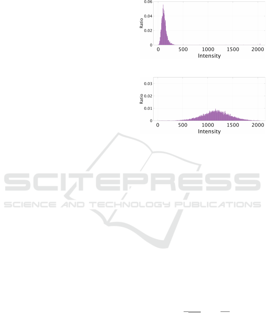
4.1 Reflectance Intensity
Reflectance intensity is a type of measurement data
obtained from LIDAR, calculated from the attenua-
tion rate of the laser light emitted from the LIDAR’s
light emitter, reflected from the target object, and re-
ceived by the LIDAR’s light receiver. As shown in
Figure 2, the reflectance intensity for artificial sur-
faces mainly composed of black asphalt has a mode
value of 106, indicating a narrow distribution. On the
other hand, as shown in Figure 3, the reflectance in-
tensity for natural surfaces mainly composed of green
grass has a mode value of 1156, stronger than asphalt,
Figure 2: Distribution of reflectance intensity(Asphalt:
black artificial object).
Figure 3: Distribution of reflectance intensity(Grass: green
natural object).
with a wider distribution. Therefore, reflectance in-
tensity serves as a feature that can reflect differences
in color and between artificial and natural objects.
4.2 Reflectance Intensity Histogram
The reflection intensity histogram is a novel feature
defined in this study, which involves histogramiz-
ing the occurrence distribution of reflection inten-
sities within the neighborhood points of an interest
point using weighted summation (as depicted in Fig-
ure 4). When directly summing the occurrence dis-
tribution within the neighborhood points, the correla-
tion with the interest point tends to weaken, causing
excessive blurring of information. Therefore, in this
study, the histogramization is performed while vary-
ing the weights based on the distance d
i
from the in-
terest point, thereby maintaining the correlation with
the interest point. The weight w
i
for the i-th point p
i
within the neighborhood points is defined using Equa-
tion (1), where σ is defined by Equation (2).
w
i
=
1
√
2πσ
2
exp
−
d
i
2
2σ
2
(1)
σ = ar (2)
(a : Attenuation Rate, r : Range of Point Search)
This feature’s dimensionality corresponds to the num-
ber of bins used for partitioning. In this paper, the
number of bins was set to 31, with values a and r set
to 1.8 and 0.5, respectively.
Relationship Between Semantic Segmentation Model and Additional Features for 3D Point Clouds Obtained from on-Vehicle LIDAR
549
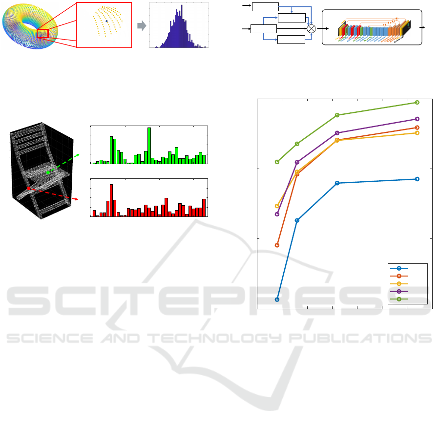
Figure 4: Creating a histogram of reflection intensity, af-
ter selecting points within a specified radius from the focal
point and creating a local point cloud, the reflectance in-
tensity of points contained in this local point cloud is the
subject of the histogram.
-400
-300
200
-200
-100
100
0
200
0
100
200
-100
0
300
Selected Indices on Point Cloud
-200
400
-200
FPFH Descriptors of Selected Indices
0 10 20 30
0
20
40
60
80
0 10 20 30
0
20
40
60
80
Figure 5: Feature Representation of FPFH. Green point on
the monotonous seat of the chair, red point on the complex
legs of the chair.
4.3 Fast Point Feature
Histograms(FPFH)
Fast Point Feature Histograms (FPFH) is a type of lo-
cal feature descriptor computed from 3D point cloud
data, aiming to achieve effective feature representa-
tion (33 dimensions) while maintaining compactness.
FPFH describes the surface shape by histogramiz-
ing the distribution relationship of normals between
an interest point and its neighboring points based on
their normals. The foundation of FPFH, Point Feature
Histograms (PFH)(Rusu et al., 2008b)(Rusu et al.,
2008a), captures geometric features around keypoints
by analyzing the normals’ directions of the keypoints’
vicinity. PFH creates pairs among all neighboring
points to build histograms, ensuring accurate results,
but it suffers from a significant computational cost. In
a point cloud with n points, the computational com-
plexity of PFH for a neighborhood size k is O(nK
2
).
To mitigate this computational burden, FPFH uses
only the links between keypoints and their neighbor-
ing points. By reducing these links, FPFH reduces
the computational complexity to O(nK). Figure 5 il-
lustrates an example of computed FPFH. Differences
in histograms can be observed between the seat (red
points) and legs (green points) of the chair.
Focal Loss
Fig. 2. Network structure of the proposed SqueezeSegV2 model for road-object segmentation from 3D LiDAR point clouds.
Input tensor
MaxPooling
77, C
Conv 11 &
Relu, C/16
Conv 11 &
Sigmoid, C
Element-wise
Multiply
Output tensor
H
W
C
H
W
C
Fig. 3. Structure of Context Aggregation Module.
a simple numerical experiment, where we randomly sample
an input tensor and feed it into a 3 ⇥3 convolution filter. We
randomly drop out some pixels from the input tensor, and as
shown in Fig. 4, as we increase the dropout probability, the
difference between the errors of the corrupted output and the
original output also increases.
This problem not only impacts SqueezeSeg when trained
on real data, but also leads to a serious domain gap between
synthetic data and real data, since simulating realistic dropout
noise from the same distribution is very difficult.
To solve this problem, we propose a novel Context
Aggregation Module (CAM) to reduce the sensitivity to
dropout noise. As shown in Fig. 3, CAM starts with a max
pooling with a relatively large kernel size. The max pooling
aggregates contextual information around a pixel with a
much larger receptive field, and it is less sensitive to missing
data within its receptive field. Also, max pooling can be
computed efficiently even with a large kernel size. The max
pooling layer is then followed by two cascaded convolution
layers with a ReLU activation in between. Following [32],
we use the sigmoid function to normalize the output of the
module and use an element-wise multiplication to combine
the output with the input. As shown in Fig. 4, the proposed
module is much less sensitive to dropout noise – with the
same corrupted input data, the error is significantly reduced.
In SqueezeSegV2, we insert CAM after the output of the
first three modules (1 convolution layer and 2 FireModules),
where the receptive fields of the filters are small. As can
be seen in later experiments, CAM 1) significantly improves
the accuracy when trained on real data, and 2) significantly
reduces the domain gap while trained on synthetic data and
testing on real data.
B. Focal Loss
LiDAR point clouds have a very imbalanced distribution
of point categories – there are many more background points
than there are foreground objects such as cars, pedestrians,
etc. This imbalanced distribution makes the model focus
more on easy-to-classify background points which contribute
0.0 0.1 0.2 0.3 0.4 0.5 0.6
0.0
0.2
0.4
0.6
0.8
1.0
Normalized error caused
by dropout noise
Dropout probability
w CAM
w/o CAM
Fig. 4. We feed a random tensor to a convolutional filter, one with CAM
before a 3 ⇥ 3 convolution filter and the other one without CAM. We
randomly add dropout noise to the input, and measure the output errors. As
we increase the dropout probability, the error also increases. For all dropout
probabilities, adding CAM improve the robustness towards the dropout noise
and therefore, the error is always smaller.
no useful learning signals, with the foreground objects not
being adequately addressed during training.
To address this problem, we replace the original cross
entropy loss from SqueezeSeg [2] with a focal loss [4].
The focal loss modulates the loss contribution from different
pixels and focuses on hard examples. For a given pixel label
t, and the predicted probability of p
t
, focal loss [4] adds a
modulating factor (1 p
t
)
to the cross entropy loss. The
focal loss for that pixel is thus
FL(p
t
)=(1 p
t
)
log (p
t
) (1)
When a pixel is mis-classified and p
t
is small, the modulating
factor is near 1 and the loss is unaffected. As p
t
! 1, the fac-
tor goes to 0, and the loss for well-classified pixels is down-
weighted. The focusing parameter smoothly adjusts the rate
at which well-classified examples are down-weighted. When
=0, the Focal Loss is equivalent to the Cross Entropy
Loss. As increases, the effect of the modulating factor is
likewise increased. We choose to be 2 in our experiments.
C. Other Improvements
LiDAR Mask: Besides the original (x, y, z, intensity,
depth) channels, we add one more channel – a binary mask
indicating if each pixel is missing or existing. As we can see
from Table I, the addition of the mask channel significantly
improves segmentation accuracy for cyclists.
Batch Normalization: Unlike SqueezeSeg [2], we also
add batch normalization (BN) [5] after every convolution
layer. The BN layer is designed to alleviate the issue of
internal covariate shift – a common problem for training
Figure 6: Input structure of features. Before inputting into
SqueezeSegV2, combine intensity, intensity histogram and
FPFH with 3D coordinates(xyz).
0 20 40 60 80 100 120 140
Model Size
0.75
0.8
0.85
0.9
Global Accuracy
Transition in Accuracy
xyz
xyzi
xyzf
xyzih
all
Figure 7: Accuracy transitions with changes in model
size(Plotting at four different model size : 16, 32, 64, 128),
blue: xyz only, red: with intensity, yellow: with FPFH, pur-
ple: intensity histogram, green: with all features.
5 EXPERIMENTS AND
DISCUSSIONS COMPARING
THE EFFECTIVENESS OF
VARIOUS FEATURES
In this study, a comparative experiment is conducted
using PandaSet(Xiao et al., 2021), which consists of
3D point cloud data collected from onboard LIDAR
sensors. The SqueezeSegV2 (Wu et al., 2019) archi-
tecture is employed to assess the effectiveness of var-
ious features. The experiment is structured as shown
in Figure 6. SqueezeSegV2 employs multiple lay-
ers of encoder modules to aggregate features, and the
base channel numbers (16, 32, 64, 128) that consti-
tute each layer are considered as the model sizes. The
number of layers is kept fixed. Five input patterns
are investigated: [xyz: 3D coordinates only, xyzi:
with added intensity, xyzih: with added intensity his-
VISAPP 2024 - 19th International Conference on Computer Vision Theory and Applications
550
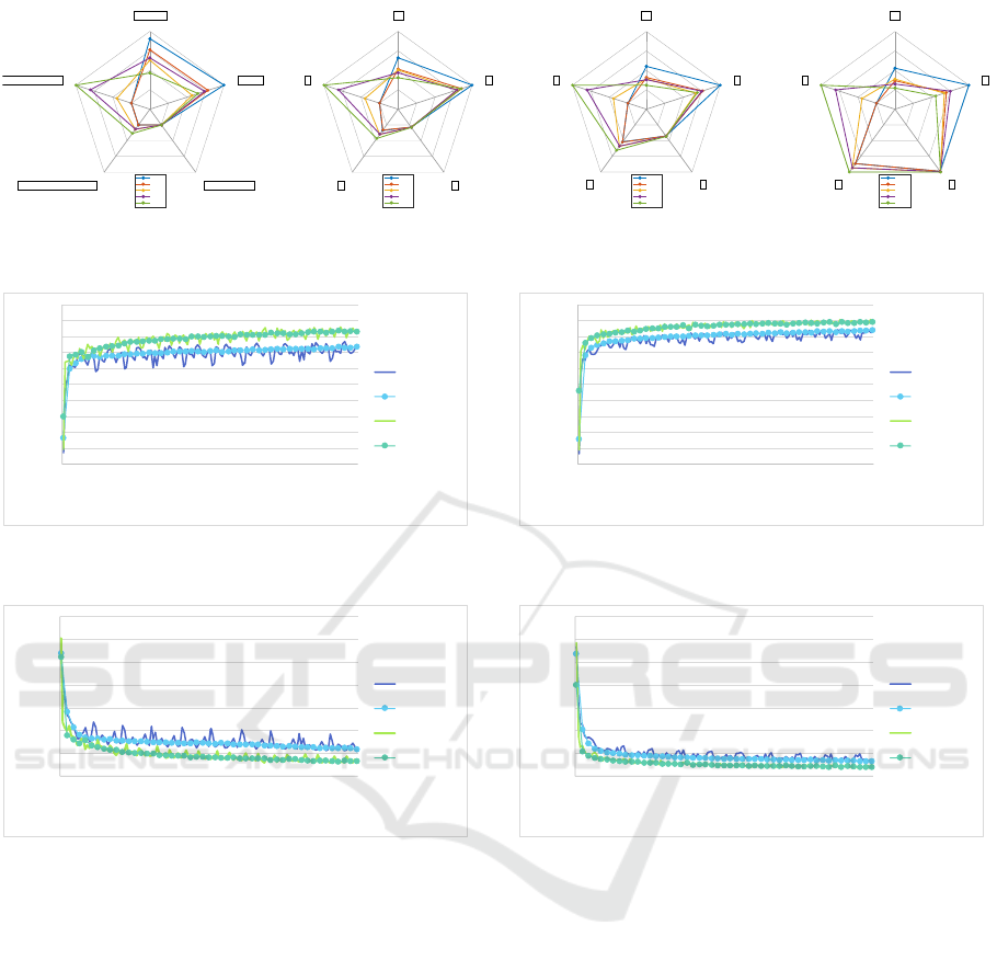
Radar chart based on each evaluation indicator : ChannelNum16
0.1
0.1
0.2
0.2
96.0
97.3
98.7
100.0
87848.0
1828796.3
3569744.7
5310693.0
1084.0
2264.0
3444.0
4624.0
0.0
4628.7
9257.3
13886.0
inA:inaccuracy
S:Similarity
P:Trainable ParametersM:GPU Memory Usage at Prediction
T:Feature Computation Cost
xyz
xyzi
xyzf
xyzih
all
Radar chart based on each evaluation indicator : ChannelNum32
0.1
0.1
0.2
0.2
96.0
97.3
98.7
100.0
87848.0
1828796.3
3569744.7
5310693.0
1084.0
2264.0
3444.0
4624.0
0.0
4628.7
9257.3
13886.0
inA
S
PM
T
xyz
xyzi
xyzf
xyzih
all
Radar chart based on each evaluation indicator : ChannelNum64
0.1
0.1
0.2
0.2
96.0
97.3
98.7
100.0
87848.0
1828796.3
3569744.7
5310693.0
1084.0
2264.0
3444.0
4624.0
0.0
4628.7
9257.3
13886.0
inA
S
PM
T
xyz
xyzi
xyzf
xyzih
all
Radar chart based on each evaluation indicator : ChannelNum128
0.1
0.1
0.2
0.2
96.0
97.3
98.7
100.0
87848.0
1828796.3
3569744.7
5310693.0
1084.0
2264.0
3444.0
4624.0
0.0
4628.7
9257.3
13886.0
inA
S
PM
T
xyz
xyzi
xyzf
xyzih
all
Figure 8: Radar chart based on each evaluation indicator(Model size from left to right: 16, 32, 64, 128), blue: xyz only, red:
with intensity, yellow: with FPFH, purple: intensity histogram, green: with all features.
0
10
20
30
40
50
60
70
80
90
100
1
100
200
300
400
500
600
700
800
900
1000
1100
1200
1300
1400
1500
1600
1700
1800
1900
2000
2100
2200
2300
2400
Accuracy[%]
iteration
train_16
val_16
train_128
val_128
Figure 9: [xyz-Only] Accuracy Transition During Training
for Maximum(128) and Minimum(16) Model Sizes.
0
0.1
0.2
0.3
0.4
0.5
0.6
0.7
1
100
200
300
400
500
600
700
800
900
1000
1100
1200
1300
1400
1500
1600
1700
1800
1900
2000
2100
2200
2300
2400
Loss
iteration
train_16
val_16
train_128
val_128
Figure 10: [xyz-Only] Loss Transition During Training for
Maximum(128) and Minimum(16) Model Sizes.
togram, xyzf: with added FPFH, all: with all features
added]. These input patterns are evaluated using four
model size variations (a total of 20 patterns) in the
range of model size variations mentioned above. The
evaluation is performed through three rounds of train-
ing and testing, and the results are averaged for anal-
ysis.
Figure 7 shows the transition in accuracy as the
model size is changed. From Figure 7, it is evident
that with model sizes of 32 for ’xyzi’, ’xyzih’, and
’xyzf’, and 16 for all, an accuracy of 0.8441 or higher
is achieved, comparable to the model size of 128 for
xyz. Additionally, it was confirmed that the conver-
gence of accuracy and loss becomes faster by adding
features, as observed in the transition results of accu-
racy shown in Figure 9 and Figure 11, and the tran-
sition results of loss shown in Figure 10 and Figure
12 during training. Moreover, the increase in GPU
0
10
20
30
40
50
60
70
80
90
100
1
100
200
300
400
500
600
700
800
900
1000
1100
1200
1300
1400
1500
1600
1700
1800
1900
2000
2100
2200
2300
2400
Accuracy[%]
iteration
train_16
val_16
train_128
val_128
Figure 11: [all-Features] Accuracy Transition During Train-
ing for Maximum(128) and Minimum(16) Model Sizes.
0
0.1
0.2
0.3
0.4
0.5
0.6
0.7
1
100
200
300
400
500
600
700
800
900
1000
1100
1200
1300
1400
1500
1600
1700
1800
1900
2000
2100
2200
2300
2400
Loss
iteration
train_16
val_16
train_128
val_128
Figure 12: [all-Features] Loss Transition During Training
for Maximum(128) and Minimum(16) Model Sizes.
memory due to feature addition is minimal compared
to the increase observed during model size expansion.
Therefore, it can be concluded that feature addition is
an effective approach for devices with stringent GPU
memory constraints, such as edge computing environ-
ments.
Additionally, to assess the impact of various fea-
tures on the model, five metrics are utilized: ”Inac-
curacy: inA”, ”Similarity: S”, ”Trainable Parame-
ters: P”, ”GPU Memory Usage at Prediction: M”, and
”Feature Computation Cost: T”. These metrics are
used to create a radar chart for a comprehensive eval-
uation. In this study, similarity refers to quantifying
the influence of each feature by vectorizing class-wise
accuracy when using various features together. This
is achieved by calculating the cosine similarity among
the vectors. The relative values are calculated by com-
paring them to the results obtained with only 3D co-
Relationship Between Semantic Segmentation Model and Additional Features for 3D Point Clouds Obtained from on-Vehicle LIDAR
551

ordinates for the same model size. When adding the
additional feature F, the accuracies of all 13 classes
are treated as a vector C
C
Cl
l
la
a
as
s
ss
s
sA
A
Ac
c
cc
c
c
F
with dimensions
1×13. The cosine similarity S is calculated by finding
the average cosine similarity between the C
C
Cl
l
la
a
as
s
ss
s
sA
A
Ac
c
cc
c
c
F
vectors obtained for each feature addition. This co-
sine similarity serves as a measure of the impact of
each feature on the class accuracies. Smaller values
indicate that a feature has a different impact on class
accuracies compared to other features. Feature com-
putation cost is evaluated using a relative scale based
on the time it takes to calculate the feature. The com-
putation time strongly depends on the CPU perfor-
mance, so a relative scale is defined using the compu-
tational cost of calculating the Euclidean distance as 1
and the cost of calculating the non-needed intensity as
0. It can be observed that there is a change in similar-
ity depending on the size of the model. Furthermore,
with an increase in model size, there is an increase
in GPU memory usage and trainable parameter count.
However, the increase in these values due to the ad-
dition of features is marginal. While adding all fea-
tures yields positive impacts on inaccuracy, the com-
putational cost of feature computation becomes eco-
nomically impractical. On the other hand, while fea-
ture addition doesn’t significantly affect GPU mem-
ory usage during inference, it does involve compu-
tation costs. Therefore, selecting appropriate features
based on the available CPU and GPU resources is cru-
cial when embedding the model into edge comput-
ing devices. Consequently, adding feature-descriptive
features is advantageous for smaller models, while for
larger models, it’s more beneficial to leave the fea-
ture description to the model itself to minimize fea-
ture computation costs.
6 CONCLUSIONS
In this paper, we propose a method to incorporate
additional features into the input of a semantic clas-
sification model. While evaluating the effective-
ness of these additional features, we aim to achieve
both model lightweighting and accuracy preservation.
Moving forward, we will focus on observing changes
in learning efficiency through feature integration, and
strive to adapt the model to be more compact while
maintaining high accuracy. Additionally, we will ex-
plore comprehensive evaluation methods that encom-
pass various performance metrics.
REFERENCES
Anthony, B., Thierry, C., Stefan, D., Christophe, G., and
Christophe, B. (2021). Deep Model Compression and
Architecture Optimization for Embedded Systems: A
Survey. Journal of Signal Processing Systems, vol.93,
pp.863-878.
Chen, L.-C., Papandreou, G., Kokkinos, I., Murphy, K., and
Yuille, A. L. (2017). Deeplab: Semantic image seg-
mentation with deep convolutional nets, atrous con-
volution, and fully connected crfs. IEEE transactions
on pattern analysis and machine intelligence, vol.40,
no.4, pp.834-848.
Chen, L.-C., Zhu, Y., Papandreou, G., Schroff, F., and
Adam, H. (2018). Encoder-decoder with atrous sep-
arable convolution for semantic image segmentation.
Proceedings of the European conference on computer
vision (ECCV), pp.801-818.
Felzenszwalb, P. F. and Huttenlocher, D. P. (2004). Effi-
cient graph-based image segmentation. International
journal of computer vision, vol.59, pp.167-181.
Han, S., Mao, H., and Dally, W. J. (2015). Deep compres-
sion: Compressing deep neural networks with prun-
ing, trained quantization and huffman coding. arXiv
preprint arXiv:1510.00149.
Hinton, G., Vinyals, O., and Dean, J. (2015). Distilling
the knowledge in a neural network. arXiv preprint
arXiv:1503.02531.
Iandola, F. N., Han, S., Moskewicz, M. W., Ashraf, K.,
Dally, W. J., and Keutzer, K. (2016). SqueezeNet:
AlexNet-level accuracy with 50x fewer parame-
ters and¡ 0.5 MB model size. arXiv preprint
arXiv:1602.07360.
Krizhevsky, A., Sutskever, I., and Hinton, G. E. (2012). Im-
agenet classification with deep convolutional neural
networks. Advances in neural information processing
systems, vol.25.
Long, J., Shelhamer, E., and Darrell, T. (2015). Fully con-
volutional networks for semantic segmentation. Pro-
ceedings of the IEEE conference on computer vision
and pattern recognition, pp.3431-3440.
Maturana, D. and Scherer, S. (2015). Voxnet: A 3d con-
volutional neural network for real-time object recog-
nition. 2015 IEEE/RSJ international conference on
intelligent robots and systems (IROS), pp.922-928.
Qi, C. R., Su, H., Mo, K., and Guibas, L. J. (2017). Pointnet:
Deep learning on point sets for 3d classification and
segmentation. Proceedings of the IEEE conference on
computer vision and pattern recognition, pp.652-660.
Ronneberger, O., Fischer, P., and Brox, T. (2015). U-net:
Convolutional networks for biomedical image seg-
mentation. Medical Image Computing and Computer-
Assisted Intervention–MICCAI 2015: 18th Interna-
tional Conference, Munich, Germany, October 5-9,
2015, Proceedings, Part III 18, pp.234-241.
Rusu, R. B., Blodow, N., and Beetz, M. (2009). Fast
point feature histograms (FPFH) for 3D registration.
2009 IEEE international conference on robotics and
automation, pp.3122-3217.
VISAPP 2024 - 19th International Conference on Computer Vision Theory and Applications
552

Rusu, R. B., Blodow, N., Marton, Z. C., and Beetz, M.
(2008a). Aligning point cloud views using persistent
feature histograms. 2008 IEEE/RSJ international con-
ference on intelligent robots and systems, pp.3384-
3391.
Rusu, R. B., Marton, Z. C., Blodow, N., and Beetz, M.
(2008b). Learning informative point classes for the
acquisition of object model maps. 2008 10th Interna-
tional Conference on Control, Automation, Robotics
and Vision, pp.643-650.
Shi, J. and Malik, J. (2000). Normalized cuts and image
segmentation. IEEE Transactions on pattern analysis
and machine intelligence, Vol.22 no.8, pp.888-905.
Toshiki Isogai, Mitsuyasu Matsuura, T. K. (2016). Emviron-
ment Recognition Technology for Trucks platooning.
DENSO TECHINICAL REVIEW, vol.21, pp.71-76.
Wu, B., Wan, A., Yue, X., and Keutzer, K. (2018). Squeeze-
seg: Convolutional neural nets with recurrent crf
for real-time road-object segmentation from 3d lidar
point cloud. 2018 IEEE international conference on
robotics and automation (ICRA), pp.1887-1893.
Wu, B., Zhou, X., Zhao, S., Yue, X., and Keutzer, K.
(2019). Squeezesegv2: Improved model structure and
unsupervised domain adaptation for road-object seg-
mentation from a lidar point cloud. 2019 interna-
tional conference on robotics and automation (ICRA),
pp.4376-4382.
Wu, H., Judd, P., Zhang, X., Isaev, M., and Micikevicius,
P. (2020). Integer quantization for deep learning in-
ference: Principles and empirical evaluation. arXiv
preprint arXiv:2004.09602.
Xiao, P., Shao, Z., Hao, S., Zhang, Z., Chai, X., Jiao, J.,
Li, Z., Wu, J., Sun, K., Jiang, K., et al. (2021). Pan-
daset: Advanced sensor suite dataset for autonomous
driving. 2021 IEEE International Intelligent Trans-
portation Systems Conference (ITSC), pp.3095-3101.
Relationship Between Semantic Segmentation Model and Additional Features for 3D Point Clouds Obtained from on-Vehicle LIDAR
553
