Neural Architecture Search for Bearing Fault Classiﬁcation

Edicson Santiago Bonilla Diaz

1,2 a

, Enrique Naredo

3 b

, Nicolas Francisco Mateo D

ıaz

3 c

Douglas Mota Dias

4 d

, Maria Alejandra Bonilla Diaz

2,5 e

, Susan Harnett

5 f

and Conor Ryan

4 g

Department of Electronic and Computer Engineering, University of Limerick, Limerick, Ireland

Eastway Reliability, Limerick, Ireland

Universidad del Caribe, Cancun, Mexico

Department of Computer Science and Information Systems, University of Limerick, Limerick, Ireland

School of Engineering, University of Limerick, Limerick, Ireland

Keywords:

Bearing Fault Classiﬁcation, Vibration Analysis, Neural Architecture Search, Hyperparameter Optimization.

Abstract:

In this research, we address bearing fault classiﬁcation by evaluating three neural network models: 1D Con-

volutional Neural Network (1D-CNN), CNN-Visual Geometry Group (CNN-VGG), and Long Short-Term

Memory (LSTM). Utilizing vibration data, our approach incorporates data augmentation to address the limited

availability of fault class data. A signiﬁcant aspect of our methodology is the application of neural architec-

ture search (NAS), which automates the evolution of network architectures, including hyperparameter tuning,

signiﬁcantly enhancing model training. Our use of early stopping strategies effectively prevents overﬁtting,

ensuring robust model generalization. The results highlight the potential of integrating advanced machine

learning models with NAS in bearing fault classiﬁcation and suggest possibilities for further improvements,

particularly in model differentiation for speciﬁc fault classes.

1 INTRODUCTION

Rotating machinery, including electric motors, tur-

bine generators, and aero-engines, are essential equip-

ment of modern industry (Liu et al., 2018), and bear-

ings are critical to keep in motion all this equipment.

The worldwide annual production in round numbers

is 10 billion bearings worldwide, and the bearing re-

placement due to damage or failure from this total

production is estimated at 0.5% or more precisely in

50 million parts (SKF-Group., 2017).

A common technique for monitoring and evalu-

ating the condition of industrial rotating equipment

components, such as bearings, is through vibration

analysis according to the standard ISO 15242-1:2015

(ISO, 2015), which speciﬁes the measuring methods

https://orcid.org/0009-0009-0831-4999

https://orcid.org/0000-0001-9818-911X

https://orcid.org/0000-0003-4799-6434

https://orcid.org/0000-0002-1783-6352

https://orcid.org/0009-0003-4074-7870

https://orcid.org/0009-0009-3112-9978

https://orcid.org/0000-0002-7002-5815

for vibration of rotating rolling bearings under estab-

lished measuring conditions, together with calibration

of the related measuring systems. A comprehensive

survey about analysis techniques is out of the scope

of this work; for interested readers, it is recommended

to read (Romanssini et al., 2023) to extend the knowl-

edge about this topic.

On the other hand, Industry 4.0, in general, has

revolutionized the way industrial companies work, in-

tegrating new technologies and increasing at the same

time the amount of data from the bearing analysis.

Despite the volume of previous research, the devel-

opment of efﬁcient and accurate solutions for bearing

fault classiﬁcation remains an ongoing challenge.

This research study speciﬁcally aims to address

this critical gap by: (i) developing machine learning

models for bearing fault classiﬁcation, (ii) optimizing

the models using neural architecture search, and (iii)

evaluating the performance improvement achieved by

the optimized models. It is envisaged that the success-

ful execution of this study will not only advance the

capabilities of vibration analysts, who are currently

heavily reliant on their expertise, but also counter the

limitations of existing methods for fault diagnosis of

288

Diaz, E., Naredo, E., Díaz, N., Dias, D., Diaz, M., Harnett, S. and Ryan, C.

Neural Architecture Search for Bearing Fault Classiﬁcation.

DOI: 10.5220/0012373100003636

Paper published under CC license (CC BY-NC-ND 4.0)

In Proceedings of the 16th International Conference on Agents and Artiﬁcial Intelligence (ICAART 2024) - Volume 2, pages 288-300

ISBN: 978-989-758-680-4; ISSN: 2184-433X

rotating machinery (Peng et al., 2020).

In this work, we used the CWRU bearings dataset

(CWRU-Dataset., 2023) as a case study to perform

a bearing fault classiﬁcation. The raw data (1-

dimensional) required a preprocessing step to ensure,

on one hand, getting the right format using Markov

Transition Field Images (2-dimensional MTF images)

for the models selected, and on the other to tackle the

reduced amount of data available, splitting the data

ﬁrst and then applying a data augmentation process.

The machine learning model selected in this work

to develop a classiﬁer is a neural network. We have

chosen two types of convolutional neural network

(CNN), 1-dimensional CNN (1D-CNN) and the vi-

sual Geometry Group CNN (CNN-VGG), to compare

against a Recurrent Neural Network (RNN); Long

Short-Term Memory (LSTM) (Li et al., 2022). Fur-

thermore, we used a neural architecture search (NAS)

to evolve better and optimized neural network archi-

tectures.

The main contributions of this research are: (i)

Bearing fault classiﬁcation using convolutional neu-

ral networks, (ii) Optimizing the manually designed

CNNs through a neural architecture search, and (iii)

Comparative analysis of manual and automated de-

signed CNNs architectures.

In summary, the aim of this research study was to

advance the current state of vibration analysis tech-

niques through the introduction and optimization of

machine learning models for the automated diagnosis

of bearing faults in rotating machinery.

The successful completion of this research

demonstrates signiﬁcant improvements to the indus-

try’s diagnostic capabilities, addressing an ongoing

challenge and, thus, delivering a meaningful contri-

bution to the ﬁeld of industrial predictive maintenance

(PdM) and condition monitoring. This approach rep-

resents an option for the bearing vibration measure-

ment methods contained in ISO 15242-1:2015.

The remainder of this paper is organized as fol-

lows: Section 2, delves into the basic concepts of

Rotating Equipment and PdM, convolutional neural

networks and neural architecture search. Section 3,

transitions into the introduction of the CWRU bear-

ings dataset and its preprocessing. Section 4 is dedi-

cated to explaining the experimental setup. Section 5,

presents the experimental results, and ﬁnally, all the

highlights and ﬁndings are shown in Section 6.

2 BACKGROUND

2.1 Rotating Equipment

Rotating equipment is crucial in numerous industries

and essential for critical processes in sectors such

as manufacturing and energy production. Common

types include electrical motors, gearboxes, and cen-

trifugal pumps, all having similar components allow-

ing for rotation, with bearings being the most vital.

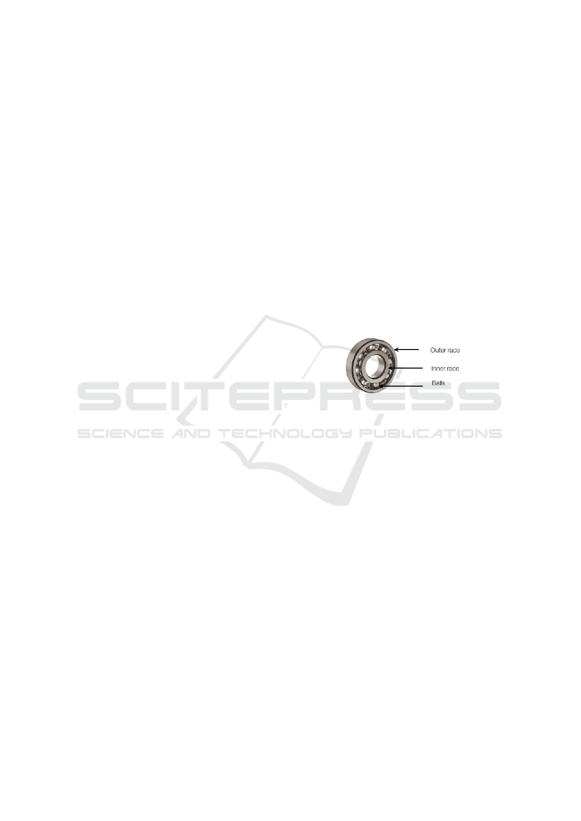
Bearings, consisting of an inner ring, outer ring,

cage, and rolling elements, allow rotation at different

speeds and support varied loads. Figure 1 shows the

key components of a ball bearing. Service life de-

pends on various factors, including load, size, lubri-

cation, and environmental conditions (SKF-Group.,

2023). While calculating bearing life is crucial during

design, it is not practical for maintenance decisions.

Utilizing condition-based monitoring of bearings has

demonstrated enhanced efﬁcacy over routine sched-

uled maintenance in ensuring equipment reliability.

Figure 1: Bearing parts (SKF-Group., 2017).

2.2 Predictive Maintenance

PdM measures efﬁciency, productivity, and the re-

maining life of equipment with regard to the schedul-

ing of repairs prior to breakdown occurrence. (Sakib

and Wuest, 2018). PdM uses condition monitoring

(CM) technologies to predict the condition of a sys-

tem, where vibration analysis (VA) is one of the most

versatile technologies used.

If CM detects an anomaly, then a diagnosis is

completed, and the necessary actions, such as bearing

lubrication, bearing replacement, etc., are scheduled

and conducted to ensure the system is maintained in

satisfactory condition.

VA is a technology that can be used for machine

condition diagnosis, and it can detect potential fail-

ures at an early stage. A typical process analysis in-

cludes evaluating the overall vibration value, raw sig-

nal (time domain), spectrum (frequency domain), and

machine history. In theory, an analysis can be con-

ducted using only raw signals, given that these signals

encapsulate the complete vibrational data of the unit.

Neural Architecture Search for Bearing Fault Classiﬁcation

289

2.3 Convolutional Neural Networks

1D-CNNs are a specialized type of neural network

primarily used for processing and analysing time-

series data (Goodfellow et al., 2016). This architec-

ture is well-suited to exploit local and temporal de-

pendencies by applying a series of convolutional ﬁl-

ters, enabling the detection of patterns across different

sections of the input data.

Among the available 1D-CNNs found in the liter-

ature, we began with a simple architecture inspired

by the one used by (Goodfellow et al., 2016). In

this study, a 1D-CNN can be highly effective as it is

designed to interpret the dependencies in time-series

data. It can recognize local patterns in the vibra-

tion data and temporal dynamics (Goodfellow et al.,

2016), making it an excellent tool for the task re-

quired. Authors in (Pinedo-Sanchez et al., 2020) pro-

posed a CNN model based on AlexNet architecture to

classify the wear level and diagnose the rotating bear-

ing system. Other CNN-based applications have been

used to make failure predictions in roller bearings; in

(Li et al., 2017), they combine CNN with the im-

proved Dempster-Shafer theory, while in (Xia et al.,

2017), the CNN performs fault diagnosis on rotat-

ing machines, incorporating sensor fusion to achieve

higher and more robust diagnostic accuracy.

2.4 CNN - Visual Geometric Group

CNN-VGG are a type of deep learning model initially

developed for image recognition tasks (Simonyan and

Zisserman, 2014). These networks are characterized

by simplicity, exclusively employing 3x3 convolu-

tional layers stacked atop one another in increasing

depth. The VGG architecture primarily consists of

convolutional layers, followed by pooling layers, and

then fully connected layers towards the output.

The convolutional layers detect spatial patterns in

the image data, followed by pooling layers that re-

duce the spatial dimensions while retaining the most

valuable information. The simplicity of VGG’s archi-

tecture makes it attractive for tasks requiring feature

extraction from images, including the 2D MTF im-

ages in this study.

2.5 Long Short-Term Memory

Long Short-Term Memory (LSTM) networks, intro-

duced by Hochreiter and Schmidhuber in 1997, are

a subtype of recurrent neural network (RNN) specif-

ically designed to overcome the limitations of tradi-

tional RNNs, especially when it comes to long-term

dependencies (Hochreiter and Schmidhuber, 1997).

LSTMs have demonstrated high effectiveness in

time-series data analysis due to their capacity to store

information over extended periods, making them par-

ticularly useful for the vibration data in this research

study. The typical architecture of a model comprises

an LSTM layer (whose size depends on the input

data), followed by various layers, such as dropout (to

prevent overﬁtting) and dense layers (serving as the

ﬁnal output layer).

2.6 Neural Architecture Search

Neural architecture design is typically performed

manually by human experts, following a time-

consuming trial-and-error process. In this work, we

used an automated approach named neural architec-

ture search (NAS). Even though there are several ap-

proaches to implementing NAS (Elsken et al., 2019),

in this work, we focus on using evolutionary algo-

rithms as the search engine. We selected a genetic

algorithm (GA) (Montana and Davis, 1989; Ahmed

et al., 2020; Laredo et al., 2019) to perform the ar-

chitecture search, and more speciﬁcally we follow the

ideas taken from (Houreh et al., 2021). The Hyper

Neural Architecture Search (HNAS) aims to design

the model’s architecture automatically using NAS to

explore the neural network architecture search space.

In this study, we take a similar approach as HNAS to

evolve 1-CNN, CNN-VGG type and LSTM architec-

tures, which is shown in Algorithm 1.

In HNAS, the individuals I represent solutions to

a problem which can be deﬁned by three elements:

β is the phenotype, G is the genotype, and S is the

score. The Genotype is a binary string, the phenotype

is the neural network architecture, and the score is de-

termined by the ﬁtness function. The genotype G en-

codes a set of relevant features of a neural network ar-

chitecture by a set of genes [g

, g

, ..., g

], each g

con-

sisting of an array of bits [b

, b

, ..., b

], where k is the

maximum number of bits used to encode the choices

of a given feature. The phenotype β decodes from G

different features depending on the model to be opti-

mized; for example, for a 1D-CNN the β is given by

learning rate (LR), number of ﬁlters (NF), ﬁlter size

(FS), pooling size (PS), and the number of dense units

(DU), or in another format β = [LR,NF,FS,PS,DU].

More details about β for each model architecture can

be found in section 4.2 Architecture Optimization.

3 DATASET

In this study, the CWRU bearings dataset was utilized.

The data represented the vibration time series of vari-

ICAART 2024 - 16th International Conference on Agents and Artiﬁcial Intelligence

290

Algorithm 1: HNAS.

Input: G = [g

, g

, ..., g

] // Representation

Output: best I

// Best architecture for a

given model

1 I

← (G, β, S) // S=score

2 β = [LR, NF, FS, PS, DU] S = ∅

// this example of β is for 1D-CNN

3 Q

t=0

← I

// Initial population

4 while t < m // m = max generations

5 do

6 Evaluate each phenotype β ∈ Q

t−1

7 S(I

) ← eval(β

) assign ﬁtness score

8 Select parents from Q

t−1

using S

9 Genetic operations on G

of selected parents

10 Q

← (G, β) offspring (new pop)

11 t ← t + 1

12 Return I

from Q

with the best S.

ous bearing faults and was collected using a vibration

sensor (accelerometer) mounted onto a testing motor.

Each class within this dataset was represented by a

single large ﬁle consisting of approximately 500,000

data points and was 1-dimensional (1D).

For this study, 10 classes were selected, compris-

ing a normal bearing class and three different fault

types, each with three severities. The fault severities

were categorized based on the diameter dimensions

of the damage within the bearing (0.007 inches, 0.014

inches, and 0.021 inches) and were separately intro-

duced at the inner raceway, rolling element (i.e., ball),

and outer raceway. Table 1 demonstrates the allocated

class distribution per bearing fault type for the model

training and testing.

Table 1: Bearing Fault Type and Class number assigned.

Fault Type Class

normal bearing 0

inner race 007 1

inner race 014 2

inner race 021 3

outer race 007 4

outer race 014 5

outer race 021 6

ball 007 7

ball 014 8

ball 021 9

3.1 Data Preprocessing

In machine learning tasks, particularly with limited

datasets, it is crucial to implement strategies that al-

low for robust model training and evaluation. One

such challenge encountered in this work was limited

data availability, which could have led to model over-

ﬁtting. Two strategies employed to mitigate this prob-

lem were data splitting and data augmentation. More-

over, to ensure the data adhered to the appropriate for-

mat for certain models, the 1-dimensional raw data

was transformed into 2-dimensional images. This was

achieved using the MTF.

3.2 Data Splitting and Data

Augmentation

Taking into consideration that the raw data from the

CWRU dataset comprised one large ﬁle per class,

with approximately 487,424 data points each, it was

essential to split each ﬁle into smaller blocks, which

were suitable for training machine learning models.

Each block was chosen to be of 2048 data points; this

number was set based on the experience of a vibration

analyst. In comparison, (Chuya-Sumba et al., 2022)

used blocks of 1004 data points.

Through the application of a normal spilt, the orig-

inal dataset of 487,424 data points would have cre-

ated 237 blocks. In order to increase the data volume,

a data augmentation technique was chosen, which

entailed an overlapping scheme during block split-

ting. This process generated slightly modiﬁed ver-

sions of existing data through the formation of over-

lapping data blocks with a deﬁned stride length. Thus,

each block shared some data points with its preceding

block while some new data points were introduced

(equal to the stride length). The resulting new size

of the data aligns with Equation 1 (Yan et al., 2022):

N =

L − l

+ 1, (1)

where N denotes the new size, L signiﬁes the original

size, l represents the block size, and s is the step or

stride.

The augmentation process applied for this study

correlated with the creation of each new block, shar-

ing 1948 data points with the previous block, with

the inclusion of 100 new data points. Figure 2 is a

representation of the block creation process with the

use of overlapping. The approach is similar to the

one used by (Yan et al., 2022). As a result, the aug-

mented dataset contained approximately 4036 blocks

per class or 9,904,128 data points. This data was used

directly to feed the 1D-CNN model.

3.3 Markov Transition Field

CNN and LSTM models require 2-dimensional in-

put data, as these models are mainly used for image

classiﬁcation and sequence prediction. Converting

Neural Architecture Search for Bearing Fault Classiﬁcation

291

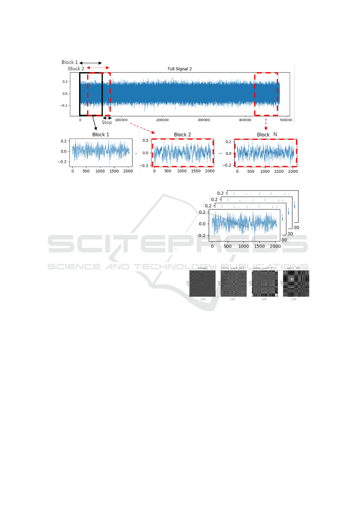
Figure 2: Representation of the block creation process with the use of splitting and overlapping.

raw 1-dimensional data into 2-dimensional is a sig-

niﬁcant task. The transformation needs to retain as

much detail as possible. Each time series block was

1-dimensional (2048,1) and required conversion into

2-dimensional to enable input for the CNN and LSTM

models. To achieve this, a Markov Transition Field

(MTF) class was used from the ‘pyts.image’ module

(Faouzi et al., 2017), a technique not previously re-

ported in similar research. This conversion resulted in

a 2-dimensional image that captured the spatial rela-

tionships between neighbouring values in the original

data. The ‘MTF’ class provides ﬂexibility in deter-

mining the resulting image’s dimensions. After mul-

tiple trials with varying sizes, 128x128 pixels (128,

128, 1) were selected, as this offered a suitable trade-

off between result quality and memory consumption.

Figure 3 displays 2048 data point sample blocks

in 1-dimensional format, while Figure 4 shows the

corresponding MTF image, obtained by transforming

these 1-dimensional blocks into a 2-dimensional for-

mat.

After augmenting and transforming the data, it

was divided into training and testing sets for all ex-

periments, adhering to the standard 80/20.

4 EXPERIMENTAL SETUP

The aim of this study was to develop machine learning

models to tackle the bearing fault classiﬁcation chal-

lenge. This was completed with six different exper-

iments; the ﬁrst three comprised a manual design of

1D-CNN, CNN-VGG type and LSTM architectures,

and the last three comprised automatic optimization

of previously named architectures via NAS. Addition-

Figure 3: Sample 1-dimensional raw data blocks with 2048

datapoints (2048, 1).

Figure 4: Sample MTF 2-dimensional images for different

classes (128, 128, 1).

ally, preprocessing the dataset was essential to en-

hance its robustness for training and ensure it was in

the appropriate format. A high-level representation of

the research methodology is shown in Figure 5.

4.1 Manual Design

Using the foundational work of (Chuya-Sumba et al.,

2022) and (Wang et al., 2022a) as a starting point, we

explored 1D-CNNs for processing one-dimensional

data such as vibration signals from bearings. These

algorithms proﬁciently identify temporal patterns,

making them optimal for bearing fault diagnosis.

(Chuya-Sumba et al., 2022) demonstrated promis-

ing results on two datasets with their deep learning

method. In contrast, (Wang et al., 2022a) proposed

ICAART 2024 - 16th International Conference on Agents and Artiﬁcial Intelligence

292

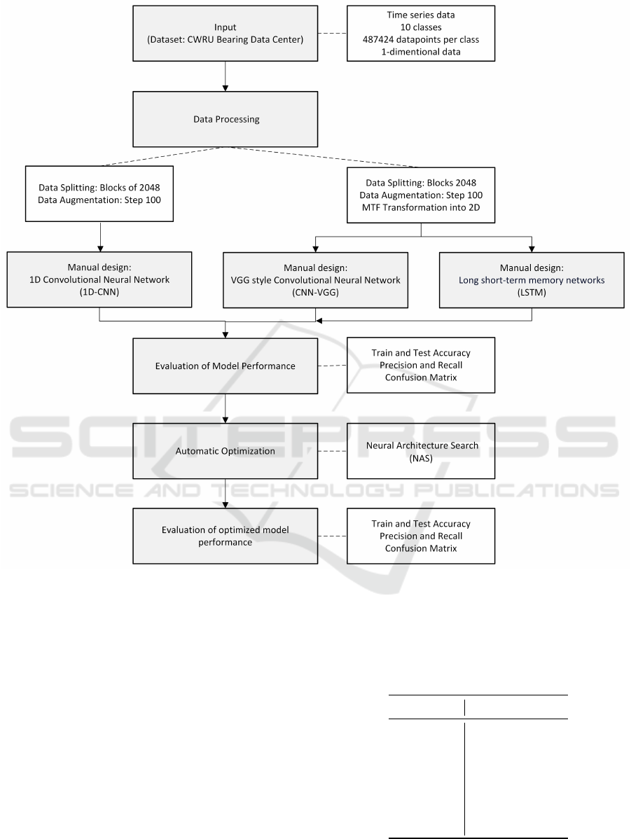
Figure 5: Research methodology ﬂowchart.

a simpler 1D-CNN architecture. Despite the signif-

icant contributions of both studies to bearing fault

diagnosis, neither delved into hyperparameter opti-

mization, suggesting an avenue for future research en-

hancements.

In this ﬁrst experiment, the parameters used to run

the 1D-CNN architecture were two convolutional 1D

layers, one MaxPooling1D layer, one dropout layer,

one ﬂatten layer, one dense layer with activation ‘relu’

and ﬁnally, one dense layer with softmax activation to

perform the classiﬁcation as outlined in Table 2. For

this architecture, the following hyperparameters were

chosen manually: learning rate, number of ﬁlters, ﬁl-

ter size (number of kernels), pooling size, and number

of dense units.

Similar to the ﬁrst experiment, the second experi-

ment was designed. The basic architecture of a CNN-

Table 2: 1D-CNN model summary, Conv1D: Conv1D

(None, 2048, 64), Conv1D: Conv1D (None, 2048, 64),

Max1D: MaxPooling1D (None, 1023, 64), Dropout:

Dropout (None, 1023, 64), Flatten: Flatten (None, 65472),

Dense100: Dense (None, 100), Dense10: Dense (None,

10).

CNN type Parameters

Conv1D Filter size = 3

Max1D Pool size = 2

Dropout Dropout = 0.5

Flatten Yes

Dense100 Activ.: relu

Dense10 Activ.: softmax

VGG type model requires multiple convolutional lay-

ers, each followed by a max-pooling layer (Scanlan,

Neural Architecture Search for Bearing Fault Classiﬁcation

293

2023). Dropout layers were also used to prevent over-

ﬁtting. After these layers, a ﬂattened layer was ap-

plied and connected to two dense layers. The last

layer used a softmax activation function to produce

a probability output for each of the 10 classes in the

bearing dataset, as outlined in Table 3. For this ar-

chitecture, these hyperparameters were manually cho-

sen: learning rate, number of ﬁlters on each convolu-

tional block, ﬁlter size, pooling size and the number

of dense units.

Table 3: CNN-VGG type model summary, Conv2D:

Conv2D (None, 128, 128, 32), Max2D: MaxPooling2D

(None, 64, 64, 32), Conv2D64: Conv2D (None, 64, 64,

64), Max2Db: MaxPooling2D (None, 32, 32, 64), Flat-

ten: Flatten (None, 65536), Dense128: Dense (None, 128),

Dropout: Dropout (None, 128), Dense10: Dense (None,

10).

CNN type Parameters

Conv2D Filter size = 3x3

Max2D Pool size = 2x2

Conv2D Filter size = 3x3

Conv2D64 Filter size = 3x3

Max2Db Pool size = 2x2

Flatten Yes

Dense128 Activ.: relu

Dropout Dropout = 0.5

Dense10 Activ.: softmax

In the last experiment, an LSTM model was em-

ployed. The choice in LSTM was guided by its ca-

pability to capture long-term dependencies in sequen-

tial data, which is beneﬁcial in the context of bearing

fault classiﬁcation (Liu et al., 2021). The model was

designed to consist of a single LSTM layer with 128

units and an output layer with ten units for the classi-

ﬁcation of ten classes, as shown in Table 4.

Table 4: LSTM model summary.

CNN type Parameters

LSTM (None, 128) Lstm units = 128

Dense (None, 10) Activ.: softmax

4.2 Architecture Optimization

We adopted a neural architecture search strategy sim-

ilar to HNAS, including the parameters delineated in

Table 5. To automate the optimization of architec-

tures, we meticulously reﬁned the hyperparameters

for the models in experiments one, two, and three, uti-

lizing the sets of parameters enumerated in Tables 6,

7, and 8, respectively. Figure 6 depicts the algorithm

employed to reﬁne the 1D-CNN model from exper-

iment one. For the subsequent experiments involv-

ing the CNN-VGG and LSTM models, the optimiza-

tion methodologies were analogous, with tailored ad-

justments in the genome to accommodate the unique

characteristics of each model.

Table 5: Main parameters used to run the NAS.

Parameter Value

Total generations 10

Population Size 5

Crossover Rate 0.5

Mutation Rate 0.2

Epochs 50

The genome was deﬁned for the NAS as the list of

hyperparameters to optimize changes on each model.

For the 1D-CNN, the genome was formed by learn-

ing rate (LR), number of ﬁlters (NF), ﬁlter size (FS),

pooling size (PS), and the number of dense units

(DU). Table 6 outlines the proposed number of genes

and the number of choices per gene for the 1D-CNN

model.

Table 6: Genome for the 1D-CNN model.

Parameter Choices

LR 0.0001, 0.001, 0.01, 0.1

NF 16, 32, 64, 128

FS 2, 3, 4, 5

PS 2, 3, 4

DU 32, 64, 96, 128

Similarly, for the CNN-VGG type model, the

genome was formed by the following hyperparame-

ters: learning rate (LR), number of ﬁlters in the ﬁrst

two convolutional layers (NF), number of ﬁlters in the

following two convolutional layers (NF2), ﬁlter size

(FS), pooling size (PS), and the number of dense units

(DU), see Table 7 .

Table 7: Genome for the CNN-VGG type model.

Parameter Choices

LR 0.0001, 0.001, 0.01, 0.1

NF 16, 32, 64, 128

NF2 16, 32, 64, 128

FS 2, 3, 4, 5

PS 2, 3, 4

DU 32, 64, 96, 128

For the LSTM model, the genome was formed by

the following hyperparameters: learning rate (LR),

number of LSTM units (LU), number of dense units

ICAART 2024 - 16th International Conference on Agents and Artiﬁcial Intelligence

294

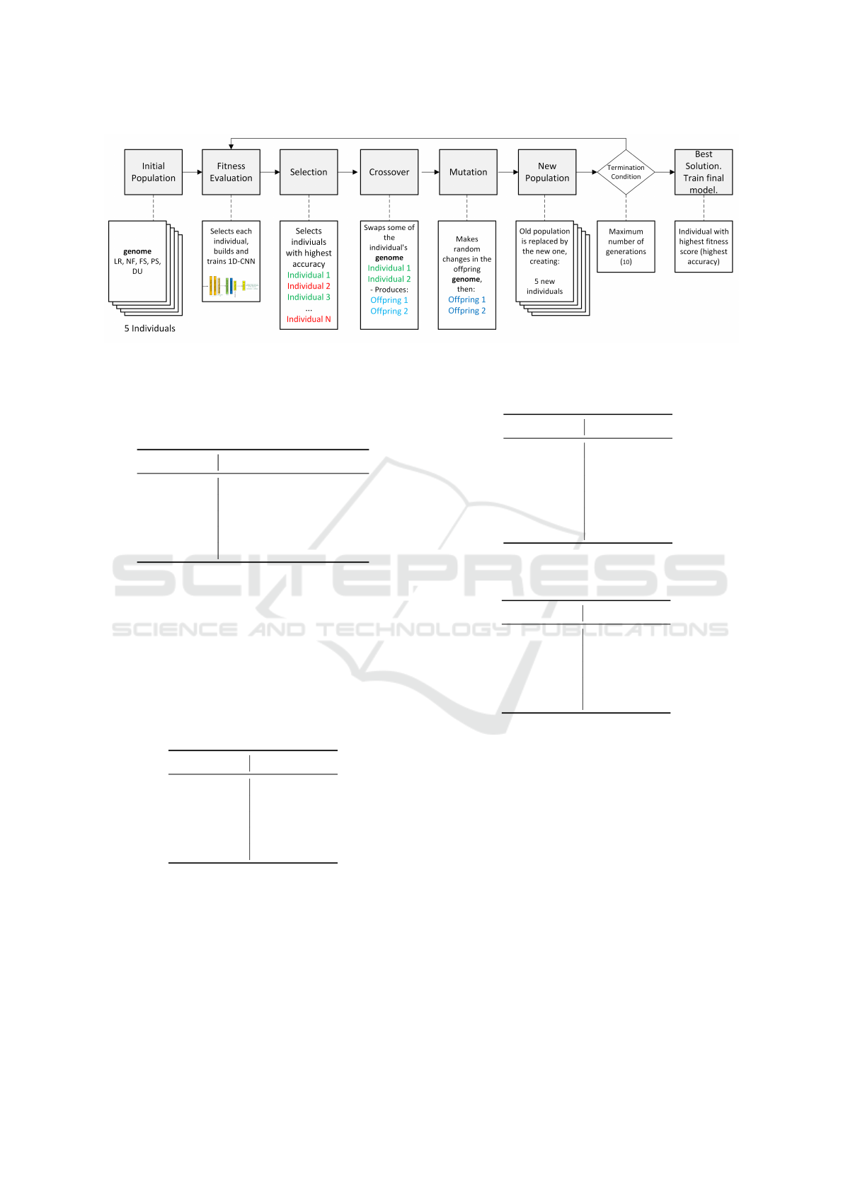
Figure 6: Algorithm for automatic 1D-CNN model optimization.

(DU), batch size (BS), and the option to add (1) or not

(0) an extra dense layer (DL). See Table 8.

Table 8: Genome for the LSTM model.

Parameter Choices

LR 0.0001, 0.001, 0.01, 0.1

LU 32, 64, 128, 256

DU 10, 20, . . . , 100

BS 16, 32, 64, 128

DL 0, 1

After the NAS was run separately for each model

over ten generations, the best hyperparameters were

chosen automatically using the ﬁtness function previ-

ously set, which was the best individual that produced

the highest accuracy. Table 9 shows the hyperparam-

eters automatically selected by the NAS for the 1D-

CNN. These hyperparameters were used to train the

ﬁnal model.

Table 9: Best individual automatically chosen by the NAS

for the 1D-CNN model.

Parameter Best Choice

LR 0.0001

NF 32

FS 4

PS 2

DU 64

Similarly, Table 10 shows the hyperparameters au-

tomatically selected by the NAS for the CNN-VGG

type model, which were additionally used to train the

ﬁnal model.

In a similar way, Table 11 shows the hyperparame-

ters automatically selected by the NAS for the LSTM

model.

Table 10: Best individual automatically chosen by the NAS

for the CNN-VGG type model.

Parameter Best Choice

LR 0.0001

NF 32

NF2 128

FS 3x3

PS 2x2

DU 128

Table 11: Best individual automatically chosen by the NAS

for the LSTM model.

Parameter Best Choice

LR 0.0001

LU 64

DU 70

BS 32

DL Yes

5 EXPERIMENTAL RESULTS

This section presents a discussion of the results ob-

tained from the series of experiments conducted, in-

cluding the data augmentation model’s performance

metrics before and after hyperparameter optimization.

As initially outlined in Section 3.3, our dataset

comprised approximately 487,424 data points for

each class. These data were segmented into 237

blocks per class, each containing 2048 points (size:

2048, 1). To enrich the dataset for training, we aug-

mented it through slight modiﬁcations of existing en-

tries and overlapping blocks, utilizing a stride of 100

data points during segmentation. Consequently, each

new block retained about 95.11% (1948 data points)

from the preceding block and introduced approxi-

Neural Architecture Search for Bearing Fault Classiﬁcation

295

mately 4.89% (100 data points) new information.

As a result, the augmented dataset expanded to ap-

proximately 9.9 million data points, forming around

4860 blocks (size: 2048, 1) per class. This represents

a signiﬁcant increase of over 1930% from the origi-

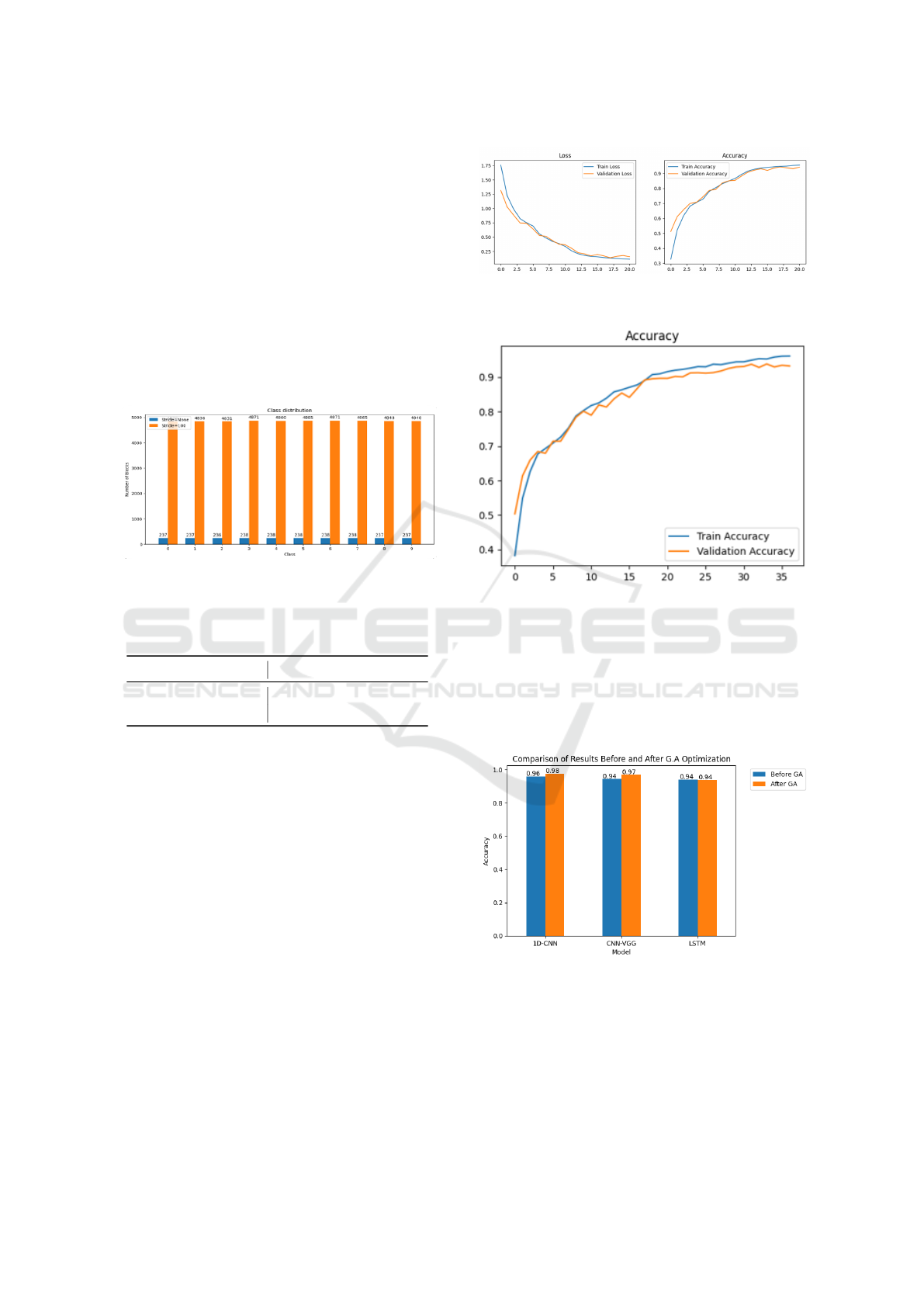
nal dataset size. Refer to Table 12 and Figure 7 for a

comparative bar chart illustrating this expansion.

For experiments requiring 2D input images, we

converted these blocks (size: 2048,1) into Markov

Transition Field (MTF) images (size: 128, 128, 1)

using the MarkovTransitionField class. This conver-

sion was crucial for enabling the application of image-

based machine learning techniques, which typically

require 2D input data.

Figure 7: Number of blocks (2048, 1) created from raw and

augmented data.

Table 12: Comparison of Dataset Sizes Before and After

Augmentation.

Stage Data Points per Class

Original Dataset 487,424

Augmented Dataset Approx. 9.9 million

The training process of the LSTM-manual de-

sign model is depicted in Figure 8, which includes

the loss and accuracy over epochs. As shown, the

model exhibits convergence, with the validation loss

decreasing and validation accuracy increasing in tan-

dem with the training metrics. This indicates a well-

ﬁtting model without signs of overﬁtting or under-

ﬁtting, corroborated by the early stopping mecha-

nism that halted training before the maximum of 50

epochs. This early stopping is particularly evident in

the LSTM-optimized model, whose training and vali-

dation accuracy over epochs is presented in Figure 9.

The steady convergence of training and validation ac-

curacy, along with the early cessation of training, re-

inforces our conﬁdence in the robustness of the model

and the effectiveness of our optimization approach.

Evaluation metrics such as Training Accuracy

(TrainAcc), Test Accuracy (TestAcc), Precision, and

Recall served as the cornerstone for assessing model

performance. Table 13 collates these metrics, con-

trasting models with manually selected hyperparam-

Figure 8: Training and validation loss and accuracy for the

LSTM-manual design model.

Figure 9: Training and validation accuracy for the LSTM-

optimized model.

eters against those reﬁned using Neural Architecture

Search (NAS).

Figure 10 graphically represents the enhancement

in model accuracy post-NAS optimization, visually

underscoring the efﬁcacy of automated hyperparam-

eter tuning.

Figure 10: Comparison of results before and after NAS op-

timization.

All six machine learning models demonstrated

commendable performance, with test accuracies sur-

passing the 0.9400 threshold. Notably, the NAS-

optimized 1D-CNN model reached a test accuracy

pinnacle of 0.9767, a testament to the NAS’s capa-

bility in ﬁne-tuning models for precision tasks. The

ICAART 2024 - 16th International Conference on Agents and Artiﬁcial Intelligence

296

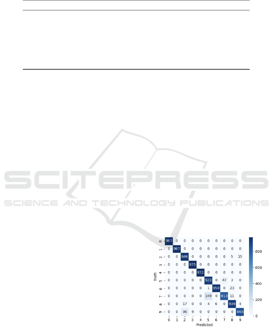
Table 13: Performance Metrics for proposed Models.

Model Train Accuracy Test Accuracy Precision Recall

Manual Design

1D-CNN 0.9859 0.9598 0.9616 0.9598

CNN-VGG 0.9113 0.9448 0.9491 0.9448

LSTM 0.9559 0.9400 0.9399 0.9400

Optimised models with NAS

1D-CNN 0.9949 0.9767 0.9767 0.9720

CNN-VGG 0.9910 0.9697 0.9695 0.9697

LSTM 0.9402 0.9379 0.9381 0.9379

CNN-VGG model followed closely at 0.9697 accu-

racy, reafﬁrming the potential of NAS in enhancing

model discrimination power. This comparison sug-

gests that NAS optimization not only streamlines the

model development process but also potentially ele-

vates performance, particularly for models like 1D-

CNN that inherently beneﬁt from ﬁne-grained param-

eter adjustments.

Conversely, the LSTM models, in both manual

and NAS-optimized variants, manifested marginally

lower performance metrics relative to their counter-

parts. This could be attributed to LSTM’s sensitiv-

ity to hyperparameter settings or its inherent archi-

tecture, which may be less suited for the feature pat-

terns present in the CWRU dataset. Such observations

could imply that while NAS contributes to model re-

ﬁnement, the intrinsic characteristics of each model

architecture play a pivotal role in determining the

overall performance.

The limitations of the analysis are twofold: ﬁrstly,

the optimization process was conﬁned to the pre-

deﬁned parameter space, which, while extensive, may

not encompass the global optimum. Secondly, the

evaluation was conducted exclusively on the CWRU

dataset, which may not fully represent the diverse

conditions encountered in real-world bearing fault di-

agnosis. Future work could extend the parameter

search space and employ datasets with a broader spec-

trum of fault conditions to further validate the robust-

ness of the optimized models.

The confusion matrices presented in Figures 11

and 12 offer a quantitative visual representation of

the classiﬁcation performance for the 1D-CNN model

both prior to and following the application of NAS

for hyperparameter optimization. The matrix prior to

optimization indicates a high degree of classiﬁcation

accuracy for several classes, with off-diagonal zeros

denoting perfect classiﬁcation (100% accuracy) for

those speciﬁc classes. Nevertheless, notable misclas-

siﬁcations were evident, particularly between classes

2 and 9, where 15 instances of class 2 were misclas-

siﬁed as class 9, and between classes 7 and 5, with

149 instances of class 7 being incorrectly classiﬁed

as class 5. This latter misclassiﬁcation rate represents

approximately 15.31% of the total samples for class

7, a signiﬁcant portion that suggests a potential area

for model improvement. The observed errors might

stem from similarities in the feature representations of

these classes that the initial model parameters failed

to disentangle effectively.

After NAS optimization, there was a marked re-

duction in the rate of misclassiﬁcations, exempliﬁed

by the decrease of errors between classes 7 and 5 from

149 to 67 instances. While this still represents a no-

table error rate of 6.89% for class 7, it is a substan-

tial improvement over the pre-optimization rate. This

improvement highlights the effectiveness of NAS in

guiding the model towards a more discriminating pa-

rameter conﬁguration, though the persistence of some

misclassiﬁcations suggests the presence of overlap-

ping features or an intrinsic complexity within the

data that may require further methodological reﬁne-

ments or more sophisticated feature extraction tech-

niques.

Figure 11: Confusion Matrix 1D-CNN prior hyperparame-

ter optimization.

The CNN-VGG and LSTM models also exhibited

misclassiﬁcations, particularly between classes 5 and

7, and 2 and 9. While NAS optimization led to a de-

Neural Architecture Search for Bearing Fault Classiﬁcation

297

Figure 12: Confusion Matrix 1D-CNN following hyperpa-

rameter optimization using NAS.

crease in these errors, the LSTM model showed only

a marginal improvement, hinting at the possibility of

architectural constraints or the need for more targeted

hyperparameter tuning speciﬁc to LSTM’s temporal

processing capabilities.

These results underscore the importance of con-

sidering both model architecture and optimization

strategies in tandem. They also highlight the potential

for a more comprehensive approach to data handling

and preprocessing to alleviate class confusion. Future

work should thus focus on addressing these remain-

ing challenges through advanced optimization tech-

niques, data enrichment strategies, or even exploring

alternative model architectures to achieve a ﬁner gran-

ularity in fault classiﬁcation.

In the ﬁeld of rolling-bearing fault diagnosis, re-

cent research has employed a variety of techniques,

as illustrated in Table 14. The models proposed in

this study, evaluated using the CWRU dataset within

a 10-class experimental framework, demonstrate sig-

niﬁcant achievements in a more intricate classiﬁcation

scenario compared to other studies.

For example, the VI-CNN method (Hoang and

Kang, 2019) and the MTF-CNN model (Wang et al.,

2022b) both achieved 100% accuracy, while the

STFT-CNN (Pham et al., 2020) reached 99.4% ac-

curacy; however, these models were tested within a

simpler 4-class fault classiﬁcation system. Likewise,

the CNNEPDNN (Li and Ji, 2019) model exhibited a

high accuracy of 97.85%, but within a 10-class con-

text.

Contrastingly, our NAS-optimized 1D-CNN

model attained an accuracy of 97.67% in the more

challenging 10-class setup. This performance is

particularly notable given the increased complexity

and diversity of fault types being classiﬁed. This

suggests that our methodology, while comparable in

accuracy to methods tested in less complex scenarios,

demonstrates robustness and effectiveness in more

nuanced classiﬁcation tasks. Therefore, our approach

not only meets the high standards established by

existing techniques but also expands the potential

for precise fault classiﬁcation in more demanding

scenarios. Refer to Table 14 for a detailed compar-

ison of these methods. This analysis highlights the

signiﬁcance and efﬁcacy of the models developed

in this study, especially regarding their capability to

discriminate between a wider range of fault classes.

Table 14: Model’s Performance from other studies. The

methods include VI-CNN (Hoang and Kang, 2019), STFT-

CNN (Pham et al., 2020), IDSCNN (Li et al., 2017),

CNNEPDNN (Li and Ji, 2019), MTF-CNN (Wang et al.,

2022b), LSTM (Wang et al., 2022b), and Compact 1D-CNN

(Chuya-Sumba et al., 2022), 1D-CNN (Wang et al., 2022a),

LSTM (Wang et al., 2022a).

Method Classes Accuracy (%)

VI-CNN 4 100

STFT-CNN 4 99.4

IDSCNN 10 93.84

CNNEPDNN 10 97.85

MTF-CNN 4 100

LSTM 4 79.8

Compact 1D-CNN 7 93.2

1D-CNN 7 100

LSTM 7 95

Building upon the comparative analysis, Table 14

directly showcases the performance accuracy of the

models developed in our study, evaluated over ten

classes. This table provides a clear perspective on

how our proposed models perform in relation to the

benchmarks set by the studies mentioned previously.

It offers a detailed view of our models’ effective-

ness in the more complex 10-class fault classiﬁcation,

highlighting their capabilities and contributions to the

ﬁeld of fault diagnosis using machine learning tech-

niques.

Table 15: Model’s Performance from proposed models.

Model Classes Accuracy

Manual Design

1D-CNN 10 0.9598

CNN-VGG 10 0.9448

LSTM 10 0.9400

Optimised with NAS

1D-CNN 10 0.9767

CNN-VGG 10 0.9697

LSTM 10 0.9379

ICAART 2024 - 16th International Conference on Agents and Artiﬁcial Intelligence

298

Comparatively, the proposed 1D-CNN optimized

with NAS demonstrated a high accuracy of 0.9767 de-

spite being evaluated across ten classes, which inher-

ently present more complex classiﬁcation challenges.

Similarly, the other models proposed in this study

also demonstrated a competitive performance, with

a minimum accuracy of 0.9400. This reinforces the

efﬁcacy of the proposed models, data augmentation,

and NAS optimization for the classiﬁcation of bear-

ing faults using vibration data, even in more complex

scenarios.

6 CONCLUSION

The research presented in this study provided signiﬁ-

cant insights into the use of machine learning models

for bearing fault classiﬁcation using vibration data,

with particular emphasis on the performance of 1D-

CNN, CNN-VGG, and LSTM models. Additionally,

the study underscored the potential of data augmenta-

tion techniques and NAS in improving model perfor-

mance.

Data augmentation proved beneﬁcial, expanding

the dataset and leading to improved model training.

The application of NAS for hyperparameter op-

timization was successful in boosting model perfor-

mance. NAS enabled an automated and efﬁcient ex-

ploration of a larger parameter space, uncovering op-

timal hyperparameters. This approach notably im-

proved the validation accuracies of the 1D-CNN and

CNN-VGG type models optimized with NAS. The

NAS-optimized 1D-CNN model achieved the highest

test accuracy, though some models faced challenges

in differentiating between certain classes, indicating

room for further improvement.

The comparison of results demonstrated that while

other studies have achieved high accuracies, the meth-

ods and models proposed in this study displayed ex-

cellent results in more complex classiﬁcation scenar-

ios. This suggests that the combination of data aug-

mentation, machine learning models, and NAS opti-

mization can offer more reliable and high-performing

solutions for bearing fault classiﬁcation using vibra-

tion data.

In summary, the conducted study effectively

demonstrated the utilization and integration of ma-

chine learning models, data augmentation, and NAS

for bearing fault classiﬁcation using vibration data.

This integration represents a signiﬁcant step forward

in the technology used for fault detection and classi-

ﬁcation. The 1D-CNN NAS-optimized model exhib-

ited superior performance, demonstrating the poten-

tial of this integrated approach, suggesting that a more

simplistic model (1D-CNN) can achieve better results

for addressing this problem (bearing fault classiﬁca-

tion) than the use of more complex models (CNN-

VGG and LSTM) that require additional data trans-

formation (1-dimensional into 2-dimensional). Nev-

ertheless, the scope for further reﬁnement remains.

For future work, we plan to increase the size of

the population and the number of generations in the

genetic algorithm (GA) used in the Neural Architec-

ture Search (NAS) to further improve the performance

of the proposed models. Addressing the challenges in

class distinction within bearing fault classiﬁcation re-

mains a priority. Additionally, we plan to include a

wider range of datasets to enhance the accuracy and

generalizability of the models. Lastly, the ultimate

goal is to apply these models in real-world scenarios,

which would provide valuable insights into their per-

formance in diverse operational environments.

This research contributes to the existing body of

knowledge in the ﬁeld, and the ﬁndings present a po-

tential impact on the industry, particularly in how vi-

bration data and machine learning can address bear-

ing fault classiﬁcation in practical settings. Moreover,

the insights gained from this research can be applied

to other predictive maintenance technologies, such as

ultrasound analysis, which faces similar challenges.

ACKNOWLEDGEMENTS

This work was supported, in part, by Science

Foundation Ireland grant 13/RC/2094 P2 and co-

funded under the European Regional Development

Fund through the Southern & Eastern Regional

Operational Programme to Lero - the Science

Foundation Ireland Research Centre for Software

(www.lero.ie). The authors also thank Eastway Re-

liability (https://eastwaytech.com) for supporting this

work.

REFERENCES

Ahmed, A. A., Darwish, S. M. S., and El-Sherbiny, M. M.

(2020). A novel automatic cnn architecture design

approach based on genetic algorithm. In Hassanien,

A. E., Shaalan, K., and Tolba, M. F., editors, Pro-

ceedings of the International Conference on Advanced

Intelligent Systems and Informatics 2019, pages 473–

482, Cham. Springer International Publishing.

Chuya-Sumba, J., Alonso-Valerdi, L.M., and Ibarra-Zarate,

D. (2022). Deep-learning method based on 1d convo-

lutional neural network for intelligent fault diagnosis

of rotating machines. Applied Scences, 12(4):2158.

Neural Architecture Search for Bearing Fault Classiﬁcation

299

CWRU-Dataset. (2023). Cwru bearing data center, case

western reserve university. https://engineering.case.

edu/bearingdatacenter/. Accessed: 24 October 2023.

Elsken, T., Metzen, J. H., and Hutter, F. (2019). Neural

architecture search: A survey.

Faouzi, J. et al. (2017). Markovtransitionﬁeld.

2017-2021, Johann Faouzi and all pyts con-

tributors. Available at: https://pyts.readthedocs.

io/en/stable/ modules/pyts/image/mtf.html#

MarkovTransitionField (Accessed: 30 July 2023).

Goodfellow, I., Bengio, Y., and Courville, A. (2016). Deep

learning. MIT press.

Hoang, D.-T. and Kang, H.-J. (2019). Rolling element bear-

ing fault diagnosis using convolutional neural network

and vibration image. Cognitive Systems Research,

53:42–50.

Hochreiter, S. and Schmidhuber, J. (1997). Long short-term

memory. Neural computation, 9(8):1735–1780.

Houreh, Y., Mahdinejad, M., Naredo, E., Dias, D. M., and

Ryan, C. (2021). Hnas: Hyper neural architecture

search for image segmentation. In ICAART (2), pages

246–256.

ISO (2015). Bearing damage and failure analy-

sis, p.8. https://www.iso.org/obp/ui/en/#iso:std:iso:

15242:-1:ed-2:v1:en. Accessed: 24 October 2023.

Laredo, D., Qin, Y., Sch

utze, O., and Sun, J.-Q. (2019).

Automatic model selection for neural networks.

Li, H. and Ji (2019). Bearing fault diagnosis with a fea-

ture fusion method based on an ensemble convolu-

tional neural network and deep neural network. Sen-

sors, 19:2034.

Li, S., Liu, G., Tang, X., Lu, J., and Hu, J. (2017). An en-

semble deep convolutional neural network model with

improved ds evidence fusion for bearing fault diagno-

sis. Sensors, 17(8):1729.

Li, Z., Liu, F., Yang, W., Peng, S., and Zhou, J. (2022).

A survey of convolutional neural networks: Anal-

ysis, applications, and prospects. IEEE Transac-

tions on Neural Networks and Learning Systems,

33(12):6999–7019.

Liu, J. et al. (2021). Fault prediction of bearings

based on lstm and statistical process analysis. Re-

liability Engineering & System Safety. Available

at: https://www.sciencedirect.com/science/article/pii/

S0951832021001873 (Accessed: 01 June 2023).

Liu, R., Yang, B., Zio, E., and Chen, X. (2018). Artiﬁcial

intelligence for fault diagnosis of rotating machinery:

A review. Mechanical Systems and Signal Processing,

108:33–47.

Montana, D. J. and Davis, L. (1989). Training feedforward

neural networks using genetic algorithms. In Pro-

ceedings of the 11th International Joint Conference

on Artiﬁcial Intelligence - Volume 1, IJCAI’89, page

762–767, San Francisco, CA, USA. Morgan Kauf-

mann Publishers Inc.

Peng, B., Wan, S., Bi, Y., Xue, B., and Zhang, M.

(2020). Automatic feature extraction and construc-

tion using genetic programming for rotating machin-

ery fault diagnosis. IEEE transactions on cybernetics,

51(10):4909–4923.

Pham, M., Kim, J.-M., and Kim, C. (2020). Accurate bear-

ing fault diagnosis under variable shaft speed using

convolutional neural networks and vibration spectro-

gram. Applied Sciences, 10:6385.

Pinedo-Sanchez, L. A., Mercado-Ravell, D. A., and

Carballo-Monsivais, C. A. (2020). Vibration analysis

in bearings for failure prevention using cnn. Journal

of the Brazilian Society of Mechanical Sciences and

Engineering, 42(12):628.

Romanssini, M., de Aguirre, P. C. C., Compassi-Severo, L.,

and Girardi, A. G. (2023). A review on vibration mon-

itoring techniques for predictive maintenance of rotat-

ing machinery. Eng, 4(3):1797–1817.

Sakib, N. and Wuest, T. (2018). Challenges and opportuni-

ties of condition-based predictive maintenance: a re-

view. Procedia cirp, 78:267–272.

Scanlan, T. (2023). Deep convolutional neural network on

cifar-10 dataset. Lecture slides in Deep Learning for

Image Classiﬁcation. Machine Vision Module.

Simonyan, K. and Zisserman, A. (2014). Very deep con-

volutional networks for large-scale image recognition.

arXiv preprint arXiv:1409.1556.

SKF-Group. (2017). Bearing damage and failure analysis,

p.8. https://www.skf.com/binaries/pub12/Images/

0901d1968064c148-Bearing-failures---14219\

2-EN\ tcm\ 12-297619.pdf. Accessed: 30 Septem-

ber 2022.

SKF-Group. (2023). Bearing rating life. https:

//www.skf.com/sg/products/rolling-bearings/

principles-of-rolling-bearing-selection/

bearing-selection-process/bearing-size/

size-selection-based-on-rating-life/

bearing-rating-life. Accessed: 24 October 2023.

Wang, H., Sun, W., He, L., and Zhou, J. (2022a). Rolling

bearing fault diagnosis using multi-sensor data fusion

based on 1d-cnn model. Entropy, 24(5):573.

Wang, M., Wang, W., Zhang, X., and Iu, H. H.-C. (2022b).

A new fault diagnosis of rolling bearing based on

markov transition ﬁeld and cnn. Entropy, 24(6):751.

Xia, M., Li, T., Xu, L., Liu, L., and De Silva, C. W.

(2017). Fault diagnosis for rotating machinery us-

ing multiple sensors and convolutional neural net-

works. IEEE/ASME transactions on mechatronics,

23(1):101–110.

Yan, J., Kan, J., and Luo, H. (2022). Rolling bearing fault

diagnosis based on markov transition ﬁeld and resid-

ual network. Sensors, 22(10):3936.

ICAART 2024 - 16th International Conference on Agents and Artiﬁcial Intelligence

300