Information Theoretic Deductions Using Machine Learning with an

Application in Sociology

Arunselvan Ramaswamy

1 a

, Yunpeng Ma

, Stefan Alfredsson

1 b

, Fran Collyer

2 c

and

Anna Brunstr

1 d

Dept. of Mathematics and Computer Science, Karlstad University, Sweden

School of Humanities and Social Inquiry, University of Wollongong, Australia

anna.brunstrom@kau.se

Keywords:

Conditional Entropy, Binary Classiﬁcation, Information Theory, Supervised Machine Learning,

Automated Data Mining, Machine Learning in Sociology.

Abstract:

Conditional entropy is an important concept that naturally arises in ﬁelds such as ﬁnance, sociology, and

intelligent decision making when solving problems involving statistical inferences. Formally speaking, given

two random variables X and Y , one is interested in the amount and direction of information ﬂow between X

and Y. It helps to draw conclusions about Y while only observing X . Conditional entropy H(Y |X) quantiﬁes

the amount of information ﬂow from X to Y . In practice, calculating H(Y |X) exactly is infeasible. Current

estimation methods are complex and suffer from estimation bias issues. In this paper, we present a simple

Machine Learning based estimation method. Our method can be used to estimate H(Y |X) for discrete X and

bi-valued Y. Given X and Y observations, we ﬁrst construct a natural binary classiﬁcation training dataset. We

then train a supervised learning algorithm on this dataset, and use its prediction accuracy to estimate H(Y |X ).

We also present a simple condition on the prediction accuracy to determine if there is information ﬂow from X

to Y. We support our ideas using formal arguments and through an experiment involving a gender-bias study

using a part of the employee database of Karlstad University, Sweden.

1 INTRODUCTION

Conditional entropy is an information theoretic term

that quantiﬁes the amount of information required to

describe one random variable, given that the value of

another random variable is known. It naturally arises

in many scenarios and calculating its value is often

very useful. Consider the following – given the global

ﬁnancial trend, e.g., Dow Jones Industrial Average or

S&P 500 index, it is interesting to predict trends in a

speciﬁc Company, say company C . Such an analysis

would indicate if C is a market sensitive or a mar-

ket leading company. Also, the degree and direction

of information transfer between various stock market

indices is important (Dimpﬂ and Peter, 2013) (Dar-

bellay and Wuertz, 2000). This is often studied us-

ing a quantity related to conditional entropy called the

https://orcid.org/0000-0001-7547-8111

https://orcid.org/0000-0003-0368-9221

https://orcid.org/0000-0002-9877-6645

https://orcid.org/0000-0001-7311-9334

transfer entropy.

Let us suppose that random variable X represents

the evolution of the global stock market, and that ran-

dom variable Y represents the evolution of company

C . The conditional entropy under question is

H(Y |X) = −

∑

x∈X

∑

y∈Y

y|x

log p

y|x

, (1)

where p

= P(X = x), p

y|x

= P(Y = y|X = x), X and

Y are the supports of random variables X and Y , re-

spectively. For the sake of simplicity we have as-

sumed that X and Y are discrete valued (and even

countable). Suppose, they are continuous then the

summations in (1) are replaced by integrals. H(Y |X)

quantiﬁes the amount of information needed to de-

scribe Y , given that X is known. It can be shown that

0 ≤ H(Y |X) ≤ H(Y ), where H(Y ) = −

∑

y∈Y

log p

is the entropy of Y, the amount of uncertainty in Y.

If H(Y |X) = 0, then Y can be fully determined by

X, e.g., when Y = X

. X and Y are independent iff

H(Y |X) = H(Y ) (MacKay et al., 2003). Finally, note

that conditional entropy is an asymmetric quantity –

320

Ramaswamy, A., Ma, Y., Alfredsson, S., Collyer, F. and Brunström, A.

Information Theoretic Deductions Using Machine Learning with an Application in Sociology.

DOI: 10.5220/0012371600003654

Paper published under CC license (CC BY-NC-ND 4.0)

In Proceedings of the 13th International Conference on Pattern Recognition Applications and Methods (ICPRAM 2024), pages 320-328

ISBN: 978-989-758-684-2; ISSN: 2184-4313

H(Y |X) only considers the information ﬂow from X

to Y. Let us circle back to the stock market scenario.

If H(Y |X) = 0, then company C follows the global

trend to the highest degree. The value of H(Y |X) is

inversely proportional to the degree of dependency of

C on the global trend.

In practice, calculating the conditional entropy is

infeasible as it requires complete knowledge of the

joint and marginal probability distributions of X and

Y . Hence, it is often estimated using X and Y observa-

tions (Pham, 2004). Such data-driven estimators are

often sophisticated, while suffering from signiﬁcant

estimation biases (Beirlant et al., 1997).

In the ﬁeld of computer security, a side channel

attack is an attack that is based on extra information

that can be gathered owing to the fundamental way in

which a computer algorithm is implemented (Golder

et al., 2019). In order to prevent side-channel attacks,

security analysts must ascertain the amount of data,

which when collected, can be used to compromise a

computer. Let us deﬁne X to be the random variable

associated with the gathered data – the “side-channel

information”. Let us also deﬁne the two valued ran-

dom variable Y as equalling 1 if the security is com-

promised, and 0 otherwise. Then H(Y |X) quantiﬁes

how much of X must be observed in order to accu-

rately determine Y . Again, calculating H(Y |X) ex-

actly is infeasible. Machine Learning was recently

used to skirt around this (Drees et al., 2021) (Gupta

et al., 2022). However, these works are preliminary

and empirical without formal backing. In any case

they do not attempt to estimate conditional entropy or

draw information theoretic conclusions.

Our Contributions. We present a Machine Learning

based easy-to-implement method to estimate the con-

ditional entropy H(Y |X), where Y is a bi-variate ran-

dom variable and X is discrete valued. This estimate

is used to measure the degree of dependency of Y on

X. Given observations of X and Y , we discuss how to

transform the problem of estimating the conditional

entropy to a supervised learning problem. We then

use the prediction accuracy of the supervised learn-

ing algorithm to estimate the conditional entropy. We

present sufﬁcient conditions on the accuracy of the

learning algorithm for guaranteed information ﬂow

from X to Y. We support our ideas through formal ar-

guments and experiments on real datasets.

1.1 Conditional Entropy in Sociology:

A Data-Driven Approach

Companies and organizations aim to ensure their male

and female employees are equally represented, that

their policies are not skewed towards one gender.

Conditional entropy plays an essential role when ana-

lyzing the current state of affairs with respect to gen-

der equality in these organizations. Here, we present

an ML-based approach for such an analysis. First,

the employee database is used to create a supervised

learning (classiﬁcation) dataset. There is one input in-

stance corresponding to each employee. It only con-

tains gender neutral information such as date of birth,

salary, position, etc. Gender revealing information

such as names, gender, etc., are excluded. The input

instances are labeled using their gender – 0 for female

and 1 for male. We are therefore in the setting of bi-

nary classiﬁcation. We use X to represent the random

variable associated with the input, and Y to represent

the class random variable.

If the gender does not play a role in hiring and

subsequent career development, then one cannot re-

liably predict the gender Y merely using the gender

neutral information X, such as the title and salaray. In

the parlance of information theory, H(Y |X) = H(Y ).

On the other hand, suppose there is gender bias, then

H(Y |X) < H(Y ). In this paper, we call a dataset gen-

der biased when the genders are unequally repre-

sented (gender plays a role in hiring, career devel-

opment, etc.) when H(Y |X) < H(Y ). As explained

earlier, we present a supervised learning approach to

estimating H(Y |X ), and checking if H(Y |X) < H(Y ).

The gender inequality problem is very well stud-

ied in literature, see, e.g., (Heiberger, 2022). Also,

ML tools have been been previously used to em-

pirically study problems in sociology, e.g., (Zajko,

2022) (Molina and Garip, 2019). To the best of our

knowledge, this is the ﬁrst time in literature, wherein

ML is used within the framework of statistical infer-

ence to answer a sociological question, in particu-

lar a gender-bias question. Further, the framework is

backed by formal theory.

Here is another scenario where our methodology

is useful. Let us suppose that a vast region is ﬂooded.

After emergency relief operations, the responsible

government committee must formulate a plan to allo-

cate resources and funds for the long-term rebuilding

process. For the sake of simplicity, let us suppose that

the region can be divided into neighborhoods – each

consisting of groups of houses, one or more commu-

nity centers, commercial buildings, schools and hos-

pitals. The committee must allocate resources at the

“neighborhood level”. Resource allocation must be

done in a fair and equitable manner, proportional to

the losses incurred by the neighborhood. Further, the

associated timelines, e.g., to release funds, must fa-

cilitate immediate and equitable relief. The plan must

not be inﬂuenced by the political orientation, racial

identity or afﬂuence of any given neighborhood.

Information Theoretic Deductions Using Machine Learning with an Application in Sociology

321

Given a proposal, how does one go about check-

ing if the plan satisﬁes the above mentioned equity

constraints? Traditionally, a human expert evaluates

the plan, the draft is then amended based on the feed-

back and sent for reevaluation, this process is re-

peated a few times. The framework presented in

this paper can hasten the feedback loop through the

introduction of an automated bias checking routine.

For plan evaluation, we ﬁrst create a dataset contain-

ing datapoints with the following information on the

neighborhoods: general information about a neigh-

borhood (e.g., number of houses, schools, average

household income, etc.), information on ﬂood dam-

age (e.g., fraction of the neighborhood affected, loss

to critical services, etc.), and information on ﬂood

relief (e.g., allocated resources and funds, timeline,

etc.). The data should not include information that

must be disregarded during planning – neighborhood-

racial-identity, afﬂuence, etc. There is one datapoint

corresponding to every neighborhood in the ﬂooded

region.

A Machine Learning (ML) algorithm is then

trained on the dataset to predict, e.g., the majority po-

litical orientation of neighborhoods. If the prediction

accuracy is high enough, then our analysis shows that

the draft is biased. Put simply, the predictor should

not perform better than guessing, when predicting the

neighborhood-political-orientation for a draft to be

deemed unbiased. From an information theoretic per-

spective, a high accuracy indicates that there is some

information regarding political orientation present in

the data. Note that the bias may be positive or neg-

ative. On the other hand, suppose the prediction ac-

curacy is low (accuracy corresponding to guessing),

then the draft is probably fair. Although the ML based

bias predictor can provide as assessment within a mat-

ter of hours, if not minutes, it does not have the ca-

pacity to assess the cause for the bias. The draft may

be passed to an expert for feedback only if the ML

predictor detects a bias, thus saving valuable time and

effort.

2 FORMAL PROBLEM SETUP

AND OUR APPROACH

Today, enormous data on individuals, anonymized

and otherwise, is readily available in the public do-

main. Decision making bodies utilize this data, ana-

lyze them, and base important decisions on conclu-

sions based on these analyses. Social biases, e.g.,

gender and race, intrinsic to the data, affect the deci-

sion making process. Information theoretic quantities

like conditional entropy play a pertinent role in quan-

tifying the biases in the aforementioned databases.

However, these quantities are hard to estimate. In

this paper, we propose a supervised learning based

framework to solve the problem of estimating the

conditional entropy of information extracted from

databases. We propose a novel framework based on

ML and Statistics. We stick to the parlance of gender

bias to illustrate our ideas. It must however be noted

that they can be readily extended to study other types

of biases and information ﬂows.

Machine Learning (ML) is the study of algorithms

that self-improve at performing tasks only through

data (Bishop and Nasrabadi, 2006) (Goodfellow et al.,

2016) (Hastie et al., 2009). Supervised learning is an

important ML paradigm where the algorithm learns

to perform tasks by emulating examples. Mathemat-

ically speaking, a supervised learning algorithm tries

to learn an unknown map Y : X → Y , where X and

Y are the input and output spaces respectively, us-

ing example data called training data, represented by

the set D = {(x

,Y (x

)) | x

∈ X }

1≤n≤N

for some

1 ≤ N < ∞. A supervised learning algorithm A learns

a map Y

, using D, that approximates the unknown

map Y. Speciﬁcally, it ﬁnds Y

that minimizes pre-

diction errors on D.

We are given X and Y observations

{(x

)}

1≤n≤N<∞

, where X is discrete-valued and Y

is bi-valued. This observation set naturally translates

to the training dataset for a binary classiﬁcation

algorithm A. Training A yields a proxy map Y

(X)

and an associated prediction accuracy. It is then

used to (a) estimate the required conditional entropy

H(Y |X), and (b) assert whether H(Y |X) < H(Y ) in

order to comment on the dependency of Y on X.

In the context of a gender bias study, X represents

all perceived gender neutral information and Y the

gender information, 0 for female and 1 for male. The

observation data/training data is typically obtained

from a database - the starting point for our analysis.

The prediction accuracy is used to decide if there is

gender information contained in X, if the database

is gender biased. Intuitively speaking, we draw this

conclusion based on whether the prediction accuracy

is signiﬁcantly better than guessing. If so, then A is

able to exploit a possibly hidden pattern in the data

with respect to gender. A human expert may now be

summoned to carefully check the data in order to ﬁnd

the source of the perceived gender bias. Finally, we

also comment on the degree of bias by estimating the

required conditional entropy. It must be noted that

the exact classiﬁcation algorithm used in the analysis

depends on the nature of the data X. Typically, one

works with an ensemble of algorithms.

ICPRAM 2024 - 13th International Conference on Pattern Recognition Applications and Methods

322

Our Approach. Let us suppose that we are given a

database containing datapoints on people. Addition-

ally, we are given the gender information for each dat-

apoint. From this we construct a classiﬁcation dataset

D = {(x

) | 1 ≤ n < ∞}, where x

is the supposed

gender neutral information regarding the n

individ-

ual, extracted from the database, and y

is the corre-

sponding gender. We let y

= 0 for female and y

= 1

for male. Let X be the random variable associated

with the perceived gender neutral information, and Y

be the gender random variable. Deﬁne,

# of males in the database ∨ # of females in the database

|D|

(2)

where ∨ denotes the max operator. We train an en-

semble E of binary classiﬁcation algorithms using D.

Let us suppose that there is at least one algorithm

A ∈ E with an accuracy that is strictly greater than

p. Then, we argue that D is gender biased. In partic-

ular, we show that the conditional entropy H(Y | X) <

H(Y ). Recall that H(Y | X ) represents the amount

of information required to describe the outcome of

Y given that the value of X is known. It is known

that H(Y | X) is at most H(Y ), i.e., H(Y | X) ≤ H(Y ).

Suppose X does not contain any information about

Y , X and Y are independent random variables, then

H(Y | X) = H(Y ). Hence, H(Y | X ) < H(X) indicates

that X contains gender information, it can describe the

outcome of Y .

On the other hand, suppose that none of the clas-

siﬁers in the ensemble have an accuracy better than p,

then it is very likely that H(Y | X) = H(Y ). From a

theoretical standpoint, the Baye’s classiﬁer is the op-

timal classiﬁcation algorithm, in that it has the high-

est accuracy. We may replace our ensemble with the

Baye’s classiﬁer in order to be sure. The only issue

is that the Baye’s classiﬁer is computationally infea-

sible for most classiﬁcation problems. To summarize

our approach, we create a classiﬁcation dataset from

the database entries and solve the gender classiﬁca-

tion problem. We show that high accuracy, speciﬁ-

cally better than guessing, is indicative of a gender

bias in the dataset.

3 INFORMATION THEORETIC

BACKING FOR GENDER BIAS

DETECTION USING

CLASSIFICATION

In the parlance of machine learning, X is called the

feature random vector and Y is called the class ran-

dom variable. In order to detect gender bias in D, one

typically estimates the mutual information I(X,Y ),

which is related to conditional entropy through the

following formula:

I(X,Y ) = H(Y ) − H(Y | X) = H(X) − H(X | Y ) (3)

where H(X) and H(Y ) are the entropies of X and Y re-

spectively, H(X | Y) and H(Y | X ) are the conditional

entropies of X given Y and Y given X, respectively.

The mutual information I(X ,Y ) quantiﬁes the infer-

ence that can be drawn regarding one random vari-

able by observing the other. Mutual information is

symmetric – I(X ,Y ) = I(Y,X) – and always positive

– I(X,Y ) ≥ 0.

When I(X,Y ) = 0, no information can be drawn

regarding Y by observing X. Due to the symmetric na-

ture of mutual information a similar statement can be

made by swapping X and Y in the previous sentence.

We are, however, only interested in the former and

we will stick to it. From (3) it therefore follows that

H(Y ) = H(Y | X). Simply put, observing X does not

reduce the uncertainty in Y . On the other hand, when

I(X,Y ) > 0, information regarding Y can be inferred

by observing X. The higher the value, the better the

inference. Again from (3), we get the equivalent con-

dition that H(Y ) > H(Y | X). Colloquially speaking,

observing X has reduced the uncertainty in Y . Sup-

pose H(Y | X) = 0, then I(X,Y ) takes the maximum

possible value of H(Y ), and Y is fully determined by

observing X.

Let us circle back to the problem at hand. We

are interested in quantifying the gender inference

(describing Y ) through only observing X (the per-

ceived gender neutral information regarding an in-

dividual extracted from the database). If we show

that I(X,Y ) = 0, or equivalently that H(Y | X) =

H(Y ), then gender inference is not possible, and the

database is not gender biased. If, on the other hand,

we show that I(X,Y ) > 0, or equivalently that H(Y |

X) < H(Y ), then the gender can be fully or partially

inferred, and the database is gender biased. Hence,

the ﬁrst order of business is to estimate these entropy

quantiﬁers.

Instead of using complex biased entropy estima-

tors from literature, we propose solving an associ-

ated classiﬁcation problem. We propose predicting

the gender of individuals Y solely using X. This yields

a natural binary classiﬁcation problem, and a natural

training dataset D. We show that using D to effec-

tively train a classiﬁer (Machine Learning model) to

predict the gender with high accuracy for any individ-

ual from the database is an indicator of gender bias.

Our Contribution. We show H(Y | X) < H(Y ) when

a binary classiﬁer, trained on D, has an accuracy that

is strictly greater than p (recall the deﬁnition of p

Information Theoretic Deductions Using Machine Learning with an Application in Sociology

323

from (2)). In effect, showing that an accuracy strictly

greater than p implies that the database is gender bi-

ased. We also analyze the scenario when the classiﬁer

used is optimal – Bayes classiﬁer. In the course of this

analysis, we estimate H(Y | X ) and H(Y ).

Baye’s classiﬁer is the theoretical optimal, in

that, it has the highest accuracy among all classiﬁers

trained on D. However, it requires full knowledge of

the underlying population distribution that generated

the data in the database, and consequently D itself.

As there is no access to the population distribution,

we resort to other feasible albeit suboptimal classi-

ﬁers that only require D. The dataset D is assumed

to be generated from the joint unknown distribution

on (X,Y ) - also known as the population distribution

- through repeated and independent sampling.

3.1 Entropy of a Gender Guessing

Algorithm

First, we deﬁne the following notations: p

= P(X =

x), p

= P(Y = y) and p

y|x

= P(Y = y | X = x).

These together, deﬁne the required population distri-

bution. Without loss of generality, we assume that

the database contains at least as many male represen-

tatives as female ones. Since we assumed that D is

generated by the underlying population distribution,

provided it is also large, we have P(Y = 1) ≈ p and

P(Y = 0) ≈ 1 − p, where p is deﬁned in (2). Now,

consider a randomized classiﬁer G (gender guess-

ing algorithm) that predicts with probability p that a

given query instance x belongs to class-1, and pre-

dicts class-0 with probability 1 − p. In effect, G does

not truly consider x when predicting gender. If we

associate the random variable Y

(x) with the predic-

tion of G, then Y

(x) = 1 with probability p and

(x) = 0 with probability 1 − p. Note that x is an

instance/realization of X.

Let p

y|x

= P(Y

(x) = y | X = x). Then, the con-

ditional entropy,

H(Y

(X)|X) = −

∑

x∈X

∑

y∈Y

y|x

log p

y|x

where X is the support of X – the set of all possible

values of X – and Y = {0,1}. Since G does not truly

consider X during prediction, we have that p

y|x

= p

for all x ∈ X and y ∈ Y , and the above equation be-

comes

H(Y

(X)|X) = −

∑

x∈X

∑

y∈Y

log p

= H(Y ).

This is not surprising since G has not used X for pre-

diction. Suppose D is not gender biased, then G is the

optimal predictor. In other words, where one cannot

do better than guessing, and X is useless in predicting

the gender.

3.2 Baye’s Classiﬁer B when D Is not

Gender Biased

One sufﬁcient condition for D to be gender unbiased

is when X and Y are uncorrelated, when p

= p

y|x

for

x ∈ X and y ∈ Y . The Baye’s classiﬁer is given by the

following deterministic mapping from X onto Y :

x 7→ argmin

y∈Y

ℓ(0,y)p

0|x

+ ℓ(1,y)p

1|x

, (4)

where ℓ(y

) = 1 when y

̸= y

and 0 otherwise,

∈ Y . ℓ is called the 0-1 loss function, it penal-

izes a wrong prediction by 1. Baye’s predictor is a

mapping that minimizes the average loss, where the

average is taken with respect to the population distri-

bution. When using the 0-1 loss function, minimiz-

ing the average loss is equivalent to maximizing the

average accuracy, again the average is taken with re-

spect to the population distribution. One can use (4) to

show that the Baye’s classiﬁer B predicts 0 at x when

1|x

< p

0|x

, and 1 otherwise. Hence, (4) is equivalent

x 7→ argmax

y∈Y

y|x

Since we assumed that X and Y are uncorrelated, B

reduces to the constant map

x 7→ argmax

y∈Y

We assumed without loss of generality that p

≥ p

hence B predicts that every query instance x belongs

to class-1. The Bayes classiﬁer B becomes the

majority classiﬁer, it classiﬁes every query instance

as the majority class – class-1 in our case. B has an

accuracy of p (= p

), since it is correct only on query

instances that are male. The associated prediction

random variable Y

(x) = 1 with probability 1 for all

x ∈ X . Further, P(Y

(x) is the correct label for x) =

p. Deﬁne a random variable Z(X) =

1(Y

(X) is the correct label for X), then EZ(X) = p.

Note that 1 is the indicator random variable whose

outcome is always 0 or 1. It is 1 only when

(x) is the correct label for x and 0 otherwise. Z(X)

is fully determined by X, Z(X) = 1 when X belongs

to class-1 (male) and Z(X ) = 0 otherwise. Therefore,

Z(X) is 1 with probability p (= p

) and 0 with

ICPRAM 2024 - 13th International Conference on Pattern Recognition Applications and Methods

324

probability 1 − p (= p

). Its entropy is given by

H(Z(X)) = −

∑

z∈{0,1}

P(Z(X) = z)logP(Z(X) = z)

= −(p log p + (1 − p)log(1 − p))

= −(p

log p

+ p

log p

) = H(Y ).

(5)

The uncertainty associated with predicting the gender

correctly is equal to the uncertainty in the gender it-

self. Since Z(X) is fully determined by X, it is clear

that the knowledge of X has not reduced the uncer-

tainty in gender prediction. Therefore, we can con-

clude that B has not extracted any gender information

from X, spurious or otherwise.

3.3 Entropy of a Classiﬁcation

Algorithm A

Intuitively speaking, the database is gender biased

if the gender of an individual can be determined

with high accuracy, using only the perceived gender

neutral information that can be extracted from the

database. The higher the bias, the better the gender

determination, the easier the gender prediction. Let

us suppose that we have a classiﬁcation algorithm

A that is trained on D to predict the gender variable

Y . Let Y

(X) be the prediction random variable

obtained by training A on D. It is the best approxi-

mation of Y found by A using D. Deﬁne p(A,x))

P(Y

(X) predicts the class of X correctly|X = x).

Suppose the accuracy is > p, then p(A, x)) > p. Note

that the accuracy of a classiﬁer is approximately the

probability that a given query instance is classiﬁed

correctly.

The binary entropy function H

(p) = −[plog p +

(1 − p)log(1 − p)] for 0 ≤ p ≤ 1. It monotonically

increases with p for 0 ≤ p ≤ 1/2, and it monotoni-

cally decreases as p increases from 1/2 to 1. Since

p(A,x)) > p ≥ 1/2, H

(p) > H

(p(A,x))). Let

(X) represent the true label of X and Y

(X) its false

label. We are now ready to calculate the conditional

entropy:

H(Y

(X)|X)

= −

∑

x∈X

∑

y∈Y

P(Y

(X) = y|X = x)

logP(Y

(X) = y|X = x),

= −

∑

x∈X

∑

j∈{t, f }

P(Y

(X) = Y

(X)|X = x)

logP(Y

(X) = Y

(X)|X = x),

∑

x∈X

(p(A,x))).

(6)

Since Y

(X) is really a proxy for the gender vari-

able Y , (6) is an estimate for H(Y ). We have pre-

viously discussed that H

(p(A,x))) < H(Y ) for all

x ∈ X . Using this in (6), we get that

H(Y

(X)|X) < H(Y ). (7)

Suppose the trained accuracy of classiﬁer A is strictly

greater than p, then we have shown that the condi-

tional entropy of the associated gender prediction ran-

dom variable Y

(X) is strictly less than the intrinsic

entropy of the gender random variable Y . This indi-

cates that A was able to exploit some gender infor-

mation that is present inside X. Hence, the database

is gender biased and we were wrong in expecting X to

be gender neutral.

Being optimal, the Baye’s classiﬁer B has

a better accuracy than A. As stated earlier, the

only issue is that it is incomputable in practi-

cal scenarios. We may nevertheless talk about

the conditional entropy H(Y

(X)|X), where

(X) is the prediction random variable asso-

ciated with B. Similar to A, deﬁne p(B,x))

P(Y

(X) predicts the class of X correctly|X = x).

Then, p(B,x)) ≥ p(A, x)) > p for x ∈ X . As in the

case of A, we can show that H(Y

(X)|X) < H(Y ).

Further, since H(Y ) = H(Y

(X)|X), we have that

H(Y

(X)|X) < H(Y

(X)|X). (8)

When the accuracy of the Baye’s predictor is > p, the

associated conditional entropy is strictly less than the

“guessing entropy”. The Baye’s predictor is able to

perform better than guessing, as it is able to exploit,

possibly hidden, gender information that is present in

3.4 Bayes Predictor Has Accuracy of p

We previously discussed that the majority classiﬁer –

which classiﬁes every query instance as belonging to

class-1 – has an accuracy of p, see (2) for the deﬁni-

tion of p. This is because a majority classiﬁer is cor-

rect only on male query instances and the fraction of

males is p, see Section 3.2 for details. Since we have

the freedom to choose A its accuracy can never be

< p. If it has a lower accuracy then we can choose the

majority classiﬁer as A. In the previous section, we

analyzed the case where the accuracy of A is strictly

greater than p. In this section, we analyze the only

non-trivial case left – when the accuracy of A equals

Since the accuracy of A depends on the chosen al-

gorithm, for the sake of analysis, let us suppose that

A is chosen to be the Baye’s classiﬁer B. Therefore,

we are in the scenario where B has an accuracy of p.

Information Theoretic Deductions Using Machine Learning with an Application in Sociology

325

Deﬁne Y

(X)

= 1(Y

(X) is the correct class of X),

the random variable associated with the correct pre-

diction of the Baye’s classiﬁer.

H(Y

(X)|X) = −

∑

x∈X

∑

z∈{0,1}



(X) = z|X = x



logP



(X) = z|X = x



(9)

Since P



(X) = z|X = x



= p for x ∈ X , the RHS

of (9) equals

∑

x∈X

H(Y ), which in turn equals H(Y ).

Now that we have shown H(Y

(X)|X) = H(Y ), we

see that the uncertainty associated with a correct pre-

diction by B is equal to the intrinsic uncertainty in

gender. The Bayes classiﬁer B, that tries to ﬁnd gen-

der patterns in X, is only as good as the majority clas-

siﬁer that does not consider X when predicting gen-

der. Since B is the optimal classiﬁer, we can conclude

that that there is no gender information in X, at least

none that is useful.

3.5 Degree of Bias

In the supervised learning paradigm of Machine

Learning, one attempts to learn an unknown map

from the given input space X to the output space

Y . To do this, training data – {(x,Y (x)) | x ∈

X , Y (x) is the label of x} – is used. Y is the said un-

known map or the unknown output random variable.

A uses training data to learn Y

– an approximation

of Y . Let us suppose that Y is a random map that is

independent of X , Y does not truly consider X when

labelling it. From an information theoretic perspec-

tive this means that I(X,Y ) = 0. Further, since Y

a proxy for Y , we expect I(X,Y

) ≈ 0.

I(X,Y ) = H(Y )− H(Y | X) and ≈ H(Y ) − H(Y

X) (as Y

is a proxy for Y ). When I(X,Y ) = 0 we may

conclude that X and Y are independent. They are de-

pendent when I(X,Y ) > 0, with the mutual informa-

tion value quantifying the degree of dependency. In

the parlance of information theory, there is informa-

tion about Y in X, and vice versa, knowing X allows

one to predict Y to a degree that is proportional to the

aforementioned value. In Section 3.3, we discussed

conditions under which H(Y ) > H(Y

| X), and since

I(X,Y ) ≈ H(Y ) − H(Y

| X), we get that I(X,Y ) > 0.

Further, H(Y ) − H(Y

| X) is a good approximation

of how well one can predict the gender Y using only

Suppose that we are given two different learning

problems with training data D

and D

. (X

) is the

input-output random variables pair for the ﬁrst prob-

lem and (X

) is the one for the second learning

problem. Say that A is trained on D

and D

, yield-

ing approximations Y

) and Y

), respectively.

For the sake of argument, say H(Y

) − H(Y

) |

) < H(Y

)− H(Y

) | X

). We can conclude that

A has discovered a stronger dependency between X

and Y

, as compared to the dependency between X

and Y

4 EXPERIMENTAL STUDIES

In this section, we use our framework to conduct a

“gender bias analysis” on an employee database of

Karlstad University The database contains employee

records of the teaching and research staff at the Uni-

versity, from a few departments. There are 294 en-

tries, each containing 9 attributes (features) includ-

ing name, gender, teaching and research activities, de-

partment, and salary. Out of the 294 entries, 211 are

males and 83 are females. Using the deﬁnition of p in

(2), for the University database p =

211

294

≈ 0.72.

4.1 Dataset Preparation

We need to ﬁrst prepare the dataset corresponding to

the associated classiﬁcation task, then train a clas-

siﬁcation algorithm using it. Each data entry is di-

vided into two components – X and Y . Y corre-

sponds to the gender attribute, Y = 0 when the en-

try is female and Y = 1 otherwise. The remaining

attributes constitute the X component. The names

are replaced by unique random strings in order to

remove gender information. All categorical fea-

tures, e.g., department code, are converted into vec-

tors using one-hot-encoding. All real-valued fea-

tures, e.g., salary are standardized. We thus need to

solve a binary classiﬁcation problem and we have the

following dataset for training: D

= {(X,Y ) | Y ∈

{0,1}, X is the attributes vector, excluding gender}.

Given a feature vector X, our ML algorithm needs to

classify it as belonging to one of two classes – class-0

or class-1.

4.2 Choosing a Classiﬁer and Empirical

Results

As X is a combination of real and categorial fea-

tures, we choose to use the Random Forest Classi-

ﬁer (RF) for our task. Another reason for choosing

RF is due to the small size of the dataset – 294 dat-

apoints. For this conﬁguration of training data, RF

is considered empirically superior to most other clas-

siﬁcation algorithms. We used the following set of

hyper-parameters for our experiments:

ICPRAM 2024 - 13th International Conference on Pattern Recognition Applications and Methods

326

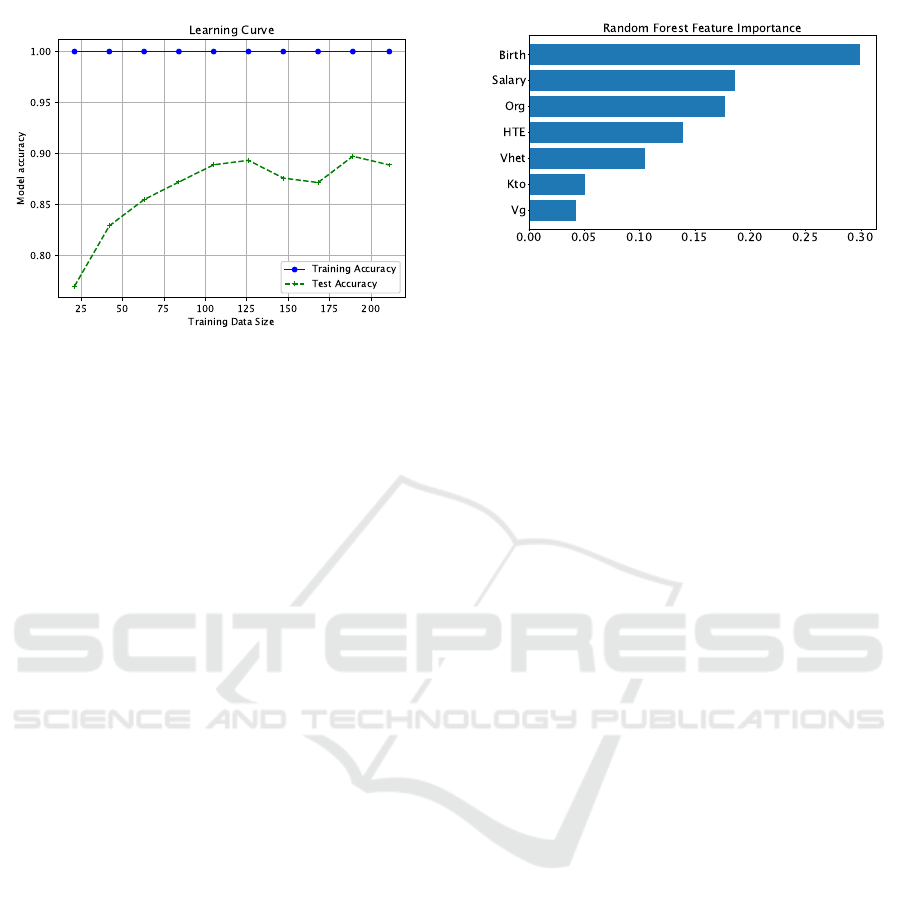
Figure 1: Performance of Random Forest Classiﬁer in terms

of accuracy.

1. 100 trees in the forest.

2. The gain impurity measure to divide the split from

the root node and for subsequent splits.

3. 2 samples to split an internal node.

The dataset D is divided into training and test data

– 80% of D is used to train RF and the remaining

20% is used as test data, also referred to as the “hold

out test data”. Let us represent the training data using

train

and the hold out test data using D

test

. The train-

ing progress of RF is illustrated in Fig. 1. The x-axis

represents the number of training datapoints and the

model accuracy is plotted along y-axis. The blue bold

line represents the accuracy of RF within the train-

ing data D

train

. The green dashed line represents the

accuracy of RF on the hold out test data D

test

. We

observed that the training accuracy is very close to

1 after training with just 25 datapoints from D

train

The accuracy on the test data D

test

, however, is low

at the beginning. As RF is trained on more data, the

test accuracy increases to 0.87. Hence, the accuracy

of RF is strictly better than p (= 0.72). Let Y

(X)

represent the map found by RF after training using

train

. It follows from the discussion in Section 3.3

that H



(X)|X



< H(Y ), that there is information

about Y in X , and that the knowledge of X reduces

the uncertainty in Y . RF is able to exploit some “gen-

der pattern” in X in order to predict the gender Y at a

rate that is better than guessing (completely disregard

X when predicting Y ). Put another way, suppose there

is no gender information in X, then the RF predictions

can only be as good as guessing.

Remark 1. The RF worked admirably well for our

purpose – to illustrate our idea. It may not be the

optimal choice for another use-case, involving a dif-

ferent dataset. One workaround involves training an

ensemble of classiﬁers, instead of a single one. We

Figure 2: Feature Ranking.

then compare the accuracy of the ensemble to p for

diagnostics. The accuracy of the ensemble equals the

maximum of the classiﬁer accuracies.

4.3 Feature Importance Analysis

The feature importance score measures the contribu-

tion of a particular feature to the prediction accuracy,

higher scores indicate greater contributions. The top

scoring features are more likely to have more Y in-

formation (gender information), as compared to low

scoring features. As illustrated in Fig. 2, the date of

birth is the highest ranked feature in our experiment.

Out of all the features, it is likely to have the most

gender information. This would be accounted for in

cases such as Karlstad University, where the more ju-

nior individuals in these departments are women. The

second highest ranked feature is salary, and again, this

contains gendered information, given that women in

Karlstad University, as elsewhere, are more likely to

be in more junior positions and have lower salaries.

Having said that, it must be noted that the highest

salary is earned by a female Professor in our database.

However, the corresponding datapoint is treated as an

outlier by the classiﬁcation algorithm.

It must be noted that there are several other stud-

ies that look at gender inequality in Technology, see,

e.g., (Jaccheri, 2022). In particular, (Jaccheri, 2022)

considers the under-representation of women in the

ﬁeld of Computer Science. Best practices are also

presented for attracting, retaining, encouraging, and

inspiring women in the future. The point of de-

parture of our work, as compared to these studies,

is that we present an automated way of detecting

gender-bias, by estimating a suitable conditional en-

tropy using ML. We therefore provide a simple and

automated way of diagnosing possible gender biases

within organizations. If a gender bias is detected by

our framework, then the solutions highlighted in (Jac-

cheri, 2022) can be employed to improve the situa-

tion.

Information Theoretic Deductions Using Machine Learning with an Application in Sociology

327

5 CONCLUSIONS

Given observations of random variables X and Y , we

presented a ML based framework to estimate the con-

ditional entropy H(Y |X). Our framework is applica-

ble for discrete-valued X and bi-valued Y . We trained

a classiﬁcation algorithm A to predict Y , given X . The

training dataset was constructed using the X and Y ob-

servations. Algorithm A yielded Y

, an approxima-

tion of Y. Then, we used the prediction accuracy to

calculate H(Y

(X)|X), an approximation of H(Y |X).

We formally showed that H(Y |X) < H(Y ) when the

prediction accuracy is strictly greater than p, where p

is deﬁned in equation (2). We thus obtained a sim-

ple sufﬁcient condition on the accuracy to check the

bias of the given dataset. We illustrated our method-

ology by analyzing the employee database from Karl-

stad University. We also discussed how ML tools such

as feature importance scores can be used to obtain

deeper insights.

REFERENCES

Beirlant, J., Dudewicz, E. J., Gy

orﬁ, L., Van der Meulen,

E. C., et al. (1997). Nonparametric entropy estima-

tion: An overview. International Journal of Mathe-

matical and Statistical Sciences, 6(1):17–39.

Bishop, C. M. and Nasrabadi, N. M. (2006). Pattern recog-

nition and machine learning, volume 4. Springer.

Darbellay, G. A. and Wuertz, D. (2000). The entropy as a

tool for analysing statistical dependences in ﬁnancial

time series. Physica A: Statistical Mechanics and its

Applications, 287(3-4):429–439.

Dimpﬂ, T. and Peter, F. J. (2013). Using transfer entropy

to measure information ﬂows between ﬁnancial mar-

kets. Studies in Nonlinear Dynamics and Economet-

rics, 17(1):85–102.

Drees, J. P., Gupta, P., H

ullermeier, E., Jager, T., Konze, A.,

Priesterjahn, C., Ramaswamy, A., and Somorovsky, J.

(2021). Automated detection of side channels in cryp-

tographic protocols: Drown the robots! In Proceed-

ings of the 14th ACM Workshop on Artiﬁcial Intelli-

gence and Security, pages 169–180.

Golder, A., Das, D., Danial, J., Ghosh, S., Sen, S., and Ray-

chowdhury, A. (2019). Practical approaches toward

deep-learning-based cross-device power side-channel

attack. IEEE Transactions on Very Large Scale Inte-

gration (VLSI) Systems, 27(12):2720–2733.

Goodfellow, I., Bengio, Y., and Courville, A. (2016). Deep

learning. MIT press.

Gupta, P., Ramaswamy, A., Drees, J. P., H

ullermeier, E.,

Priesterjahn, C., and Jager, T. (2022). Automated in-

formation leakage detection: A new method combin-

ing machine learning and hypothesis testing with an

application to side-channel detection in cryptographic

protocols.

Hastie, T., Tibshirani, R., Friedman, J. H., and Friedman,

J. H. (2009). The elements of statistical learning: data

mining, inference, and prediction, volume 2. Springer.

Heiberger, R. H. (2022). Applying machine learning in so-

ciology: How to predict gender and reveal research

preferences. KZfSS K

olner Zeitschrift f

ur Soziologie

und Sozialpsychologie, pages 1–24.

Jaccheri, L. (2022). Gender issues in computer science re-

search, education, and society. In Proceedings of the

27th ACM Conference on on Innovation and Technol-

ogy in Computer Science Education Vol. 1, pages 4–4.

MacKay, D. J., Mac Kay, D. J., et al. (2003). Information

theory, inference and learning algorithms. Cambridge

university press.

Molina, M. and Garip, F. (2019). Machine learning for so-

ciology. Annual Review of Sociology, 45:27–45.

Pham, D.-T. (2004). Fast algorithms for mutual information

based independent component analysis. IEEE Trans-

actions on Signal Processing, 52(10):2690–2700.

Zajko, M. (2022). Artiﬁcial intelligence, algorithms,

and social inequality: Sociological contributions

to contemporary debates. Sociology Compass,

16(3):e12962.

ICPRAM 2024 - 13th International Conference on Pattern Recognition Applications and Methods

328