Large Filter Low-Level Processing by Edge TPU

Gerald Krell

and Thilo Pionteck

Institute for Information and Communication Technology, Otto von Guericke University Magdeburg,

Universitätsplatz 2, Magdeburg, Germany

Keywords:

Edge TPU, Tensor Flow, Preprocessing, Low-Level Processing, Deep Learning.

Abstract:

Edge TPUs offer high processing power at a low cost and with minimal power consumption. They are partic-

ularly suitable for demanding tasks such as classiﬁcation or segmentation using Deep Learning Frameworks,

acting as a neural coprocessor in host computers and mobile devices. The question arises as to whether this

potential can be utilized beyond the speciﬁc domains for which the frameworks are originally designed. One

example pertains to addressing various error classes by utilizing a trained deconvolution ﬁlter with a large ﬁl-

ter size, requiring computation power that can be efﬁciently accelerated by the powerful matrix multiplication

unit of the TPU. However, the application of the TPU is restricted due to the fact that Edge TPU software is

not fully open source. This limits to integration with existing Deep Learning frameworks and the Edge TPU

compiler. Nonetheless, we demonstrate a method of estimating and utilizing a convolutional ﬁlter of large size

on the TPU for this purpose. The deconvolution process is accomplished by utilizing pre-estimated convolu-

tional ﬁlters ofﬂine to perform low-level preprocessing for various error classes, such as denoising, deblurring,

and distortion removal.

1 INTRODUCTION

In this paper, we introduce the utilization of Edge

Tensor Processing Units (Edge TPUs) for the low-

level processing of video streams. This task typ-

ically demands signiﬁcant computational resources

and is often performed in close proximity to the sen-

sor within the processing pipeline, before any subse-

quent high-level image processing can occur.

Edge computing aims to process and store data in

close proximity to its sources (Merenda et al., 2020;

?). According to (Yazdanbakhsh et al., 2021), Ten-

sor Processing Units (TPUs) were initially developed

to accelerate machine learning inference within data

centers and later extended to support machine learn-

ing training. Edge TPUs have been introduced in a

limited number of products as inference accelerators

at the edge, positioned near sensors or databases.

Typical applications of Edge TPUs, as highlighted

by (Coral, 2021a), include image classiﬁcation, ob-

ject detection, semantic segmentation, pose estima-

tion, and speech recognition.

One signiﬁcant challenge when applying the Edge

TPU to non-standard applications is the limitation of

its function set. This limitation is illustrated in Fig-

ure 1. While TensorFlow encompasses a wide array of

https://orcid.org/0000-0002-5526-0446

features for deep learning training and inference, Ten-

sorFlow Lite (Google, 2021) is designed to optimize

models for less resource-intensive implementations,

such as mobile applications or embedded devices like

the Edge TPU.

TensorFlow Lite offers a subset of the TensorFlow

API speciﬁcally tailored for machine learning on mo-

bile and edge devices. It includes speed-optimized

functions for hardware implementation and quantiza-

tion techniques to represent data and model parame-

ters as integers.

TensorFow

ensorFow

Lite

Edge TPU

MatMul

BatchMatMul

SparseTensorDenseMatMul

Conv2D

DepthwiseConv2D

TransposeConv

Figure 1: TensorFlow API function set and subsets with

function candidates for Large Filter low-level processing

The function set of the Edge TPU is even smaller

which means that non-supported functions are out-

sourced and executed on the hosting CPU. An even

smaller set is supported by the EdgeCompiler (Coral,

2021b)

464

Krell, G. and Pionteck, T.

Large Filter Low-Level Processing by Edge TPU.

DOI: 10.5220/0012370500003660

Paper published under CC license (CC BY-NC-ND 4.0)

In Proceedings of the 19th International Joint Conference on Computer Vision, Imaging and Computer Graphics Theory and Applications (VISIGRAPP 2024) - Volume 3: VISAPP, pages

464-473

ISBN: 978-989-758-679-8; ISSN: 2184-4321

Hence, we illustrate which functions can be em-

ployed for low-level processing using the Edge TPU.

Figure 1 offers a comparison between the extensive

function set of TensorFlow and TensorFlow Lite and

the highly limited set supported by the Edge Com-

piler. We identify potential functions suitable for our

targeted image low-level processing.

Regrettably, some promising func-

tions, such as MatMul, BatchMatMul, or

SparseTensorDenseMatMul for direct matrix opera-

tions, are not available for the Edge TPU. TensorFlow

provides the Conv2d operation, commonly used in

Convolutional Neural Networks (CNNs). However,

the Edge TPU only supports the separable version,

DepthwiseConv2D, which should sufﬁce for most

ﬁltering tasks.

In the realm of image low-level processing, convo-

lution serves as the mathematical foundation for lin-

ear ﬁltering. This entails convolving a one or more-

dimensional image with a corresponding one or more-

dimensional ﬁlter kernel. When working with separa-

ble ﬁlter kernels, separable ﬁltering is performed in

each dimension. This approach helps conserve math-

ematical operations and, as a result, accelerates pro-

cessing speed.

To achieve this, Deep Learning (DL) models are

developed to implement deconvolution ﬁlters. These

models are estimated through a training process that

utilizes original and degraded images, taking into ac-

count even unknown properties of the image acquisi-

tion system.

Our research demonstrates that these deconvolu-

tion models can be effectively implemented as ﬁ-

nite impulse response (FIR) ﬁlters on Edge TPU

hardware, as provided by the Coral USB accelerator

(Coral, 2022).

The paper is structured as follows:

First, it begins by presenting the tools employed to

apply the Edge TPU for preprocessing video streams.

This is followed by an exploration of the processing

power available in the matrix multiplication unit of

the Edge TPU, in comparison to the requirements of

the targeted preprocessing model.

Next, the paper delves into the mathematical for-

mulation of convolution to model the image degrada-

tion process. It introduces the deconvolution model,

which is utilized to estimate the restoration param-

eters necessary for low-level processing. The paper

also elucidates how model parameters for restoration

can be derived from undistorted and distorted exam-

ple images.

The ﬁnal section of the paper showcases experi-

ments related to model estimation and its execution

on the Edge TPU using sample data. Additionally, it

evaluates the results of the restoration process in re-

lation to model parameters. The paper also demon-

strates the advantages of using large ﬁlter sizes in dif-

ferent aspects.

2 RELATED WORK

The stages of low-level processing, such as ﬁltering

and noise suppression, although not explicitly men-

tioned, are of paramount signiﬁcance in the context of

most video stream analysis applications. To address

this, (Basler, 2021a) has incorporated an image signal

processor into the digital camera video pipeline for

low-level processing. This processor can be imple-

mented either as a customized chip directly behind the

camera sensor or as an additional component within a

processor (Basler, 2021b), specially designed for ma-

chine learning and computer vision tasks.

In their work, (Sun and Kist, 2022) provides a

comprehensive overview of the properties and appli-

cation areas of Edge TPUs while also discussing their

general limitations.

Additionally, (Abeykoon et al., 2019) successfully

ported networks for image restoration to the Edge

TPU, showcasing its versatility.

Moreover, (Zeiler et al., 2010) introduces Decon-

volutional Networks, a valuable approach for unsu-

pervised construction of hierarchical image represen-

tations, which ﬁnd applications in low-level tasks like

denoising and feature extraction for object recogni-

tion.

Furthermore, research, such as that presented in

(Lecun et al., 1998), demonstrates that hand-crafted

feature extraction can be advantageously replaced by

carefully designed learning machines that can operate

directly on pixel images, as exempliﬁed in character

recognition within the scope of (Lecun et al., 1998).

In their study, (Markovtsev, 2019) delve into the

interaction between TensorFlow and the Edge TPU.

They discuss the availability of convolutional oper-

ations and fully connected neural inference opera-

tions on the Edge TPU, taking advantage of the robust

arithmetic hardware of the TPU. Furthermore, they

demonstrate how motion blur can be simulated using

the Edge TPU with DepthwiseConv2d.

In a different research effort, (Yazdanbakhsh et al.,

2021) reported on the inference of 234K distinct con-

volutional neural networks applied to three different

categories of Edge TPU accelerators. The research

involved measuring latency under varying calculation

graph depth and width, and it revealed high inference

accuracy.

Large Filter Low-Level Processing by Edge TPU

465

Additionally, (Civit-Masot et al., 2021) compares

the application of Edge TPUs to eye fundus image

segmentation with a Single Board Computer lacking

deep learning acceleration. The study demonstrates

that machine learning-accelerated segmentation can

achieve processing times below 25 ms per image, un-

derscoring the efﬁciency of Edge TPU-based solu-

tions.

3 TOOLS

3.1 Workﬂow

While the TPU’s CISC instruction set consists of only

a limited number of instructions (Harald Bögeholz,

2017), direct programming of the Edge TPU (ETPU)

is not feasible due to the fact that the available ETPU

compiler and its controlling shared library are propri-

etary (Markovtsev, 2019). Consequently, ETPU pro-

gramming typically relies on utilizing existing Ten-

sorFlow Lite models in conjunction with the ETPU

compiler.

Instead of directly programming the ETPU, the

standard practice involves compiling established Ten-

sorFlow Lite models using the Edge TPU compiler

to enable their execution on the device. Notably, ex-

isting TensorFlow models need to be converted into

the TensorFlow Lite format, which is constrained by

quantization to unsigned byte integers. It’s worth not-

ing that direct matrix multiplication is not supported

by the Edge TPU, despite the presence of a matrix

multiplication unit in the Edge TPU hardware, which

might suggest suitability for matrix operations.

The workﬂow for converting a TensorFlow model

for the Edge TPU is the following:

1. Model generation by TensorFlow (computation

graph)

2. Convertion to TF Lite format (ﬂatbuffers, quanti-

zation uint8)

3. Invokation of edgetpu_compiler

4. Edge TPU ops delegate, invoking the new model

via the interpreter

In our experiments, we employed Matlab on a PC

to estimate the ﬁnite impulse response (FIR) ﬁlter co-

efﬁcients for deconvolution using sample images, as

described in the experiments section. Subsequently,

these restoration coefﬁcients were used in the Python

framework on a Linux PC with the Edge TPU as an

accelerator to create and compile corresponding Ten-

sorFlow Lite (TF Lite) models for execution on the

Edge TPU.

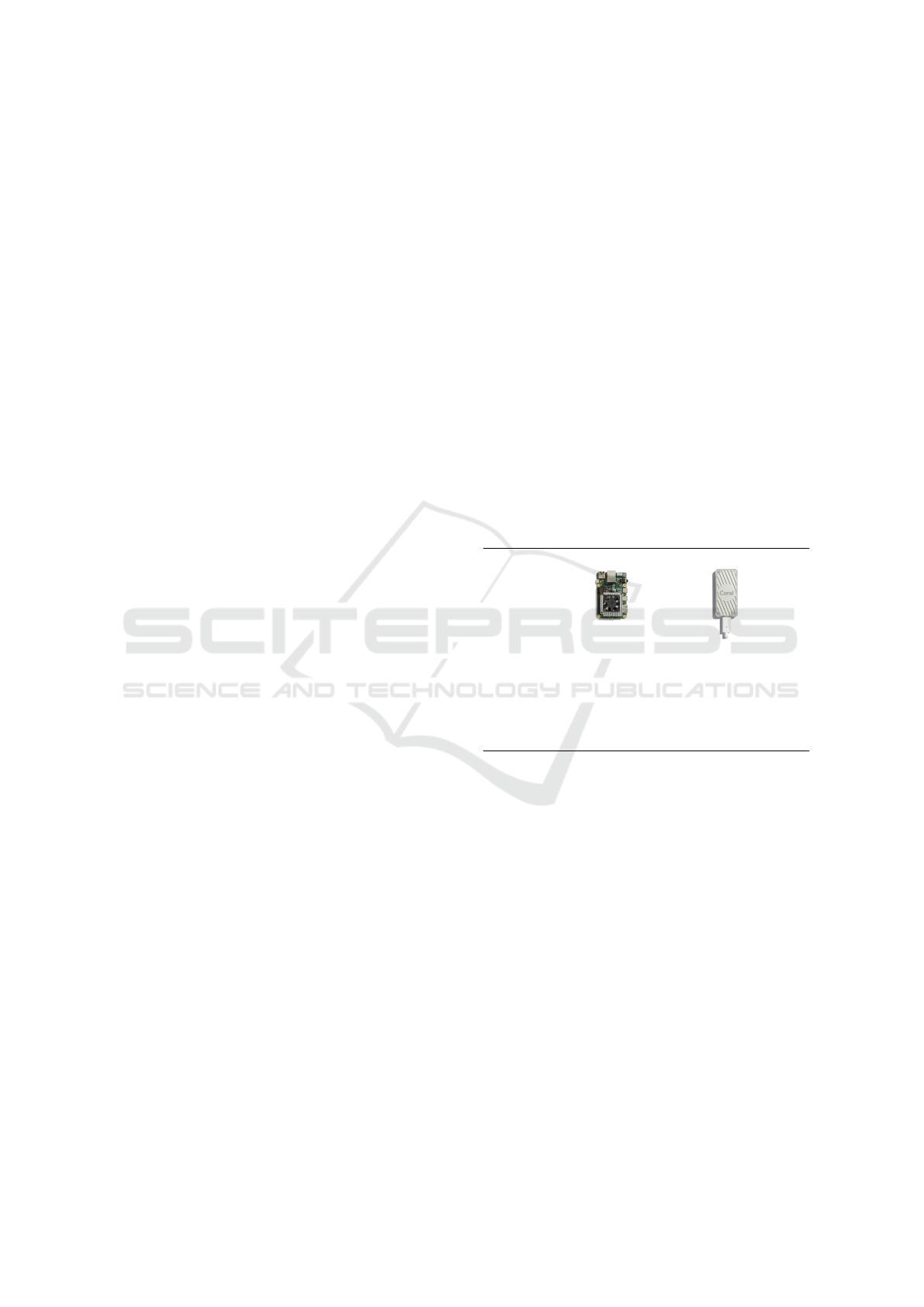
3.2 Hardware

Both the Coral DevBoard and the USB accelerator in-

corporate the same Edge TPU and have been com-

pared, as shown in Figure 2. The former is capable of

direct integration with a camera sensor and operates

independently with its own Linux module.

The latter, on the other hand, can function as a co-

processor for a Linux PC or a Raspberry PI. Video

streams can be transmitted via a network connection.

When it comes to developing models, working with

the USB accelerator is somewhat more convenient.

This is because models can be compiled directly by

the host and then transferred to the coprocessor.

In contrast, the DevBoard’s operating system is

quite limited and not ideal for model estimation or

compilation for the Edge TPU. These tasks must be

performed on a separate host computer, and the com-

puted models must be subsequently transferred to the

DevBoard in an additional step.

DevBoard

USB accelera-

tor

advantages

integrated pe-

ripherals, direct

sensor connec-

tion (camera on

board), no load

on host

direct connec-

tion to host

(e.g. PC or

Raspberry PI)

disadvantages

no compilation

of models, lim-

ited functions

of mendel linux

no integrated

peripherals

Figure 2: Comparison between USB accelerator and

DevBoard.

4 PERFORMANCE

CONSIDERATIONS

In (Harald Bögeholz, 2017), it is noted that Ten-

sor Processing Units (TPUs) have a theoretical up-

per limit of 92 T (tera) operations per second. This

high processing capacity opens the door to intriguing

applications that require real-time processing of large

data streams.

On the other hand, the Edge TPU is designed for

mobile devices to run TensorFlow Lite models and

provides a maximum processing power of 4 T op-

VISAPP 2024 - 19th International Conference on Computer Vision Theory and Applications

466

erations per second (Wikipedia contributors, 2021).

While this is signiﬁcantly less powerful compared to

TPUs, it is still a substantial amount of processing

power, primarily dedicated to model inference tasks.

The proposed low-level processing, based on de-

convolution, aims to be implemented through deep

learning (DL) models that realize ﬁnite impulse re-

sponse (FIR) ﬁlters on the Edge TPU. Given the Edge

TPU’s robust arithmetic hardware, a critical question

arises regarding the size of FIR ﬁlters that can be ef-

fectively implemented.

Let M

ETPU

denote the processing power of one

Edge TPU clock cycle, representing the number of

multiplications-accumulations (MACs) that the Edge

TPU can compute per clock cycle. Assuming a rela-

tionship R between the Edge TPU clock and the pixel

clock, the maximum available processing power of

the Edge TPU for real-time processing of one pixel

is deﬁned as:

max

= M

ETPU

· R . (1)

Depending on the speciﬁc Edge TPU model and the

resolution of the video stream, the value of R may

typically fall within the range of 10. We can now

compare this provided processing power M

max

for one

pixel with the required processing power M

req

for ﬁl-

tering one pixel, both in the case of non-separable and

separable ﬁltering.

4.1 Non-Separable Filter

Given a ﬁlter size of F

in two dimensions for a non-

separable ﬁlter, and considering C color channels, the

required computational costs for processing one pixel

are deﬁned as:

req

= F

·C

. (2)

The assumption of two dimensions is motivated by

the Edge TPU’s primary focus on processing 2-D im-

age streams. It is also assumed that the horizontal

and vertical ﬁlter sizes are equal, which is often the

case for many tasks and is sufﬁcient for a rough es-

timation. The square of channel numbers accounts

for cross-couplings between the channels, which con-

sider mutual inﬂuences between the channels. Such

ﬁlters can handle color errors at edges and even facil-

itate color space rotation when needed.

We ﬁnd the maximum ﬁltersize F

max

by rearrang-

ing equation 2 according to F

and substituting M

req

by M

max

and get

max

ETPU

· R

(3)

Given that M

ETPU

= 4Ki for an Edge TPU matrix mul-

tiplication unit with a size of 4096, and assuming that

the Edge TPU clock is 10 times faster than the pixel

clock (R = 10), we can calculate the maximum ﬁlter

size F

max

as follows: F

max

4Ki·10

= 67.

If we don’t need to consider cross-coupling be-

tween color channels in the ﬁltering process and can

treat the color channels independently, the processing

costs speciﬁed in (2) can be reduced to:

req−wo

= F

·C (4)

This represents the required MACs per pixel with-

out cross-coupling, providing the processing power

needed when there’s no coupling between color chan-

nels.

For a ﬁlter without cross-coupling, the maximum

ﬁlter size approximately doubles:

max−wo

ETPU

· R

4Ki · 10

= 116 .

(5)

Indeed, ﬁlter sizes of this magnitude are quite com-

fortable and versatile. They are not only suitable

for tasks like noise cancellation and deblurring but

can also handle geometric transformations to com-

pensate for lens distortions or perform other coordi-

nate manipulations effectively. This level of process-

ing power opens up a wide range of applications in

image enhancement and correction, making it a valu-

able capability for the Edge TPU.

4.2 Separable Realization

For separable ﬁlters, the situation further improves as

the calculation costs reduce proportionally from F

. This results in the maximum possible separable

ﬁlter size given by:

max−sep

ETPU

· R

4Ki · 10

2 · 3

= 2275 (6)

This allows for signiﬁcantly larger separable ﬁlter

sizes when considering cross-couplings, and even

about three times larger ﬁlter sizes for ﬁlters without

cross-coupling.

With the substantial ﬁlter sizes achievable, en-

abling full coupling over the entire image size by

the ﬁlter becomes realistic for typical image resolu-

tions. If these ﬁlters are available as space-variant

ﬁlters, they could be effectively employed for vari-

ous error correction tasks, including compensation of

distortions that are addressed through warping. This

level of processing capacity would offer sufﬁcient re-

sources for what can be considered as "convenient

warping" in combination with ﬁltering, providing a

versatile and powerful solution for a range of image

processing and correction needs.

Large Filter Low-Level Processing by Edge TPU

467

On the other hand, it’s important to note that sepa-

rable ﬁltering is not well-suited for certain tasks, such

as the removal of rotational blur or certain types of

distortions. Separable ﬁlters are most effective for

ﬁlters with simple spatial dependencies in the hori-

zontal and vertical directions. For ﬁlters with com-

plex, non-axial dependencies between pixels, separa-

ble ﬁlters may not be as suitable, and other methods

or more complex ﬁlter designs may be required to ad-

dress these tasks effectively.

5 CONVOLUTION MODEL

The continuous formulation of convolution is repre-

sented by the equation:

g(x) =

∞

−∞

h(ξ) f (x −ξ)dξ = h ∗ f . (7)

Here, the convolution result at a given position, de-

noted as g(x), is obtained through the inﬁnite inte-

gration of the product of functions h and the shifted

function f over the variable ξ.

In digital signal processing, we work with a dis-

crete and limited form of convolution. We represent

the signal f as a vector

⃗

f containing discrete samples,

and the ﬁlter as a vector

⃗

h, resulting in the convolu-

tion operation denoted as ∗. This discrete convolution

yields the result ⃗g in vector representation:

⃗g =

⃗

h ∗

⃗

f (8)

Here, the resulting convolution samples in the vec-

tor ⃗g are obtained through the convolution operation

∗ between the vectors

⃗

h and

⃗

f , where

⃗

h contains the

coefﬁcients of the ﬁlter h and

⃗

f contains the samples

of the signal f .

When performing convolution over a ﬁlter with M

sample points, where the index is denoted as j, the

discrete convolution result is calculated using the fol-

lowing sum for each sample point with index i:

M−1

∑

j=0

i− j

. (9)

This calculation is carried out for N sampling points,

where i varies within the range [0,N − 1]. However,

when choosing the range i = 0, 1, 2,. . ., N − 1, as-

sumptions must be made for negative indexes of f .

One common approach is to use zero padding, which

means that any negative indices of f are assumed to

be zero.

We can represent the convolution as the multipli-

cation of a matrix by a vector, as deﬁned in (10). This

can be expressed as:







N−1













M−1

·· · h

0 ·· · 0

0 h

M−1

·· · h

0 ·· · 0

0 ·· · 0 h

M−1

·· · h

0 ·· · 0 h

M−1

·· · h













−(M−1)

−1

N−1







(10)

or shorter

⃗g = H

⃗

(11)

Here, ⃗g and

⃗

are vectors that contain discrete values

and can be used to represent result and input images,

respectively, in the context of image processing.

To obtain a result vector with N elements, the in-

put vector f must be extended by M − 1 elements

above to form

⃗

f ex since, in the convolution equation

(9), otherwise, the index range of f would fall below

the range of i. Similarly, the matrix H is extended on

the left by M −1 columns to become H

In the ﬁeld of signal processing, various strategies

are discussed for implicit extension at the borders of

limited discrete signals, such as periodic or mirrored

extension. A practical assumption, also applicable for

hardware implementations as a data stream, is to set

these margin values to zero, a technique known as

zero padding. In this case,

⃗

f is extended with zeros

for negative indices.

The convolution matrix H is a sparse and circulant

Toeplitz matrix with a size of N by N + M − 1, where

each row is a right circular shift of the row above it,

and the elements in the main and side diagonals are

equal. However, this characteristic does not hold for

space-variant systems in which the ﬁlter h is depen-

dent on the location x.

When setting the border elements to zero, the ma-

trix equation (10) can be rewritten as follows:







N−1













M−1

··· h

0 h

M−1

··· h













N−1







(12)

⃗g = H

⃗

f . (13)

The matrix H, when border elements are set to zero,

forms a non-circulant square Toeplitz matrix. When

dealing with two or more dimensional signals, as is

common in image processing, the data needs to be

vectorized (Andrews and Hunt, 1977). Although a

general matrix multiplication is not available in the

VISAPP 2024 - 19th International Conference on Computer Vision Theory and Applications

468

supported Edge TPU functions, the speciﬁc case of

multiplying a Toeplitz matrix (ﬁlter) by a vector (for

1D or 2D images) is provided by convolution func-

tions. This enables efﬁcient processing of multidi-

mensional signals and images using the Edge TPU’s

capabilities.







N−1













N−1

·· · f

N−M













M−1







(14)

⃗g =

⃗

f ∗

⃗

h = F

⃗

h (15)

Utilizing convolution to model the process of image

degradation due to imperfections in the optical system

of image acquisition is a common approach in image

processing. Typically, additional noise needs to be

considered, resulting in the convolution equation:

⃗

ˆg =⃗g +⃗n (16)

Deconvolution aims to ﬁnd a compensation for con-

volution using a function represented by a discrete

vector

⃗

h in such a way that it minimizes the differ-

ence between the convolved result

⃗

ˆg ∗

⃗

h and the origi-

nal image

⃗

f . Mathematically, deconvolution seeks to

minimize the following objective:



⃗

ˆg ∗

⃗

h −

⃗



→ min . (17)

Deconvolution, even though it is a linear system, is

often an ill-conditioned problem, which implies that

it may lack a unique or stable solution. To address

this challenge, we investigate approaches to ﬁnding

well-posed solutions for estimating model parameters

in a broader context. These techniques are applied

to achieve reliable and stable deconvolution results,

mitigating the ill-conditioned nature of the problem.

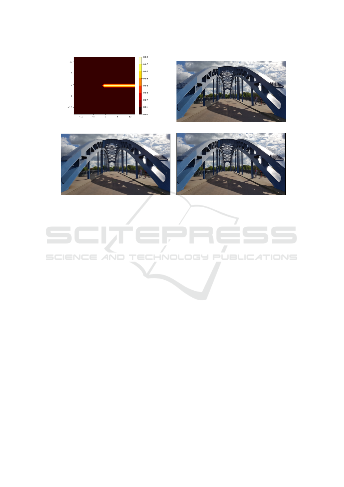
6 EXPERIMENTS

6.1 Training Data Generation

As an example, the motion blur ﬁlter of (Markovtsev,

2019) was used to generate a degraded version of a

test image (see Figure 3)

For 2-dimensional image ﬁltering, both the image

and the ﬁlter need to be vectorized to be used in the

matrix equation. If we consider

⃗

as the vectorized

original image and

⃗

as the blurring vector obtained

by vectorizing the ﬁlter kernel, we can represent the

motion-blurred image in vectorized form as:

⃗

∗

⃗

(18)

This notation is similar to (13), which also deals with

vectorized image and ﬁlter data, assuming that the

boundary elements are set to zero. In this speciﬁc ex-

ample, the ﬁlter kernel, as shown in Figure 3a, de-

ﬁnes

⃗

. The kernel size is 21 by 21, resulting in

N = 21 · 21 = 441 MAC operations per pixel. To

simulate a motion blur of approximately 10 pixels in

the horizontal direction, most elements of

⃗

h are set

to zero, except for the values located on a horizontal

line in the vertical middle of the right half. Convolu-

tion of the input ⃗g, provided by the image from Figure

3b, yields a simulated motion-blur result ⃗g as shown

in Figure 3c.

6.2 Estimation of Model Parameters

For deconvolution, the goal is to ﬁnd a deconvolution

ﬁlter vector

⃗

of length F

to reconstruct a restored

vector, denoted as

⃗

f =

⃗

∗

⃗

(19)

using the motion-blurred image vector

⃗

. The objec-

tive is to make

⃗

f deviate as little as possible from the

original image

⃗

f , and the error signal is represented

by the error vector:

⃗e =

⃗

−

⃗

f (20)

The objective is to minimize the power of this error

signal, making the error as small as possible. This

process aims to reverse the blurring, noise, and other

degradations to restore the image as faithfully as pos-

sible. The goal is to achieve a high-quality restoration

of the original image.

In practice, we aim to minimize the mean squared

deviation between the original and the restoration,

where

indicates the norm:

∥

⃗e

∥



⃗

−⃗g

∗

⃗



→ min . (21)

Expressed as a matrix equation, we have:



⃗

−

⃗



→ min . (22)

The restoration ﬁlter vector,

⃗

, can be estimated by

solving a linear equation system with F

unknowns

in the least mean square sense. This is achieved by

converting equation (19) into a matrix form:

Large Filter Low-Level Processing by Edge TPU

469

(a) (b)

Figure 3: Two-dimensional image data for motion blur generation: 3a Kernel: squared ﬁlter kernel for motion blur simulation

producing blurring ﬁlter vector

⃗

; 3b Input of convolution: original image producing

⃗

; 3c Output of convolution: motion

blur simultation producing

⃗

; 3d Deconvolution Result

O for F

= 27;







−1

N−1













−1

·· · g

N−1

·· · g

N−F













−1







(23)

⃗

∗

⃗

, (24)

where

is the equalization matrix of size n

= N −

+ 1 rows by F

columns assuming that we generate

sample data from all all the elements of

⃗

. The rows

of this matrix consist of pixel-wise shifted sections of

⃗g

. In this case, there can only be a solution for

⃗

the least mean square sense because we assume n

≫

, meaning that we have many more equations than

unknowns. To solve equation (21), we ﬁrst multiply

equation (24) by the transpose (T ) of

from the left:





⃗





⃗

(25)

(26)

We can solve for the restoring ﬁlter as follows:

⃗

. (27)

Here,

represents the pseudo-inverse of

. As-

suming that

has at least F

linearly independent

rows, we can estimate the restoration using equation

(19), resulting in a restored image

⃗

f =

⃗

−⃗e . (28)

that deviates from the original by the error vector ⃗e.

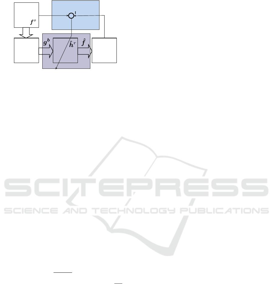
6.3 Running the Inference on the Edge

TPU

In the context of Deep Learning,

⃗

f can be viewed as

the result of inferring the model

⃗

using the input

vector

⃗

, as illustrated in Figure 4. Model estima-

tion is carried out on the host computer using samples

from both the ideal and restored image streams. Infer-

ence is then performed on the Edge TPU to compen-

sate for the errors resulting from image degradation.

This approach estimates the restoring ﬁlter in a

manner similar to an inverse ﬁlter. However, because

equation (22) usually has many more rows than un-

knowns, a solution in the least mean square sense can

be found. This approach takes typical image noise

into consideration, resulting in a more stable and ro-

bust result compared to directly inverting a degrading

ﬁlter matrix H.

VISAPP 2024 - 19th International Conference on Computer Vision Theory and Applications

470

CNN

restored

image

stream

ideal

image

degraded

image

stream

degradation

on host

on ETPU

inference

model estimation

Figure 4: Dimensioning the CNN model for removal of im-

age errors

Based on the training data (see section 6.1) mod-

els of different ﬁlter sizes F

have been estimated by

(27) using Matlab for compensating the motion blur.

Figure 3d show one of the results for F

= 27. In the

practical implementation of the model estimation, not

the complete image is maybe necessary in (27) and

subimages of the whole image can be used. This can

also reﬂect specially varying behaviour.

The estimated Filter models ﬁrst converted into a

quantized TFLite representation and then compiled

for the Edge TPU according to (Markovtsev, 2019).

The inference has then be done on the USB accelera-

tor with the training input image Figure 3c. The result

corresponds to the expected inference result of Figure

3d with little deviations caused by quantization of the

model parameters, but below a visual threshold.

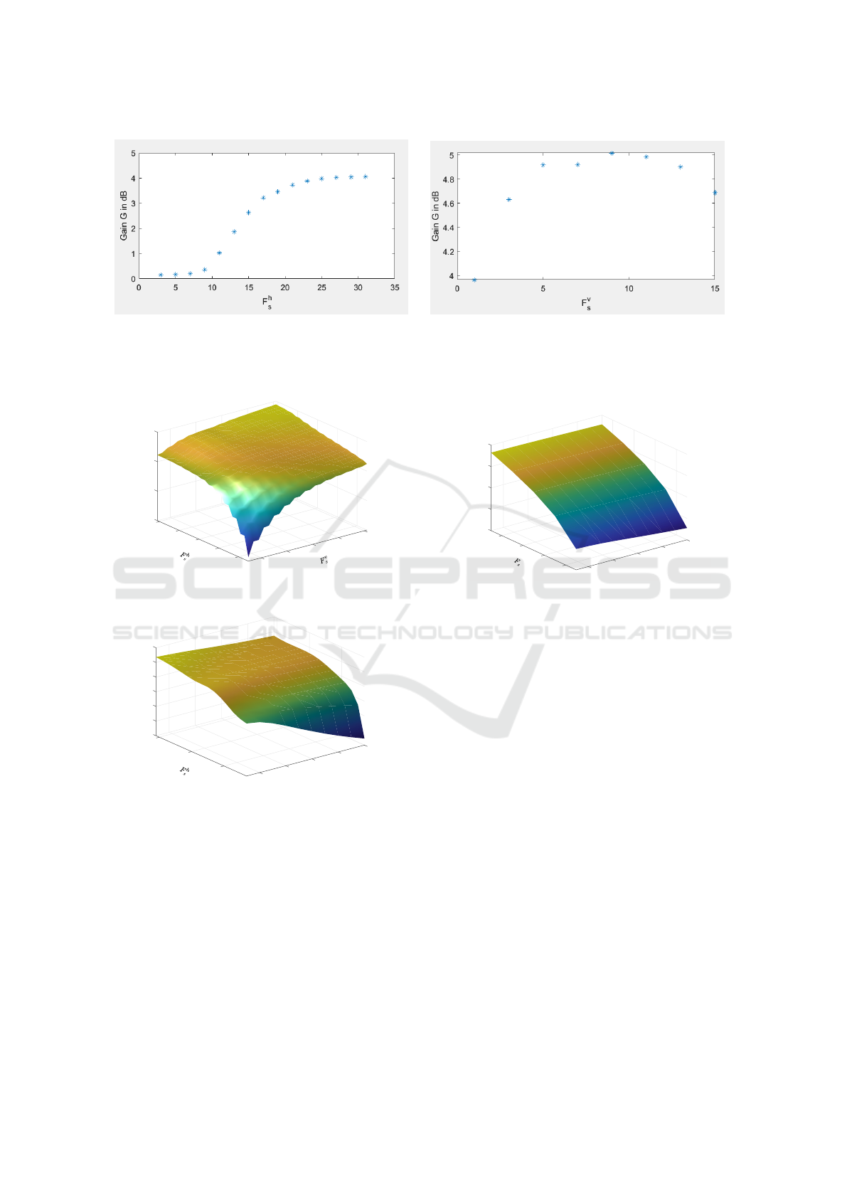
6.4 Inﬂuence of Filter Size

In order to investigate the impact of ﬁlter size onto the

the obtained enhancement we investigated the gain of

PSNR (Peak Signal to Noise Ratio) by applying the

deconvolution ﬁlter model for restoration:

G = PSNR

− PSNR

(29)

where PSNR

= 20

max

∥

⃗

−⃗g

∥

dB is the PSNR of the

input of the deconvolution and PSNR

= 20

max

∥

⃗e

∥

the PSNR of the restoration with I

max

= 255 the max-

imum pixel value.

First we applied deconvolution to the motion

blurred image ⃗g

and changed the horizontal F

in a

range [1,15].

Figure 5 shows the dependency of G on the ﬁlter

size F

. It is obvious that a minimum ﬁlter size of

about F

= 10 is required in order to obtain a mean-

ingful improvement. Above ﬁlter size 30 the growth

of the gain is decreasing rapidly. This behavior can

be explained by the original motion blur of about 7

pixels which should be in the same range as F

Secondly we additionally superimposed normal

distributed noise of 40 dB. We kept the horizontal

ﬁltersize at 27 which could be considered as an op-

timal ﬁlter size for motion blur compensation in hor-

izontal direction and increased the vertical ﬁlter size

steps for F

= 1, 3,· ·· ,15. It is visible that in the cur-

rent situation of noise and blur a ﬁlter size of about

7 is sufﬁcient in order to compensate additionally for

the noise degradation. Together with horizontal ﬁlter

size we come to a total 2 dimensional ﬁlter size of

= F

= 7 ·27 = 189 which is pretty much calcu-

lation per pixel. The separable implementation needs

only F

= F

+ F

= 7 + 27 = 34 which is much re-

duction.

In the next experiment, we show the option to han-

dle different degradation types by application large

ﬁlter sizes in different situations. In Figure 6, we sim-

ulated motion blur of 25 pixels in a direction of 30

degrees and estimated the gain of quality for different

horizontal and vertical ﬁlter sizes.

It becomes obvious that ﬁlter sizes in the range of

blur are required to obtain good performance of the

restoration. Due to the angle of motion the horizon-

tal component is larger than the vertical component.

Correspondingly the the saturation of gain value is

reached quicker.

In 7, we additionally superimposed normally dis-

tributed noise on a motion blurred image by 25 pixels

in horizontal direction and estimated the quality gain

for different horizontal ﬁlters of size F

. The graph

shows that small ﬁlter sizes lead to weak gain, espe-

cially for higher noise levels.

In 8, we additionally superimposed normally dis-

tributed noise on the same motion blurred image and

estimated the quality gain for different 2-dimensional

ﬁlters of same horizontal and vertical sizes. The graph

shows that small ﬁlter sizes lead to weak gain, espe-

cially for higher noise levels.

All the above experiments can be performed in

real-time on the Edge TPU for typical video streams

because the ﬁlter sizes are below of the estimated lim-

its calculated in section 4.1 which is in the range of

one hundered.

7 CONCLUSIONS

We showed how a Deep Learning model for a decon-

volution ﬁlter can be dimensioned from a known input

output relation of an image capturing system and how

it can be inferred on an Edge TPU. The ﬁlter has been

estimated without using knowledge of degrading ﬁl-

ter but on the basis of known original and degraded

image. This implicitly considers the noise impact and

Large Filter Low-Level Processing by Edge TPU

471

(a) (b)

Figure 5: Dependency of quality gain G on ﬁlter sizes F

and F

for the inference example: 5a dependency of Gain on

horizontal ﬁlter size F

for motion blurred image ⃗g

; 5b dependency of Gain on vertical ﬁlter size F

with additional noise

superposition by PSNR = 40dB.

G/dB

Figure 6: Gain G for different horizontal and vertical ﬁlter

sizes with a motion blur of 25 pixels in direction 30 degrees.

N/%

G/dB

Figure 7: Gain G for horizontal motion and different hori-

zontal ﬁlter sizes F

and noise levels.

avoids the otherwise necessity of inverting the degrad-

ing systems.

The Edge TPU allows very long ﬁlter sizes to

be calculated in real-time for low-level processing of

video streams. As part of the digittal camera pipeline

it can act as an electronic lens when the large ﬁlter

is not only used for noise reduction and deblurring

but also for the removal of larger motion blur or geo-

metric lens distortions. We showed promising results

for non-separable ﬁlter sizes in the range of up to one

hundred. With the potentially possible separable ﬁl-

ter size of about two thousand interesting applications

N/%

G/dB

Figure 8: Gain G for different horizontal ﬁlter sizes F

= F

and noise levels.

could be possible which is part for future work.

The Tensor Flow provided function

TransposeConv also has potentially interesting

applications for image error compensation that are

worth exploring in further work. Unfortunately,

the potentially large ﬁlter sizes due to the large

computational power cannot be implemented in a

location-variant manner, severely limiting its appli-

cability. For such applications, tailored hardware

solutions therefore still seem to be the means of

choice.

REFERENCES

Abeykoon, V., Liu, Z., Kettimuthu, R., Fox, G., and Foster,

I. (2019). Scientiﬁc Image Restoration Anywhere. In

2019 IEEE/ACM 1st Annual Workshop on Large-scale

Experiment-in-the-Loop Computing (XLOOP), pages

8–13, Denver, CO, USA. IEEE.

Andrews, H. C. and Hunt, B. R. (1977). Digital image

restoration. Prentice-Hall signal processing series.

Prentice-Hall, Englewood Cliffs, N.J.

Basler (2021a). Design an Eye-Catching Vision System for

Machine Learning with the i.MX 8M Plus Applica-

VISAPP 2024 - 19th International Conference on Computer Vision Theory and Applications

472

tions Processor. embedded_vision/nxp-2021-1/NXP

-TECH-SESSION-EYE-CATCHING-VISION-SYS

TEM-MLAI.pdf.

Basler (2021b). The NXP i.MX 8M Plus Applications Pro-

cessor: Bringing High-Performance Machine Learn-

ing to the Edge. embedded_vision/nxp-2021-2/AI-T

O-THE-EDGE-WP-1-1.pdf.

Civit-Masot, J., Luna-Perejón, F., Corral, J. M. R.,

Domínguez-Morales, M., Morgado-Estévez, A., and

Civit, A. (2021). A study on the use of Edge TPUs for

eye fundus image segmentation. Engineering Appli-

cations of Artiﬁcial Intelligence, 104:104384.

Coral (2021a). Models.

Coral (2021b). TensorFlow models on the Edge TPU. TP

U_Preprocessing/coral_tensorﬂow_nodate1/models-i

ntro.html.

Coral (2022). USB Accelerator.

https://coral.ai/products/accelerator.

Google (2021). TensorFlow Lite | ML for Mobile and Edge

Devices.

Harald Bögeholz (2017). Künstliche Intelligenz: Architek-

tur und Performance von Googles KI-Chip TPU. TP

U_Preprocessing/online_kunstliche_nodate_heise2/

Kuenstliche-Intelligenz-Architektur-und-Performan

ce-von-Googles-KI-Chip-TPU-3676312.html.

Lecun, Y., Bottou, L., Bengio, Y., and Haffner, P. (1998).

Gradient-based learning applied to document recog-

nition. Proceedings of the IEEE, 86(11):2278–2324.

TPU_Preprocessing/LeCun1998GradientbasedLA/C

onvolution_nets.pdf.

Markovtsev, V. (2019). Hacking Google Coral Edge TPU:

motion blur and Lanczos resize.

Merenda, M., Porcaro, C., and Iero, D. (2020). Edge

Machine Learning for AI-Enabled IoT Devices: A

Review. Sensors (Basel, Switzerland), 20(9):2533.

tpu-paper/merenda_edge_2020/Merendaetal.-2020-E

dgeMachineLearningforAI-EnabledIoTDevices.pdf.

Sun, Y. and Kist, A. M. (2022). Deep Learning on Edge

TPUs. arXiv:2108.13732 [cs].

Wikipedia contributors (2021). Tensor processing unit —

Wikipedia, the free encyclopedia. https://en.wikiped

ia.org/w/index.php?title=Tensor_Processing_Unit&

oldid=1056864312. [Online; accessed 20-January-

2022].

Yazdanbakhsh, A., Seshadri, K., Akin, B., Laudon, J.,

and Narayanaswami, R. (2021). An Evaluation of

Edge TPU Accelerators for Convolutional Neural Net-

works. arXiv:2102.10423 [cs]. arXiv: 2102.10423

tpu/yazdanbakhsh_evaluation_2021/2102.10423.pdf.

Zeiler, M., Krishnan, D., Taylor, G., and Fergus, R. (2010).

Deconvolutional networks. In Proceedings of the

IEEE Computer Society Conference on Computer Vi-

sion and Pattern Recognition, pages 2528–2535. TP

U_Preprocessing/Zeiler-2010-1/deconvolutionalnetw

orks.pdf.

Large Filter Low-Level Processing by Edge TPU

473