CaRaCTO: Robust Camera-Radar Extrinsic Calibration with Triple

Constraint Optimization

Mahdi Chamseddine

1,2 a

, Jason Rambach

1 b

and Didier Stricker

1,2 c

German Research Center for Artiﬁcial Intelligence (DFKI), Kaiserslautern, Germany

RPTU Kaiserslautern, Kaiserslautern, Germany

{ﬁrstname.lastname}@dfki.de

Keywords:

Calibration, Camera, Radar, Robotics.

Abstract:

The use of cameras and radar sensors is well established in various automation and surveillance tasks. The

multimodal nature of the data captured by those two sensors allows for a myriad of applications where one

covers for the shortcomings of the other. While cameras can capture high resolution color data, radar can

capture the depth and velocity of targets. Calibration is a necessary step before applying fusion algorithms

to the data. In this work, a robust extrinsic calibration algorithm is developed for camera-radar setups. The

standard geometric constraints used in calibration are extended with elevation constraints to improve the opti-

mization. Furthermore, the method does not rely on any external measurements beyond the camera and radar

data, and does not require complex targets unlike existing work. The calibration is done in 3D thus allowing

for the estimation of the elevation information that is lost when using 2D radar. The results are evaluated

against a sub-millimeter ground truth system and show superior results to existing more complex algorithms.

https://github.com/mahdichamseddine/CaRaCTO.

1 INTRODUCTION

Environment sensing is an integral task in many mod-

ern applications. Whether it is for robotics, surveil-

lance (Roy et al., 2009; Roy et al., 2011), autonomous

or assistive driving (Cho et al., 2014; Chavez-Garcia

and Aycard, 2015), sensors such as camera, radar, and

lidar are used to detect and classify objects and obsta-

cles in the respective environments. The sensors used

have different characteristics which make them com-

plementary rather than redundant. Cameras provide

high resolution color, texture, as well as context in-

formation whereas lidar and radar provide depth and

dimensions. While lidar data is of a higher spatial

density than radar data, the latter is more robust to

weather and lighting conditions and can measure ve-

locities.

Data from the different sensors is usually fused to-

gether to get a better understanding of the state of the

environment. Using the fused data, it is possible to

detect the different objects and obstacles using mul-

timodal features like dimensions and position, veloc-

https://orcid.org/0000-0003-4119-457X

https://orcid.org/0000-0001-8122-6789

https://orcid.org/0000-0002-5708-6023

ity and orientation, etc. (Sugimoto et al., 2004; Wang

et al., 2011; Wang et al., 2014; Kim and Jeon, 2014).

The tasks of sensor fusion however are preceded by

a necessary calibration that aligns the data from all

sensors in a common reference frame so that data as-

sociation is done correctly. This makes calibration an

essential step in any data processing problem.

Lidar sensors still suffer from high retail prices,

and as such have not seen as much commercial adop-

tion as cameras and radar sensors that have been

around for a much longer time. And even though high

resolution 3D radar sensors are starting to gain pop-

ularity (Stateczny et al., 2019; Wise et al., 2021), the

2D radar sensors are still the most widely used type of

radar in commercial applications. Therefore, the cali-

bration approach presented in this work is targeting a

2D radar and camera setup due to low price and wide

adoption.

In this work, an extrinsic calibration algorithm for

camera-radar systems is presented. Unlike other ap-

proaches which project the radar data to 2D, in this

approach, the elevation is not disregarded but rather

estimated with the help of the camera to realize 3D

reconstruction of targets. The work also aims to sta-

bilize the optimization problem against bad initializa-

tion and simplify the calibration setup to make it more

534

Chamseddine, M., Rambach, J. and Stricker, D.

CaRaCTO: Robust Camera-Radar Extrinsic Calibration with Triple Constraint Optimization.

DOI: 10.5220/0012369700003654

Paper published under CC license (CC BY-NC-ND 4.0)

In Proceedings of the 13th International Conference on Pattern Recognition Applications and Methods (ICPRAM 2024), pages 534-545

ISBN: 978-989-758-684-2; ISSN: 2184-4313

Calibration Categories

Affine

Transformation

Projective

Transformation

Extrinsic

Calibration

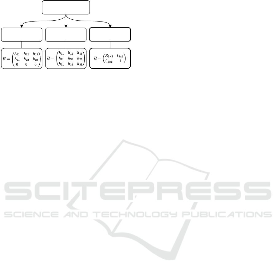
Figure 1: The different calibration categories as presented

by Oh et al. (Oh et al., 2018). Our approach belongs to the

third category.

accessible while maintaining the same quality or im-

proving upon existing algorithms.

The main contributions can be summarized as:

• A camera-radar 3D calibration approach that does

not require external sensing.

• Improved optimization formulation with addi-

tional elevation constraints for improved stability.

• Evaluation against state-of-the-art approaches

using high accuracy optical measurements as

ground truth and showing signiﬁcant improve-

ment.

The rest of the paper is structured as follows: Sec-

tion 2 discusses the related work and previous con-

tributions to the ﬁeld. In Section 3 the problem is

deﬁned, our used notation is explained and the sys-

tem model is described. The proposed method is pre-

sented in Section 4, and then evaluated in Section 5.

Finally, concluding remarks are given in Section 6.

2 RELATED WORK

Several works on camera-radar calibration have been

published. A comparative study by Oh et al. (Oh

et al., 2018) differentiates between three differ-

ent categories of camera-radar calibration (see Fig-

ure 1): afﬁne transformations, projective transforma-

tions, and extrinsic calibration which is the target of

our work.

In the work by Wang et al. (Wang et al., 2011)

and Kim et al. (Kim and Jeon, 2014), an afﬁne trans-

formation is calculated between the 2D radar points

and their corresponding pixel locations in the image.

Pseudo inverse is used to solve a least squares setup of

the two dimensional afﬁne transformation. The qual-

ity of the transformation is measured using the im-

age distance of the transformed radar points relative

to their corresponding image points.

Whereas the 2D afﬁne transformation calibration

estimates six out of nine transformation parameters,

the 2D projective transformation method estimates

the complete 3 × 3 homography between the radar

and camera planes. Sugimoto et al. (Sugimoto et al.,

2004) and then Wang et al. (Wang et al., 2014) use the

projective transformation method for camera-radar

calibration. Even though this method can provide

more accurate results for the calibration than afﬁne

transforms, the calibration disregards the 3D repre-

sentation of the data and only provides point corre-

spondences from the radar plane to the camera plane.

The third calibration category is extrinsic cali-

bration, and the literature shows two different types:

multi-sensor extrinsic calibration combining camera,

lidar, and radar, and camera-radar only extrinsic cali-

bration.

Per

s et al. (Per

c et al., 2019) developed a radar-

lidar-camera calibration method where the 3D lidar

information is used to transform the radar frame in

2D and neglecting the elevation. The optimization is

then performed in the 2D radar plane to estimate a

transformation (rotation and translation) between the

different sensors. Domhof et al. (Domhof et al., 2019)

treat the radar data similarly and euclidean error in 2D

is used for solving the optimization and calculating

the extrinsic parameters. They additionally designed

a complex joint target for camera, lidar, and radar.

Using a 3D radar sensor, Wise et al. (Wise

et al., 2021) develop a continuous extrinsic calibration

method that makes use of the extra dimension mea-

surement as well the radar velocity measurement to

develop a calibration algorithm that does not require

radar retroreﬂectors. While their method properly

takes into consideration the 3D nature of the problem

and the complexity of using specialized targets, it is

limited in application to less widely used 3D radars.

Unlike other camera-radar calibration methods, El

Natour et al. (El Natour et al., 2015a) formulates the

problem with the underlying assumption that the 2D

representations in the image and radar data corre-

spond to targets in 3D, thus the optimization is done

using the 3D form and using the distance between

multiple targets to recover the full 3D representation

from 2D sensors. This allows for 3D reconstruction

of targets after the system is calibrated. However, to

achieve this result, multiple targets need to be present

and the distance between them measured accurately.

The authors try to overcome this limitation in (El Na-

tour et al., 2015b) by moving the sensor system while

keeping the targets ﬁxed and adding the sensor trajec-

tory estimation.

In our work, an extrinsic calibration algorithm is

presented to estimate the rotation and translation be-

CaRaCTO: Robust Camera-Radar Extrinsic Calibration with Triple Constraint Optimization

535

tween the camera and radar sensors and using the 3D

representation of the targets. In contrast to prior work,

only a single retroreﬂector is used without the need

for a complex target design. Furthermore, the algo-

rithm is made stable even with sub-optimal initial-

ization through additional elevation constraints and

the results are veriﬁed against other works using high

quality ground truth system for the ﬁrst time in such

evaluations.

3 PROBLEM DEFINITION

Extrinsic calibration is the task of calculating the

transformation (rotation and translation), between the

coordinate systems of different sensors. The transfor-

mation can then be used to project a point from one

system to the other and also reconstruct the 3D posi-

tion.

For radar calibration, a speciﬁc target is used to

collect and reﬂect the received radar signal. Such tar-

get is called a retroreﬂector characterized by its abil-

ity to reﬂect radiation back at its source (i.e. radar)

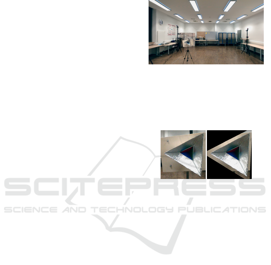
with minimal scattering. In this work, a corner re-

ﬂector is used which has a pyramidal shape made of

3 right isosceles triangles joined at their vertex angle

(see Figures 3 and 4).

3.1 Notation

Since the calibration algorithm estimating the extrin-

sic transformation between two different sensors, it is

ﬁrst necessary to deﬁne the notation used in the rest of

the sections and for this the notation deﬁned in (Ram-

bach et al., 2021) is used.

Let m

= [x

]

⊤

be the point m in a coordi-

nate system A. The rotation and translation to convert

m from system A to system B are then deﬁned as R

and b

respectively such that R

represents the rota-

tion from coordinate system A to B and b

is the origin

of system B represented in system A. The transforma-

tion and its inverse can then be written as

= R

− b

= R

− a

(1)

where R

= R

−1

= R

⊤

and a

= −R

. Thus, m

can be expressed as

= R

+ a

. (2)

Finally, the homogeneous transformation H

from coordinate system A to B can then be expressed



0 1



. (3)

3.2 System Model

The sensor setup is a radar-camera system connected

rigidly and separated by a short baseline much smaller

than the distance to the measured target. To avoid

confusion in the terminology, the coordinate systems

will be referred to as C for camera and S for radar

(sensor). It then follows that R

and R

are the ro-

tations from the radar to the camera system and its

inverse respectively. Similarly, c

is the origin of the

camera in the radar coordinate system s

is the origin

of the radar in the camera coordinate system.

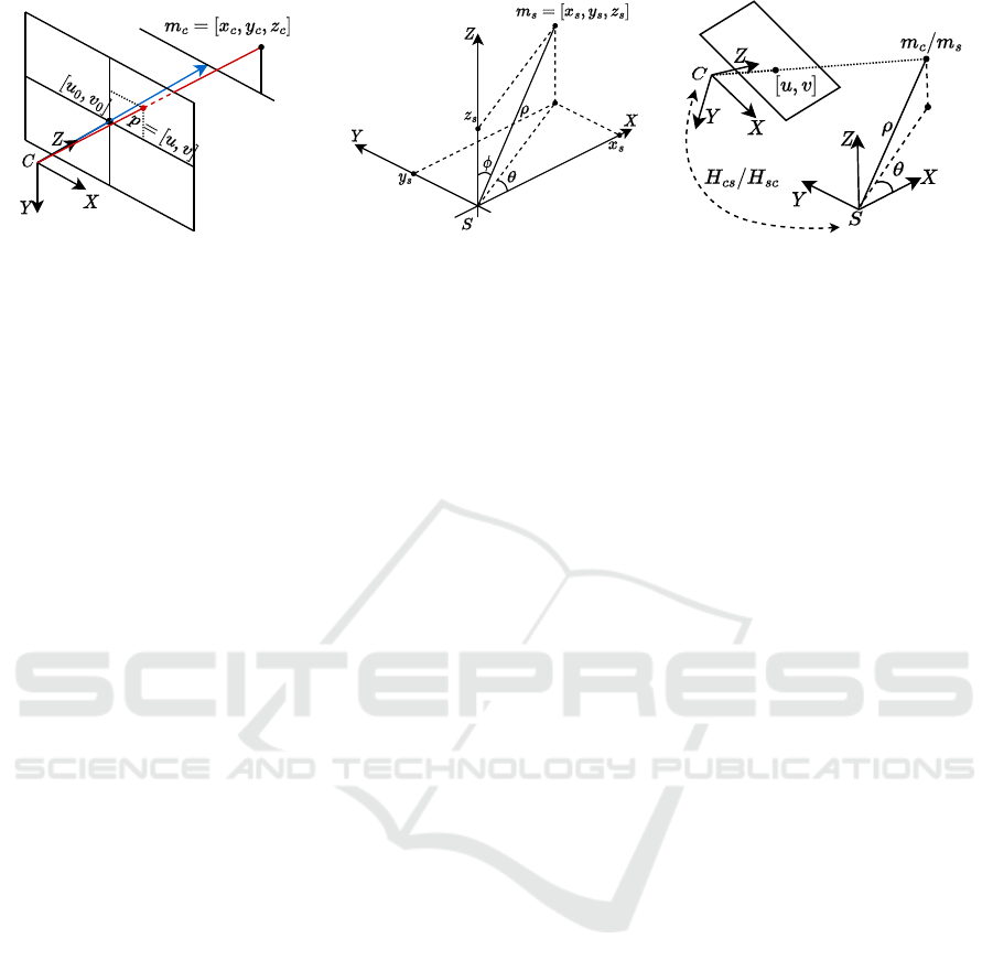
The camera model used is the pinhole model

shown in Figure 2a, and it is used to project a point

= [x

]

⊤

in the camera coordinate system to

p = [u, v, 1]

⊤

on the image plane.

p = Km













0 u

0 f

0 0 1













(4)

where K is the intrinsic parameters matrix of the cam-

era and is be calculated using the standard method

in (Zhang, 2000) and u and v are the pixel coordinates

of the point in an image. The radar is a frequency-

modulated continuous-wave (FMCW) radar that re-

turns the range, azimuth, doppler velocity, as well as

radar cross section (reﬂection amplitude). Only the

range and azimuth (ρ,θ) are used for the calibration.

It can be noticed that the radar does not provide any

elevation information φ, with φ representing the angle

with positive z-axis. The general representation of the

point m

= [x

]

⊤

in the radar coordinate system

is shown in Figure 2b and deﬁned as

= ρ sin φ cos θ,

= ρ sin φ sin θ,

= ρ cos φ,

(5)

since φ is usually unknown, output can only be in-

terpreted in 2D in other approaches (Sugimoto et al.,

2004; Wang et al., 2011; Wang et al., 2014; Kim and

Jeon, 2014; Per

c et al., 2019; Domhof et al., 2019)

and is assumed that φ = π/2.

Overall, a radar point in the radar coordinate sys-

tem can be represented in the camera coordinate sys-

tem using

= R

+ s





= H





(6)

Figure 2c shows the same target represeted in both

camera and radar coordinate systems. Combin-

ing Equation (4) with Equation (6), a relationship de-

ICPRAM 2024 - 13th International Conference on Pattern Recognition Applications and Methods

536

(a) (b) (c)

Figure 2: (a) and (b) show the measurement setup of both the camera and radar respectively. The pinhole model in (a) shows

how an object in 3D can be represented in the camera coordinate system, and the pixel representation on the image plane. The

radar data in (b) is measured in spherical coordinates, the diagram shows how they can be visualized as cartesian coordinates.

(c) shows how an object visible in both the camera and radar frames can be represented in either frames and the transformation

can be used to go from one representation to the other.

scribing a transformation between the radar and im-

age data is then deﬁned as follows

p = [K|0]H





, (7)

where the K matrix is extended by a zero column to

match the dimensions of the H matrix.

4 PROPOSED APPROACH

Our goal is to setup a system of equations to com-

pute the residuals for the optimization. The residuals

are minimized by ﬁnding the parameters of the ex-

trinsic calibration. We ﬁrst deﬁne the geometric rela-

tions that describe the measurements, we then formu-

late the optimization, and ﬁnally we reconstruct the

3D point cloud using the estimated calibration param-

eters.

4.1 Geometric Constraints

Using the measurement principles of the sensors used,

different constraints and relationships can be ob-

served. Given that the distance of a target to the radar

is measured, the locus of the target can be restricted

to a sphere of radius ρ centered at the radar

+ y

+ z

= ρ

. (8)

Knowing the azimuth angle of the target with re-

spect to the radar positive x-axis, target also belongs

to a plane passing through the radar center and per-

pendicular to the xy-plane. The normal vector to the

plane is simply deﬁned at the angle (θ + π/2). Thus

the unit normal vector to the plane passing through

the target point and the radar center is

⃗

n = (cos (θ + π/2),sin (θ + π/2),0)

= (− sin θ, cos θ, 0),

⃗

n = (sin θ, − cos θ, 0).

(9)

The locus of the target in the radar coordinate sys-

tem can then be restricted to the intersection between

the sphere deﬁned in Equation (8) and the plane

sinθ − y

cosθ = 0, x

> 0, (10)

the condition that x

> 0 means that the target should

belong to the positive semi-circle in front of the radar.

The target also belongs to the line passing through

the camera center and (u,v), the target’s projection on

the image plane. This line intersects the semi-circle

from Equations (8) and (10) at one point representing

the position of the target in 3D.

4.2 Optimization Formulation

Based on the constraints deﬁned earlier, an optimiza-

tion system is setup based on Equations (8) and (10)

as follows

+ y

+ z

− ρ

= ε

sinθ − y

cosθ = ε

(11)

where ε

and ε

are the residuals to be minimized as

to ensure the 3D radar points satisfy the constraints.

The position of the target in the image is then used to

derive the representation of m

= [x

]

⊤

in terms

of (u, v) and H

. From Equation (7) the following

can be derived





= H

−1



−1



= H



−1





0 1



−1



(12)

CaRaCTO: Robust Camera-Radar Extrinsic Calibration with Triple Constraint Optimization

537

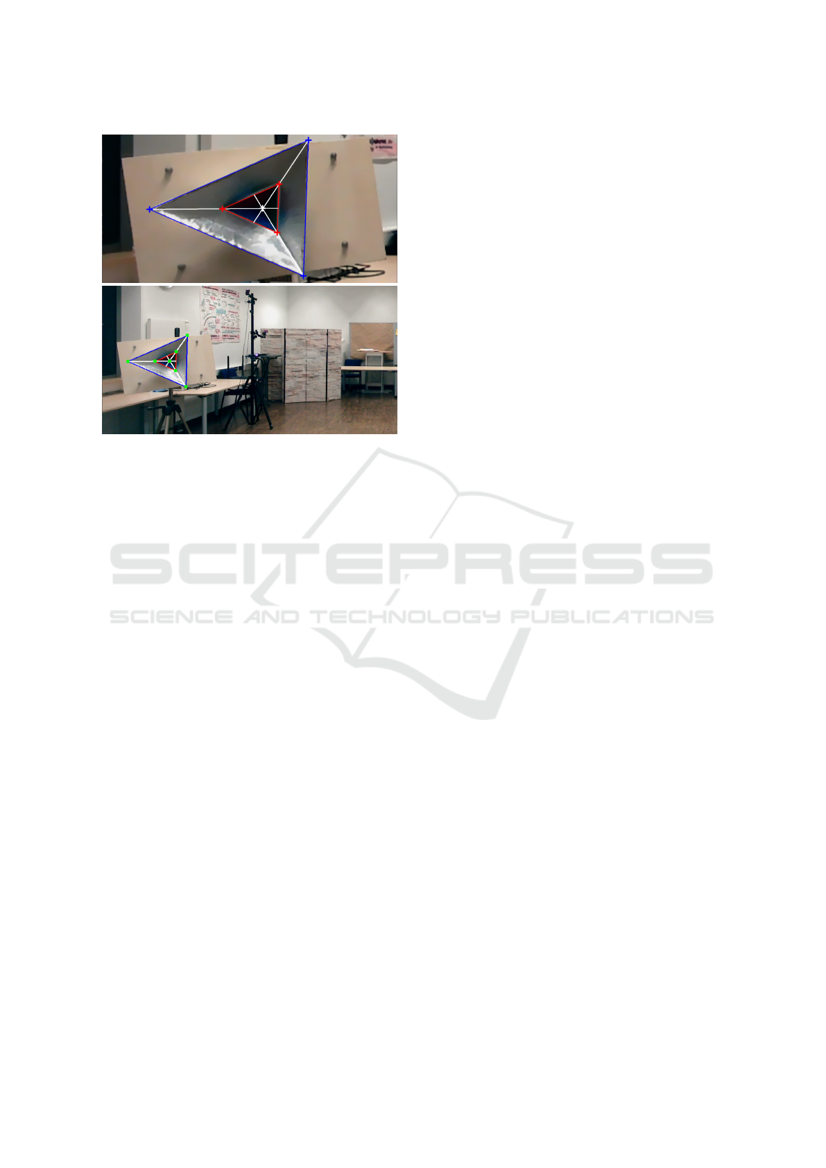
Figure 3: Top: Detection of corners of calibration target, a

minimum of 4 points is needed to solve the PnP problem.

Bottom: the reprojected solution of the PnP problem

(green).

where R

= R

and α, β, and γ are the rota-

tion angles around x, y, and z respectively. So the

parameters to be estimated are the three rotation an-

gles and the three translations represented by c

]

⊤

The last unknown to be estimated in Equation (12)

is z

. Existing work (El Natour et al., 2015a) tack-

les the problem by using a minimum of six ﬁxed tar-

gets and accurate measurement of the distances be-

tween them to estimate z

, whereas (El Natour et al.,

2015b) requires the ability to move the whole radar

camera system to estimate z

as part of the optimiza-

tion. However, in this work we introduce two methods

to estimate z

with a single target measured at differ-

ent positions thus simplifying the setup signiﬁcantly.

4.2.1 Method 1: Using Radar Range as an

Estimate for z

Since z

is a measure of depth of a target with respect

to the camera, and since the radar can directly detect

a target’s depth, it is logical to beneﬁt from the multi-

modal measuring capabilities of the sensor setup and

use z

= ρ. This assumption is limited to the case

when the baseline between the camera and the radar

is much smaller than the measured distance and when

the camera and radar are close to each other.

4.2.2 Method 2: Using Camera

Correspondences to Calculate z

This method overcomes the limitations of the ﬁrst

method and removes the short baseline requirement.

Using the known dimensions of the radar retroreﬂec-

tor and intrinsic calibration matrix K, it is possible to

solve the perspective-n-point (PnP) problem to obtain

the 6 DoF pose in the camera coordinate system (Lep-

etit et al., 2009). The euclidean distance to the center

of the retroreﬂector is then used as z

The target can be detected and matched to a la-

beled template to align the corners using the GMS

Feature Matcher (Bian et al., 2017), the PnP prob-

lem is then solved on the aligned corners. It is worth

noting that restricting the search area results in more

reliable matching. Figure 3 shows the reprojection of

the reﬂector corners. A small reprojection error indi-

cates the correctness of the pose estimation.

4.3 Elevation Constraint

In addition to the residuals deﬁned in Equation (11),

an extra residual is added as a stabilizing term to the

optimization and limit the pitch angle beta from de-

viating and speed up converging. Radar sensors are

characterized with a relatively narrow vertical ﬁeld of

view (±15

◦

) and thus the data is distributed around

the xy-plane. Based on those characteristics the stabi-

lizing residual is deﬁned

| = ε

, (13)

The system of optimization equations is solved

using the Levenberg-Marquardt (LM) non-linear

least squares optimization (Mor

e, 1978). The

desired outcome is to ﬁnd the set of parame-

ters [α,β,γ,x

] (rotation angles and transla-

tions) that minimizes the sum of squared residuals

from Equations (11) and (13), (ε

)

+ (ε

)

+ (ε

)

for each measured target i.

Overall we can formulate the objective function as

argmin

α,β,γ,x

∑

∀i

(ε

)

+ (ε

)

+ (ε

)

. (14)

4.4 Point Cloud Reconstruction

The computed extrinsic calibration is used to fuse

the radar and camera measurement and retrieve the

3D coordinates of targets similar to (El Natour et al.,

2015a). Using the pinhole model in Equation (4), a

point m

can be represented in terms of the image co-

ordinates and the intrinsic calibration matrix K

= z

−1

p = z

q, (15)

ICPRAM 2024 - 13th International Conference on Pattern Recognition Applications and Methods

538

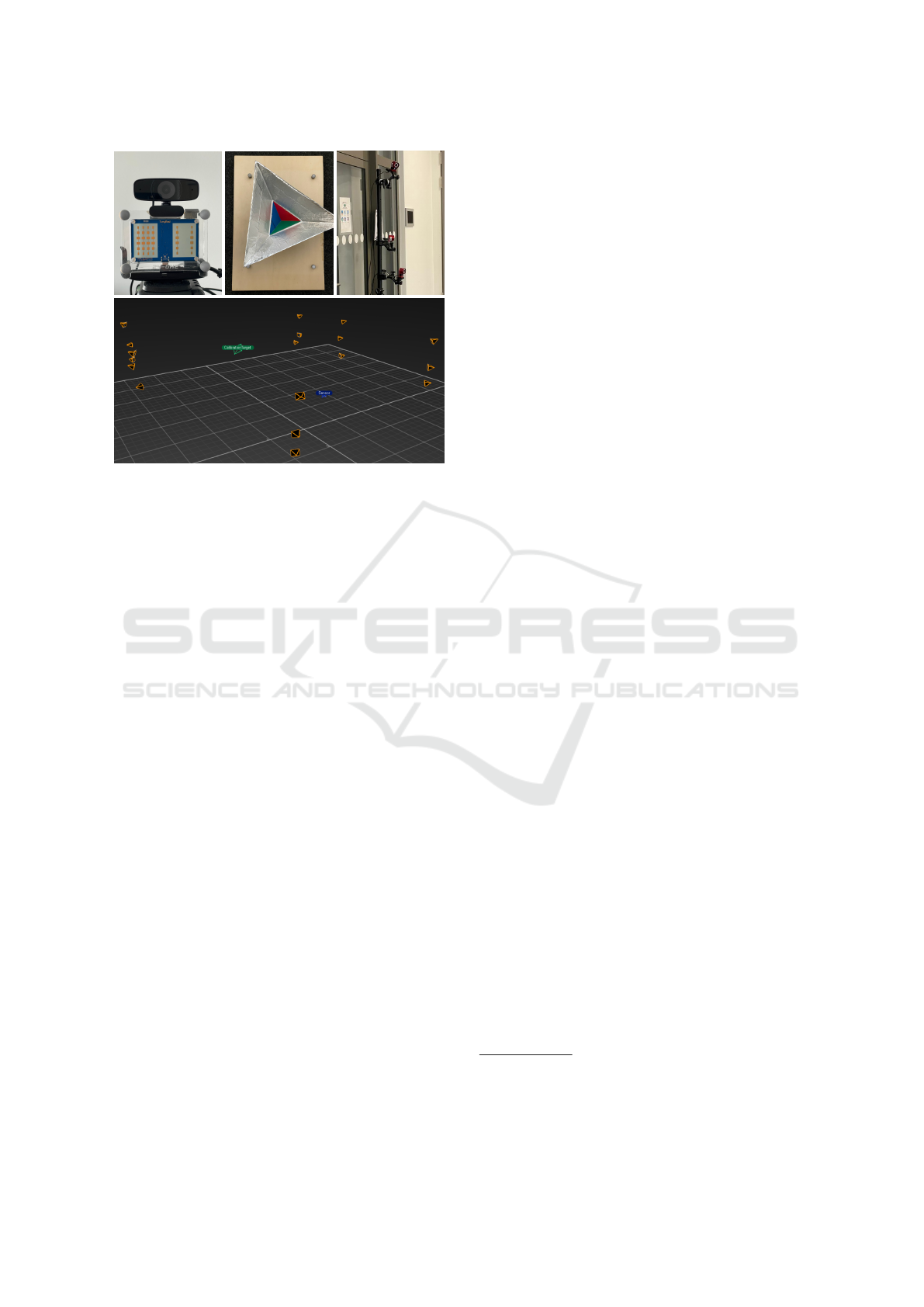
Figure 4: Top: the camera-radar setup with the reﬂective

markers, the calibration target, three OptiTrack cameras.

Bottom: OptiTrack cameras detecting the calibration target

(green) and the sensor (blue) in 3D.

where q = [q

]

⊤

= K

−1

p. To compute z

, the

equation of the sphere in Equation (8) is used in the

camera coordinate system and replacing the values for

as in Equation (15)

− x

)

+ (y

− y

)

+ (z

− z

)

= ρ

⇒z

+ q

) − 2z

+ q

)

+ (x

+ y

+ z

− ρ

) = 0.

(16)

The solution to the quadratic equation in Equa-

tion (16) yields two possible solutions. The cor-

rect solution is the one that gives a closer results of

= H

to Equation (5) with φ = π/2.

5 EVALUATION

The results of the algorithm are evaluated against the

work of El Natour et al. (El Natour et al., 2015a).

This is the only existing camera-radar 3D calibra-

tion method for 2D radar devices for static calibra-

tion. The evaluation of both methods is done for the

ﬁrst time against highly accurate ground truth mea-

surements from an optical tracker.

5.1 Ground Truth Acquisition

The evaluation calibration algorithms and 3D recon-

struction requires an accurate and precise method for

measuring the ground truth values. Therefore, an

optical motion capture (OptiTrack) system that can

achieve < 1 mm localization error is used. This sys-

tem is only used for a quantitative evaluation of the

calibration results, and not part of the calibration al-

gorithm.

Eighteen OptiTrack Flex 13

cameras are

mounted as to cover the empty space where the

calibration target is placed. Reﬂective markers are

placed on both the sensor and the calibration targets

to be detected by the cameras. Both the camera-radar

setup as well as the calibration target are visible in

the cameras’ ﬁeld of view at all times thus allowing

the accurate measurement of their relative positions.

Since the motion capture system uses infrared

light to detect the reﬂective markers, the calibration

measurements with this type of ground truth are only

possible to perform indoors for validation purposes.

5.2 Hardware Setup

The radar in use is an Analog Devices TinyRad

, this

radar is an evaluation module operating at 24 GHz

with a range resolution of 0.6 m and an azimuth reso-

lution 0.35 rad.

The camera used carries a 2 megapixels sensor ca-

pable of recording full HD images (1080p) at 30 FPS

(frames per second) with a 78

◦

FOV (ﬁeld-of-view).

The sensors are mounted with the camera on top

of the radar with a short baseline ≈ 5 cm as seen

in Figure 4.

5.3 Initialization

Knowing the difference in coordinate system orienta-

tions between the camera and radar, an initial param-

eter vector [α

,β

,γ

,0,0,0] is used to roughly align

the axes and thus speed up the convergence of the ro-

tation matrix.

While (El Natour et al., 2015a) uses stereo based

3D reconstruction to calculate their ground truth as

well as their required a priori inter-target distance,

this paper reproduces their work using the more accu-

rate OptiTrack data instead. The inter-target distance

is used to solve an optimization problem to calculate

the z

values needed to solve the main optimization

problem.

Furthermore, it was not possible to reproduce and

converge the z

solution from (El Natour et al., 2015a)

using a zero vector for initializing the optimization.

Since the original authors provide no instructions to

reproduce their work, the radar range ρ is used for

https://optitrack.com/cameras/ﬂex-13/

https://www.analog.com/en/design-center/evaluation-

hardware-and-software/evaluation-boards-kits/eval-

tinyrad.html

CaRaCTO: Robust Camera-Radar Extrinsic Calibration with Triple Constraint Optimization

539

initialization to achieve proper estimates. Another

method is to manually measure the distances which

would further complicate their approach.

5.4 Calibration Results

Different evaluation criteria are used to evaluate the

quality of the calibration both in 3D and 2D. The

convergence of the optimization is tested against dif-

ferent initializations and the quality of the calibra-

tion is evaluated against the number of measurements

needed as well as the level of noise level in the mea-

surement. In addition to that, an ablation study of the

elevation constraint is performed to show its impor-

tance.

The error in 3D is the distance between the esti-

mated 3D reprojection of the target and the ground

truth as measured by the OptiTrack system, and the

error in 2D is the distance between the projection of

the estimated 3D target and the ground truth on the

xy-plane.

5.4.1 Evaluation of the Initialization

To evaluate the effect of initialization on the cali-

bration, the optimization is performed with different

starting parameters while maintaining the same setup

in all experiments. Table 1 show that both approaches

presented in this work achieved the same average er-

rors and standard deviations for all initialization con-

ditions as well as signiﬁcantly outperformed the rival

approach. The initialization levels are deﬁned as

Best: [α

,β

,γ

,0,0,0],

Moderate: [α

,β

,γ

,0,0,0] + µ

1×6

Bad: [α

,β

,γ

,0,0,0] + ν

1×6

where µ

1−3

∈[−1 rad, 1 rad] & µ

4−6

∈ [−0.1, 0.1]

and ν

1−3

∈[−2 rad, 2 rad] & ν

4−6

∈ [−0.5, 0.5],

(17)

the components of µ and ν are uniformly sampled

from the respective ranges and added to the initial-

ization parameters described in Section 5.3. The re-

sults also show that the rival method was able to op-

timize the 2D projection on the xy−plane better than

3D space.

Our approaches show consistently better results

regardless of the initialization and both in 3D as well

as 2D projections both on the radar plane and the im-

age plane. It is also worth noting the lower standard

deviation accompanied with the lower error indicates

higher conﬁdence as well a better ﬁt to the data.

5.4.2 Evaluation of the Number of Targets

Another experiment was performed to observe the de-

pendency of the calibration algorithms on the num-

ber of measurements needed. The LM implementa-

tion (Mor

e, 1978) requires the number of residuals to

be greater than or equal to the number of parameters

to be estimated. As mentioned in Section 4.3, we are

estimating 6 parameters [α, β, γ, x

], and each

measured target position generates 3 residuals, thus a

theoretical minimum of 2 target positions are needed.

However, our experiments showed that in practice, 5

target positions are needed to converge to a valid so-

lution.

The results in Figure 5 show signiﬁcantly lower

dependency on the number of targets for our ap-

proaches and even though some improvement can be

seen with more measurements, the calibration yielded

with only 5 measurements, an error more than ﬁve

times lower than (El Natour et al., 2015a) with 36

measurements for 3D reconstruction and two times

lower for 2D. This experiment was repeated 250 times

for each n ∈ [[5, 36]] measurements randomly sampled

without replacement out of the 36 measurements. The

results are the averaged over the runs.

The poor performance of the method of El Na-

tour (El Natour et al., 2015a) on our data does not

come as a surprise if we consider that their real-

data evaluation published in (El Natour et al., 2015a)

shows an error that is a few orders of magnitude worse

than the error on simulated data. In their real-data

evaluation, (El Natour et al., 2015a) shows a mean er-

ror of 0.63 m, on a longer range and in an outdoor

setting which is less affected by multi-path interfer-

ence.

5.4.3 Simulations of Noise Levels

We simulated the effect of different levels of noise on

the reconstruction error of our calibration algorithm.

We identiﬁed three main sources of noise: radar range

measurement ρ, radar azimuth measurement θ, and

camera pixel error (u,v). In this experiment, the Opti-

Track ground truth measurements are used as a base-

line (level − 0) and deﬁne our noise levels such that

for each target i we have

= ρ

+ N (0,(0.05 × l)

= θ

+ N (0,(0.01 × l)

) = (u

+ N (0,l

),v

+ N (0,l

)),

(18)

where l is the noise level, N is the normal distribu-

tion, and l ∈ [[1,10]], and ρ

, θ

, and (u

) are

the level − 0 measurements.

ICPRAM 2024 - 13th International Conference on Pattern Recognition Applications and Methods

540

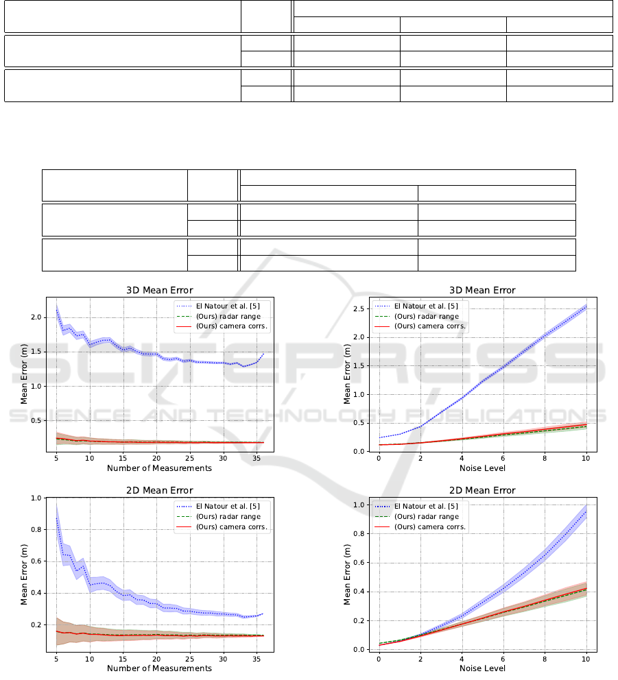
Table 1: A comparison of the mean error in meters between our method and (El Natour et al., 2015a). Different initializa-

tion setups are used to evaluate the sensitivity of the optimizations to their starting point. Where Best: [α

,β

,γ

,0,0,0],

Moderate: [α

,β

,γ

,0,0,0] + µ

1×6

∋ {µ

1−3

∈ [−1 rad,1 rad] & µ

4−6

∈ [−0.1,0.1]}, and Bad: [α

,β

,γ

,0,0,0] + ν

1×6

∋

{ν

1−3

∈ [−2 rad,2 rad] & ν

4−6

∈ [−0.5, 0.5]}.

Method Error

Initialization

Best Moderate Bad

Using camera

correspondences (ours)

3D 0.175 m ± 0.049 0.175 m ± 0.049 0.175 m ± 0.049

2D 0.129 m ± 0.065 0.129 m ± 0.065 0.129 m ± 0.065

El Natour et al. (El Natour et al., 2015a)

3D 1.474 m ± 0.640 1.474 m ± 0.640 1.606 m ± 0.440

2D 0.272 m ± 0.166 0.272 m ± 0.166 0.313 m ± 0.090

Table 2: An ablation study showing the effect of adding the constraint in Equation (13) to the optimization and the difference

between using the radar range and camera correspondences to calculate the distance to the target. The experiments were done

using the Best initialization parameters [α

,β

,γ

,0,0,0].

Method Error

Results

Without Eq. (13) constraint With Eq. (13) constraint

Using radar range

(ours)

3D 1.369 m ± 0.620 0.180 m ± 0.053

2D 0.250 m ± 0.152 0.133 m ± 0.067

Using camera

correspondences (ours)

3D 1.546 m ± 0.676 0.175 m ± 0.049

2D 0.293 m ± 0.182 0.129 m ± 0.065

Figure 5: The effect of the number of measured targets on

the result of the calibration and subsequently on the quality

of the 2D and 3D reconstruction. Our methods (overlapping

red and green) show better error even for a low number of

measurements.

Figure 6: Our methods (overlapping red and green) show

resilience to the increasing noise levels for both 2D and 3D

reconstruction and achieve a worst case of 0.5 m mean error

for 3D reconstruction. Both methods outperform (El Natour

et al., 2015a) which performs 5 times worse in 3D recon-

struction and 2 times worse in 2D reconstruction at noise

level 10.

CaRaCTO: Robust Camera-Radar Extrinsic Calibration with Triple Constraint Optimization

541

Figure 6 shows the 2D and 3D target reconstruc-

tions errors for the different noise levels. We can see

our method outperforming (El Natour et al., 2015a)

in for all levels of noise in 3D reconstruction. For 2D

reconstruction, all three methods show similar recon-

struction error for level −0 noise, however, (El Natour

et al., 2015a) quickly diverges after level − 4 noise.

This experiment was repeated 250 times for all noise

levels, and show our methods’ robustness to noise.

5.4.4 Ablation Study of the Elevation Constraint

To highlight the importance of our elevation con-

straint, deﬁned in Equation (13), we ran an ablation

study on both of our range calculation methods. This

was done using the Best initialization parameters as

described in Equation (17) and the results can be seen

in Table 2. The mean errors achieved without using

the elevation constraint are considerably higher than

the results achieved when including it. The errors

without the constraint in Equation (13) are also close

to the results of (El Natour et al., 2015a) as seen in Ta-

ble 1. This is expected because the main difference

between them is the distance calculation method. We

observe that before adding the constraint, our method

using the radar range for distance measurement per-

formed better than the method using the camera cor-

respondences, this result was reversed after adding the

constraint.

6 CONCLUSION

In this work, we introduced a new method for extrin-

sic calibration of a camera-radar system. The method

was tested against a high-accuracy motion capture

system, which served as the ground truth. Our setup

is not only simpler, as it operates independently with-

out external sensing, but it also delivers superior re-

sults. Even with less accurate initial parameters and

fewer measurement points, the additional optimiza-

tion constraints we introduced allow the calibration

to converge effectively. We also utilized the calibra-

tion output to reconstruct the 3D targets from the data

matched by the camera-radar system. Instead of more

complicated target designs, our streamlined setup re-

quires fewer calibration targets and merely uses a

single standard retroreﬂector. While our current ap-

proach only focuses on static targets, calibrating on

a moving target would likely yield better radar target

detection. However, this would come at the cost of

complicating the process, including the setup and tar-

get detection phases of our work.

ACKNOWLEDGMENT

This work has been partially funded by the Ger-

man Ministry of Education and Research (BMBF) of

the Federal Republic of Germany under the research

project RACKET (Grant number 01IW20009). Spe-

cial thanks to Stephan Krauß, Narek Minaskan, and

Alain Pagani for their insightful remarks and discus-

sions.

REFERENCES

Bian, J., Lin, W.-Y., Matsushita, Y., Yeung, S.-K., Nguyen,

T.-D., and Cheng, M.-M. (2017). Gms: Grid-based

motion statistics for fast, ultra-robust feature cor-

respondence. In Conference on Computer Vision

and Pattern Recognition (CVPR), pages 4181–4190.

IEEE.

Chavez-Garcia, R. O. and Aycard, O. (2015). Multiple sen-

sor fusion and classiﬁcation for moving object detec-

tion and tracking. IEEE Transactions on Intelligent

Transportation Systems, 17(2):525–534.

Cho, H., Seo, Y.-W., Kumar, B. V., and Rajkumar, R. R.

(2014). A multi-sensor fusion system for moving ob-

ject detection and tracking in urban driving environ-

ments. In International Conference on Robotics and

Automation (ICRA), pages 1836–1843. IEEE.

Domhof, J., Kooij, J. F., and Gavrila, D. M. (2019). An

extrinsic calibration tool for radar, camera and lidar. In

International Conference on Robotics and Automation

(ICRA), pages 8107–8113. IEEE.

El Natour, G., Aider, O. A., Rouveure, R., Berry, F., and

Faure, P. (2015a). Radar and vision sensors calibration

for outdoor 3d reconstruction. In International Con-

ference on Robotics and Automation (ICRA), pages

2084–2089. IEEE.

El Natour, G., Ait-Aider, O., Rouveure, R., Berry, F., and

Faure, P. (2015b). Toward 3d reconstruction of out-

door scenes using an mmw radar and a monocular vi-

sion sensor. Sensors, 15(10):25937–25967.

Kim, D. Y. and Jeon, M. (2014). Data fusion of radar

and image measurements for multi-object tracking via

kalman ﬁltering. Information Sciences, 278:641–652.

Lepetit, V., Moreno-Noguer, F., and Fua, P. (2009). Epnp:

An accurate o (n) solution to the pnp problem. Inter-

national journal of computer vision, 81(2):155–166.

Lucas, B. D. and Kanade, T. (1981). An iterative image

registration technique with an application to stereo vi-

sion. In Proceedings of the 7th international joint con-

ference on Artiﬁcial intelligence (IJCAI), volume 2,

pages 674–679.

Mor

e, J. J. (1978). The levenberg-marquardt algorithm: im-

plementation and theory. In Numerical analysis, pages

105–116. Springer.

Oh, J., Kim, K.-S., Park, M., and Kim, S. (2018). A com-

parative study on camera-radar calibration methods.

In International Conference on Control, Automation,

Robotics and Vision (ICARCV), pages 1057–1062.

IEEE.

ICPRAM 2024 - 13th International Conference on Pattern Recognition Applications and Methods

542

OpenCV (2023a). Camera calibration and 3d reconstruc-

tion.

OpenCV (2023b). Object detection.

Per

c, J., Markovi

c, I., and Petrovi

c, I. (2019). Extrin-

sic 6dof calibration of a radar–lidar–camera system

enhanced by radar cross section estimates evaluation.

Robotics and Autonomous Systems, 114:217–230.

Rambach, J., Pagani, A., and Stricker, D. (2021). Principles

of object tracking and mapping. In Springer Hand-

book of Augmented Reality, pages 53–84. Springer.

Roy, A., Gale, N., and Hong, L. (2009). Fusion of

doppler radar and video information for automated

trafﬁc surveillance. In 12th International Conference

on Information Fusion, pages 1989–1996. IEEE.

Roy, A., Gale, N., and Hong, L. (2011). Automated trafﬁc

surveillance using fusion of doppler radar and video

information. Mathematical and Computer Modelling,

54(1-2):531–543.

Stateczny, A., Kazimierski, W., Gronska-Sledz, D., and

Motyl, W. (2019). The empirical application of auto-

motive 3d radar sensor for target detection for an au-

tonomous surface vehicle’s navigation. Remote Sens-

ing, 11(10):1156.

Sugimoto, S., Tateda, H., Takahashi, H., and Okutomi,

M. (2004). Obstacle detection using millimeter-

wave radar and its visualization on image sequence.

In International Conference on Pattern Recognition

(ICPR), volume 3, pages 342–345. IEEE.

Wang, T., Zheng, N., Xin, J., and Ma, Z. (2011). Integrating

millimeter wave radar with a monocular vision sensor

for on-road obstacle detection applications. Sensors,

11(9):8992–9008.

Wang, X., Xu, L., Sun, H., Xin, J., and Zheng, N. (2014).

Bionic vision inspired on-road obstacle detection and

tracking using radar and visual information. In In-

ternational Conference on Intelligent Transportation

Systems (ITSC), pages 39–44. IEEE.

Wise, E., Per

c, J., Grebe, C., Petrovi

c, I., and Kelly, J.

(2021). A continuous-time approach for 3d radar-to-

camera extrinsic calibration. In International Con-

ference on Robotics and Automation (ICRA), pages

13164–13170. IEEE.

Zhang, Z. (2000). A ﬂexible new technique for camera cal-

ibration. IEEE Transactions on pattern analysis and

machine intelligence, 22(11):1330–1334.

APPENDIX

Target Matching in Camera Frames

In this section we will explain in detail the process of

automatically detecting the calibration target as well

its corners and center as required in Section 4.2.2.

This step is a decoupled problem from the calibra-

tion algorithm and other approaches are available to

achieve this task.

Figure 7: A sample input frame where the corner targets

must be detected.

Template Matching

Given a sample input frame as shown in Figure 7, it

is desired to ﬁrst ﬁnd the location of the target in the

frame to reduce the search space for feature matching

and improve its robustness.

Figure 8: (left) Patch of the calibration target to be used as

a template. (right) Masked version of the patch.

A template (Figure 8) is used to ﬁnd the candi-

date positions of the target in the input frame. Tem-

plate matching (OpenCV, 2023b) is applied to the in-

put frame with different scales and rotations of the

template. Our experiments show that masking out the

clutter around the target in the template as seen in Fig-

ure 8 yields more robust detection.

The template matching results in multiple can-

didate positions that are merged depending on their

overlap value with a vote being assigned to the

merged patch corresponding to the number of can-

didates merged at that position. The result of steps

(1) and (2) of Figure 9 shows the candidate positions

before and after merging as well as the ﬁnal selected

patch in the input frame.

Template Alignment

After ﬁnding the desired patch, we use the GMS Fea-

ture Matcher (Bian et al., 2017) to detect correspon-

dences between the template and the selected patch.

The GMS Matcher allows for more robust feature

matching between the two patches. Figure 9 shows

the result of the feature matching (3) after resizing

the patches to similar dimensions and applying edge

enhancing ﬁltering.

CaRaCTO: Robust Camera-Radar Extrinsic Calibration with Triple Constraint Optimization

543

Input Frame

Template

-1-

Template

Matching

-2-

Best

Candidate

-3-

Feature

Matching

-4-

Template

Alignment

-5-

Refine

Alignment

-6-

Find

Center

-7-

Reproject

to Input

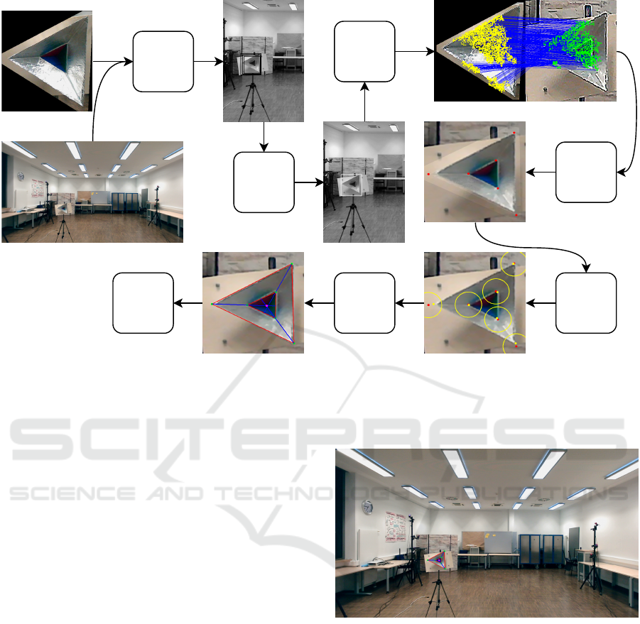
Figure 9: The complete diagram describing the detection of the target. (1) Generate candidate positions of the template

matching. (2) Find best patch location. (3) Match features between the template and the chosen patch location. (4) Align the

template to the patch, the red dots represent the known corner positions of the template. (5) Reﬁne the corner positions, the

yellow dots show the reﬁned position of the corner. (6) Calculate the center point as the intersection of the lines connecting

the corners. (7) Reproject the center to the original image.

The matched features are used to compute the

homography (OpenCV, 2023a)and align the template

to the image patch. Step (4) of Figure 9 presents

the aligned template on top of the image patch, the

red dots represent the known corner positions in the

template. The ﬁgure shows that some reﬁnement is

needed for proper alignment of the corners.

Corner Reﬁnement

To further reﬁne the position of the corners in the im-

age patch, we apply Lukas-Kanade method (Lucas

and Kanade, 1981) for sparse optical ﬂow. We as-

sume small changes in the corner position from one

image to the other and apply the method for each cor-

ner separately for more robust results. Figure 9 shows

the result of the corner reﬁnement in yellow (5), the

circle around the original red corner position has a ra-

dius of 50 pixels (image is upscaled by 3.5 times).

Center Detection

After detecting the corners on the target, the detection

of the center becomes straightforward, by connecting

the corners of both triangles and ﬁnding the mean in-

tersections between the 3 lines as seen in Figure 9.

Finally, Figure 10 shows the position of the center

point obtained in the original image.

Figure 10: The target center point projected back to the

original image.

Decoupled Noise Simulations

In addition to the experiments presented in Sec-

tion 5.4.3 on the combined noise levels, we per-

formed 3 experiments exploring the decoupled effects

of the added noise. Similar to the simulations in Sec-

tion 5.4.3, we ran the experiments 250 times for each

noise level, and averaged over the runs. The noise is

deﬁned similar to Section 5.4.3 as

= ρ

+ N (0,(0.05 × l)

= θ

+ N (0,(0.01 × l)

) = (u

+ N (0,l

),v

+ N (0,l

)),

(19)

ICPRAM 2024 - 13th International Conference on Pattern Recognition Applications and Methods

544

where l is the noise level, N is the normal distribu-

tion, and l ∈ [[1,10]], and ρ

, θ

, and (u

) are

the level − 0 measurements. For each of the experi-

ments noise is added to one of the parameters while

level − 0 noise is used for the other two.

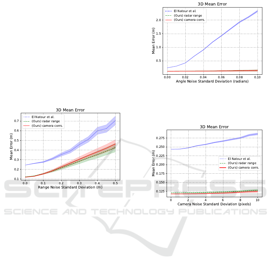
Radar Range Noise

Simulating radar range noise shows a similar increase

in 3D mean error for both our methods and (El Natour

et al., 2015a). Figure 11 shows that our methods out-

perform El Natour et al. (El Natour et al., 2015a) over

for all standard deviation values with the difference

growing slightly the larger the noise standard devia-

tion.

Figure 11: The mean error in 3D reconstruction as a func-

tion of the standard deviation of the added noise to the

range.

Radar Azimuth Noise

Figure 12 shows that noise in the radar azimuth

measurement has the biggest effect on the quality

of (El Natour et al., 2015a) while our methods are

much more robust to this type of noise. The mean re-

construction error of (El Natour et al., 2015a) shoots

to more than 2 m for a noise standard deviation of

0.1 rad while our methods maintain an error lower

than 0.25 m for the same range.

Camera Pixel Noise

Introducing noise of up to 10 pixels to all methods had

the smallest effect on all methods. While our methods

show an average increase in 3D reconstruction error

of around 1 cm, El Natour et al. (El Natour et al.,

2015a) increase by 2 to 3 cm.

Analysis of Results

The experiments show the robustness of our method

to different sources of noise with the radar range noise

Figure 12: The mean error in 3D reconstruction as a func-

tion of the standard deviation of the added noise to the az-

imuth angle. The method by El Natour et al. (El Natour

et al., 2015a) shows very high sensitivity to the azimuth

noise.

Figure 13: The mean error in 3D reconstruction as a func-

tion of the standard deviation of the added noise to the target

pixel location.

having the biggest effect on our 3D reconstruction re-

sults. On the other hand, the method in (El Natour

et al., 2015a) shows a lot of sensitivity to variations

in the radar azimuth measurements, and overall lower

accuracy of the 3D reconstruction of the measurement

targets.

CaRaCTO: Robust Camera-Radar Extrinsic Calibration with Triple Constraint Optimization

545