Counterfactual-Based Feature Importance for Explainable Regression of

Manufacturing Production Quality Measure

Antonio L. Alfeo

1,2 a

, and Mario G. C. A. Cimino

1,2 b

Dept. of Information Engineering, University of Pisa, Pisa, Italy

Research Center E. Piaggio, University of Pisa, Pisa, Italy

Keywords:

Explainable Artiﬁcial Intelligence, Expert-Based Validation, Feature Importance, Regression Problem.

Abstract:

Machine learning (ML) methods need to explain their reasoning to allow professionals to validate and trust

their predictions, and employ those in real-world decision-making processes. To do so, explainable artiﬁcial

intelligence (XAI) methods based on feature importance can be employed, even though those can be very

computationally expensive. Moreover, it can be challenging to determine whether an XAI technique might

introduce bias into the explanation (e.g., overestimating or underestimating the feature importance) in the

absence of some reference feature importance measure or even some domain knowledge from which deriving

an expected importance level for each feature. We address both these issues by (i) employing a counterfactual-

based strategy, i.e. deriving a measure of feature importance by checking if some minor changes in one

feature’s values signiﬁcantly affect the ML model’s regression outcome, and (ii) employing both synthetic and

real-world industrial data coupled with the expected degree of importance for each feature. Our experimental

results show that the proposed approach (BoCSoRr) is more reliable and way less computationally expensive

than DiCE, a well-known counterfactual-based XAI approach able to provide a measure of feature importance.

1 INTRODUCTION AND

MOTIVATIONS

Machine learning technology has become ubiquitous,

with unprecedented recognition performances (Alfeo

et al., 2017) and applications spanning across every

domain (Alfeo et al., 2019). However, since ML

approaches can work as a black box, domain ex-

perts cannot easily validate and trust their outcomes

(Alfeo et al., 2022a). This is especially important

in real-world scenarios such as in smart manufac-

turing (Alfeo et al., 2022b). The adoption of AI

technology can improve the manufacturing productiv-

ity only if the AI’s outcomes can be understood and

trusted enough to be integrated into decision-making

processes (

Ic¸ and Yurdakul, 2021). To address this

challenge, Explainable Artiﬁcial Intelligence (XAI)

methodologies can be used to provide some insights

into the reasoning of ML models (Jeyakumar et al.,

2020). Employing XAI techniques in smart manufac-

turing contexts can indeed lead to cost reduction, pre-

diction error minimization, and enhanced debugging

https://orcid.org/0000-0002-0928-3188

https://orcid.org/0000-0002-1031-1959

of AI-based systems (Ahmed et al., 2022).

The explanations provided via post-hoc XAI tech-

niques can be organized according to their scope and

form. An explanation can be local or global. Lo-

cal explanations focuses on the ML’s outcome for a

speciﬁc instance. Global explanations offer insights

into the decision process of the ML model as a whole.

Moreover, according to the recent survey (Miller,

2019), the explanations’ form can be organized into

three main groups: (i) Instance-based explanations

link a given instance to prototypes or counterfactual

examples, triggering a similarity-based reasoning for

end-users like domain experts. Given one data in-

stance, its counterfactual is a similar instance that cor-

responds to a different ML model’s outcome (Delaney

et al., 2021); (ii) Attribution-based explanations un-

fold the AI model’s decision process by evaluating

the contribution of each input feature to the predic-

tion. Attribution-based approaches can provide both

local and global explanations (Afchar et al., 2021);

and (iii) Rule-based explanations attempt to approx-

imate the decision process of the algorithm by asso-

ciating labels with input feature thresholds (van der

Waa et al., 2021). Choosing a suitable explanation

form is an application-dependent design choice. In

Alfeo, A. and Cimino, M.

Counterfactual-Based Feature Importance for Explainable Regression of Manufacturing Production Quality Measure.

DOI: 10.5220/0012369600003654

Paper published under CC license (CC BY-NC-ND 4.0)

In Proceedings of the 13th International Conference on Pattern Recognition Applications and Methods (ICPRAM 2024), pages 48-56

ISBN: 978-989-758-684-2; ISSN: 2184-4313

the context of smart manufacturing, the end-users are

typically non-experts in AI. So, highly comprehen-

sible explanations should be prioritized. In this re-

gard, attribution-based (e.g., feature importance) and

instance-based (e.g., counterfactual) explanations can

be employed (Markus et al., 2021). Speciﬁcally,

feature importance approaches are widely used due

to the availability of model-agnostic techniques that

generate feature rankings (Afchar et al., 2021). The

widespread use of these approaches has exposed their

limitations, including their great computational com-

plexity (Kumar et al., 2020). To address this limita-

tion, an increasing body of research is exploring inno-

vative strategies that combine feature importance and

counterfactual explanations (Alfeo et al., 2023b).

Furthermore, it’s well-known that the assumptions

behind the reliability of feature importance measures

may not hold in real-world scenarios. For instance,

when the features are characterized by signiﬁcant cor-

relation and co-dependence, some measures of fea-

ture importance may become unreliable (Marc

ılio and

Eler, 2020). In these cases, it’s challenging to de-

termine whether the XAI method is overestimating

or underestimating the importance of one feature. A

proper validation of a feature importance measure

would need some reference importance measure or

domain knowledge that provides an expected impor-

tance level for each feature. Unfortunately, this need

is often neglected due to the high costs and the dif-

ﬁculties associated with obtaining an a-priori quan-

titative assessment of feature informativeness (Arras

et al., 2022; Ali et al., 2023).

In this paper, we tackle this issue by leverag-

ing both synthetic and real-world datasets that in-

clude a degree of expected importance for each fea-

ture. With the synthetic dataset, the expected im-

portance of each feature is imposed by the data gen-

eration procedure (Guidotti, 2021). With the real-

world dataset, we rely on the expertise of man-

ufacturing domain professionals to obtain the ex-

pected feature importance level for each feature (Barr

et al., 2020). We employ these datasets to eval-

uate a novel efﬁcient counterfactual-based feature

importance measure for regression problems (BoC-

SoRr). The proposed method is compared to a well-

established counterfactual-based feature importance

measure from the state-of-the-art.

The structure of the paper is as follows. Section

2 presents the related works. Section 3 details the

method we propose. Section 4 covers the case stud-

ies and the experimental setup. Section 5 discusses

the results obtained, and ﬁnally, Section 6 outlines the

conclusions drawn from this study.

2 RELATED WORKS

The majority of the research works using XAI ap-

proaches employ feature importance methods (Miller,

2019). Those methods assign importance scores to

each feature based on some criteria, such as by esti-

mating the Shapley value (Sundararajan and Najmi,

2020). In contrast, counterfactual explanations are

minimally different versions of the sample whose pre-

dictions need to be explained, that results in a differ-

ent prediction.

According to (Kommiya Mothilal et al., 2021),

counterfactuals can offer an alternative means for de-

riving feature importance measures since both those

approaches focus on the model’s decision boundary.

Counterfactual approaches aim to ﬁnd the minimal

change in the data instance that results in the cross-

ing of the model’s decision boundary (Schleich et al.,

2021), whereas some feature importance measures at-

tempt to approximate it (Ribeiro et al., 2016). This

allows employing counterfactual approaches to gen-

erate new and improved procedures to measure the

feature’s importance and vice versa. Indeed, there is

a growing body of research exploring these strategies

(Alfeo et al., 2023b).

For instance, in (Wiratunga et al., 2021), the au-

thors propose an approach for generating counter-

factuals by modifying the most important features,

as measured via Shapley values. Given an instance

to be explained, the authors in (Vlassopoulos et al.,

2020) obtain a local approximation of the model’s de-

cision boundary by generating counterfactuals via a

variational autoencoder. Similarly, in (Laugel et al.,

2018) the authors generate new instances in a hyper-

sphere surrounding the sample to be explained to pro-

vide local decision rules that are consistent with the

model’s decision boundary. However, the high com-

putational cost of this approach makes it non-feasible

for datasets with a high number of features. DiCE

(Mothilal et al., 2020) stands out as a renowned ap-

proach that employs counterfactual explanations to

derive feature importance measures. DiCE generates

a set of counterfactual explanations for a given pre-

diction. By examining how the feature values change

across the counterfactuals, DiCE provides insights

into which features have the most signiﬁcant inﬂu-

ence on the prediction outcome. In short, the fea-

tures that exhibit the greatest variation in the counter-

factuals are considered more important. Considering

its established reputation and its suitability both for

classiﬁcation and regression problems (Dwivedi et al.,

2023), we select DiCE as the state-of-the-art bench-

mark for evaluating our proposed feature importance

measure.

Counterfactual-Based Feature Importance for Explainable Regression of Manufacturing Production Quality Measure

Requires:

M ⇐ trained machine learning model

M(s) ⇐ the prediction of M for instance s

I ⇐ set of all the instances in the data

F ⇐ set of all the features in the data

L ⇐ set of all the labels in the data

n ⇐ number of instances to query

k ⇐ number of counterfactuals per instance to query

Procedure:

1: relevantFeatures ⇐ emptyList()

2: instanceDist ⇐ computePairwiseDistance(I, I,Cosine similarity)

3: labelDist ⇐ computePairwiseDistance(L,L,Euclidean distance)

4: counterDist ⇐ minMax(labelDist) + minMax(instanceDist)

5: instancesToQuery ⇐ samplesWithTopAvgDist(counterDist,n)

6: For each i ∈ instancesToQuery

7: counter f actuals ⇐ samplesWithTopDist(counterDist,i,k)

8: For each c ∈ counter f actuals

9: For each f ∈ F

10: s

tmp

⇐ changeFeatureValue(i,c, f )

11: if (|M(s

tmp

) − M(i)| > |M(s

tmp

) − M(c)| )

12: relevantFeatures.append( f )

13: End if

14: End For

15: End For

16: End For

17: f eatureImportance ⇐ f requenceByFeature(relevantFeatures)

18: return f eatureImportance

Algorithm 1: Procedure to measure the feature importance (i.e., BoCSoRr).

3 DESIGN

In this section, the design of the proposed method is

detailed.

We propose the Boundary Crossing Solo Ratio

for Regression problem (BoCSoRr), a global feature

importance measure obtained by aggregating local

counterfactual explanations. This method is an

adaption for the regression problem of the method

presented in (Alfeo et al., 2023b). The method

in (Alfeo et al., 2023b) is designed for the clas-

siﬁcation domain and is based on the concept of

counterfactuals, i.e. samples characterized by minor

features change but different classes. We employ

this terminology in this study even if in this case

there are no counterfactual classes. Indeed, since we

address a regression problem the concept of counter-

factual class is replaced by a more broad “signiﬁcant

difference in the model’s outcome”. Speciﬁcally,

BoCSoRr evaluates the importance of one feature by

considering the frequency with which a slight change

in the value of that speciﬁc feature results in a sig-

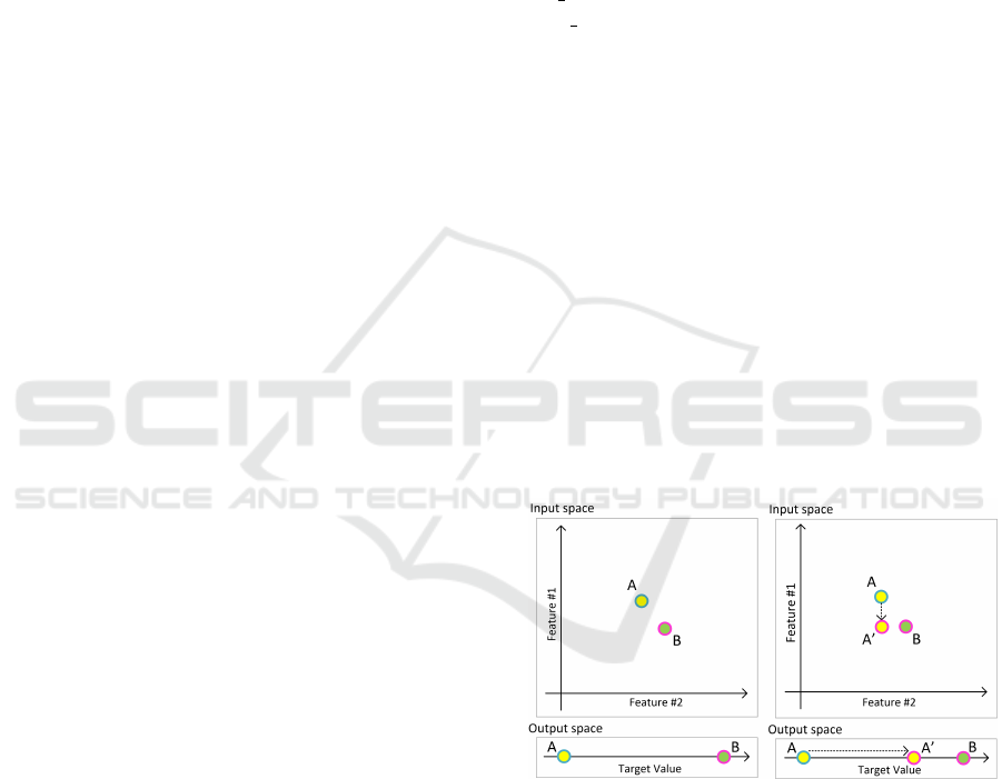
niﬁcant change in the model’s outcome (see Fig. 1).

Figure 1: Representation of the idea behind BoCSoRr’s fea-

ture relevance. Let’s consider two samples, A and B, that

are close in the input space and distant in the output space.

Sample A

′

is generated using sample A and changing the

value of Feature #1 with the one of sample B. Feature #1

can be considered relevant since, as a result of its change

alone, A

′

is closer to B than A in the output space.

To ﬁnd the samples that are close in the input

space (i.e. the feature space) and distant in the output

space (i.e. the regression target), we consider both (i)

the cosine similarity (Abbott, 2014) between all the

samples in the feature space, and (ii) the Euclidean

ICPRAM 2024 - 13th International Conference on Pattern Recognition Applications and Methods

distance of the labels (i.e. the target quantity of the

regression problem). Via a min-max procedure (Ab-

bott, 2014), we rescale between 0 and 1 both of these

quantities and aggregate those (lines 2-4 of Algorithm

1), to obtain the counterDist, a distance bounded be-

tween 0 and 2. 0 corresponds to samples pair very

far apart in the input space and with minimal dif-

ference in the output space. 2 corresponds to sam-

ple pairs very close in the input (whose values will

therefore be characterized by slight differences) and

with maximum difference in the output space. As in

(Alfeo et al., 2023b), we aim at identifying sample

pairs characterized by a great counterDist. Firstly,

we select the n samples corresponding to the greatest

average counterDist with all the samples (line 5 of Al-

gorithm 1), and then for each i instance among those,

we select the k samples with the greatest counterDist

w.r.t. i (line 7 of Algorithm 1). As introduced at the

beginning of this section, we call those samples coun-

terfactuals. The above-presented two-step search pro-

cedure is preferred to a simpler search for the pairs of

samples characterized by the greatest counterDist to

avoid populating the search result with outliers.

Then, we substitute (one at a time) the features’

value of samples i with one of its counterfactuals. If

this single value change shifts the prediction closer to

the label of the counterfactual, the modiﬁed feature is

considered relevant. The regression outcome change

is measures as the absolute value of their Euclidean

distance (lines 10-12 of Algorithm 1).

By taking into account all the samples i and their

counterfactuals, the frequency with which a feature is

considered relevant (line 17, Algorithm 1) is used as a

proxy of the importance of that feature (Vlassopoulos

et al., 2020). Algorithm 1 shows a high-level pseudo-

code of the above-described procedure.

4 EXPERIMENTAL SETUP

This section presents the experimental setup, the met-

rics used to evaluate the convenience of proposed

method, and the datasets we employed in the exper-

iments.

4.1 Synthetic Dataset

To assess the reliability of the feature importance

measure, we build a tabular dataset with predeﬁned

feature importance levels, following a methodology

similar to the ones outlined in (Barr et al., 2020) and

(Alfeo et al., 2023b).

Speciﬁcally, we employ the make regression

function from the Python library scikit-learn (Pe-

dregosa et al., 2011). This function generates the

data for a random regression problem. The tar-

get values are obtained as a random linear combi-

nation of the features, to which optional sparsity

and noise can be included (Pedregosa et al., 2011).

The make regression function allows to explicit select

how many samples to generate and how many features

should be informative (or not) in the dataset. Thus, we

build a dataset consisting of 1000 samples, with ﬁve

informative features followed by ten non-informative

ones. Also, some additional Gaussian noise is intro-

duced to each non-informative feature. The amount

of noise progressively increases from the 6th feature

to the 15th, such that those are supposed to be less

and less informative. It’s worth noting that since it

is impossible to quantify how the addition of noise

precisely diminishes the informativeness of one fea-

ture, the ground truth feature importance for this syn-

thetic dataset consists of two importance levels, high

(informative features) and low (non-informative fea-

tures). Similar to other studies that generate data with

known feature importance (Yang and Kim, 2019), the

approach used to generate the synthetic dataset allows

for comparison of the feature importance as measured

via different XAI approaches on the same features and

assess if the computed importance metrics is more or

less aligned with the expected feature importance val-

ues.

4.2 Real-World Dataset

This study employs a real-world dataset provided by

Koerber Tissue, a company specialized in the produc-

tion of industrial machines for tissue paper manufac-

turing. These machines are aimed at processing big

reels of raw paper by pressing and gluing the paper

layers while embossing a speciﬁc motif (e.g. the logo

of the seller) onto the ﬁnal product. Each machine is

tested using various paper types and production set-

tings, such as the machine speed or embossing pres-

sure (i.e., the features of our analysis). For each pro-

duction setting, multiple measurements are taken on

the ﬁnal product. These measurements encompass

quality-related measures of the ﬁnal product, such as

paper resistance and bulkiness, i.e. the target of our

analysis.

Like many real-world datasets, the company’s

data needs to be preprocessed to remove sensitive in-

formation and handle the missing values. To this aim,

all of the columns with more than 66% missing values

are removed. Then, we remove all the data instances

with more than 50% features characterized by miss-

ing values. Finally, all the data instances are clustered

according to the values of the most informative and

Counterfactual-Based Feature Importance for Explainable Regression of Manufacturing Production Quality Measure

sensitive features that do not present missing values.

For each feature, the numerical missing value of one

data instance is replaced with the median of its cluster.

The sensitive features are then removed.

The resulting dataset consists of more than 440

instances and 12 attributes (Table 1), which are: (i)

a unique identiﬁer for each test measurement (ID),

which is not considered an informative feature and

thus it is removed from the analysis; (ii) the per-

centage of elongation of the raw paper (when dry)

in the latitudinal (ELOLA) and longitudinal direction

(ELOLO); (iii) the ratio of the raw paper resistance in

the longitudinal and latitudinal directions (DRYRAT).

(iv) the hardness of the rubber top (TRH) and bot-

tom (BRH) roll used to imprint a motif on the pa-

per, and measured in Shore A; (v) the strength of

the raw paper in the latitudinal (STRLA) and longi-

tudinal direction (STRLO); (vi) the thickness of the

raw paper (THICK); (vii) the weight of the raw paper

(WEIGHT); and (viii) the number of tissue layers in

the ﬁnal product (LAYERS); (ix) the bulkiness of the

ﬁnal product (BULK), i.e. the targets of the analysis.

In order to obtain the ground truth for the feature

importance, we gathered both the experts of the tis-

sue production process and the machine data analysts.

The level of expected importance for a feature in the

data results from their agreement on how critical and

informative that feature could be for recognizing the

bulkiness of the ﬁnal product according to their expe-

rience and domain knowledge. For the purpose of this

analysis, those levels are grouped into two categories,

high and low.

Table 1: Expected feature importance level according to the

domain experts.

Attribute Units Expected Imp.

ID Integer -

ELOLA % LOW

ELOLO % LOW

DRYRAT Real LOW

TRH ShA LOW

BRH ShA LOW

STRLA N/m LOW

STRLO N/m LOW

THICK mm HIGH

WEIGHT gr/m

HIGH

LAYERS Integer HIGH

BULK Real -

4.3 Performance Evaluation

As motivated in Section 2, the proposed method is

compared with an established state-of-the-art method

that derives measures of importance from counterfac-

tuals, i.e. DiCE (Mothilal et al., 2020). All experi-

mental results are provided via 10 repeated trials, the

obtained performances are shown in aggregate form

as mean or conﬁdence interval. Each iteration in-

cludes the re-training of the ML approach and the

measurements of the feature importance. This en-

sures that different measures of feature importance

(e.g. BoCSoRr and DiCE) are actually evaluating the

same trained ML model at each iteration.

As performance measures, we ﬁrst consider the

computational cost of the proposed method. To do

so we measure the time (in seconds) required to com-

pute the feature’s importance. The smaller the com-

putation time needed to obtain the feature importance

measure, the better. All the experiments are run on

the same Google Colaboratory session, featuring an

Intel Xeon CPU with 2 vCPUs, and 13 GB RAM. To

ensure better comparability, the number of samples

used by DiCE to compute the feature importance is

constrained to those used by BoCSoRr, i.e. k times n.

Then, we consider the method’s ﬁdelity, i.e. if the

feature importance measure correctly represents the

ML model’s decision process (Coroama and Groza,

2022). The ﬁdelity can be measured by comparing

the proposed feature importance measure with a re-

liable model-based reference measure. For instance,

many ML approaches based on decision trees (Ab-

bott, 2014) do provide a built-in measure of fea-

ture importance (i.e. the Gini index (Abbott, 2014))

that can be used as a reference measure when the

ML model under analysis is indeed a decision tree.

Since any feature importance measure provides dif-

ferent importance value ranges, those can be difﬁcult

to compare by simply using a distance measure. How-

ever, feature importance approaches are often used to

derive a rank of the features, and two ranks can easily

be compared using measures like the Spearman rank

correlation coefﬁcient (Zar, 2005).

The Spearman rank correlation coefﬁcient, de-

noted as ρ, is a non-parametric measure of the

strength and direction of the monotonic relationship

between two variables. Spearman’s ρ is calculated

by ﬁrst transforming the array of data points (i.e. the

value of measured importance for each feature) into

ranks and then computing the Pearson correlation co-

efﬁcient on the ranked data. It ranges from -1 to 1,

where ρ = 1 represents a perfect increasing mono-

tonic relationship, and ρ = −1 represents a perfect

decreasing monotonic relationship.

ρ = 1 −

∑

n(n

− 1)

(1)

In (1), d

represents the difference between the ranks

of feature i, whereas n is the number of features.

ICPRAM 2024 - 13th International Conference on Pattern Recognition Applications and Methods

We employ Spearman’s ρ between the reference fea-

ture importance measure and the one obtained via the

other feature importance method as a measure of its

ﬁdelity.

Finally, we consider the empirical correctness

of the proposed method, i.e. if there is an agree-

ment between the obtained feature importance mea-

sure and the expected importance of each feature, i.e.

the ground truth (Coroama and Groza, 2022). Such

ground truth can be derived from domain experts’

knowledge (Alfeo et al., 2022b) or available by de-

sign if the data are generated according to some pre-

deﬁned level of importance (Guidotti, 2021). Simi-

larly to the proposal in (Alfeo et al., 2023a), to mea-

sure the agreement between the ranking of the fea-

tures obtained via a feature importance measure and

the ground truth, we group the ranked features accord-

ing to the number of features with a given expected

importance level. Since both the datasets used in this

study feature two levels of expected importance, we

can simply consider the highest features in the rank

as important and the rest as non-important. For in-

stance, if there are 5 important features according to

the ground truth, the top 5 features according to the

computed feature importance measure are labeled as

“important”, whereas the remaining features are con-

sidered “non-important”. Then, as the measure of em-

pirical correctness, we consider the percentage of the

features that are correctly assigned to the ground truth

importance level. This measure is bounded between

0 (worst case) and 1 (best case). As suggested in

(Coroama and Groza, 2022), and we call it empirical

correctness since it is based on a knowledge-driven

a-priori assumption on the informativeness of each

feature for the regression problem.

Given the different metrics considered in our anal-

ysis, we performed a manual exploration of BoC-

SoRr’s hyperparameter space (i.e. k and n), aiming

to strike a good trade-off among those. After exten-

sive experimentation within the range of 3 to 20, the

best trade-off is identiﬁed as k=19 and n=15 for the

real data, and k=15 and n=10 for the synthetic data.

5 RESULTS AND DISCUSSION

Being a model-agnostic feature importance measure,

BoCSoRr can be used with any ML method that han-

dles tabular data. In this research, our primary objec-

tive is to explain the ML regression model rather than

striving for optimal regression performance. As such,

for all of our experimentation, we employed a shal-

low ML approach, i.e. the Decision Tree regressor,

parametrized using the default values provided by the

scikit-learn library (Pedregosa et al., 2011).

The Decision Tree regressor (Abbott, 2014) is an

ML method used to predict a numerical value. This

model creates a tree-like structure of rules by dividing

the data into decision nodes. These splits are based

on the values of one feature, and the “purity” (mea-

sured via the Gini Index) of the data groups resulting

from the split. During tree construction, the Decision

Tree keeps track of how variables inﬂuence the re-

duction of the Gini Index. Variables that signiﬁcantly

contribute to reducing the Gini Index are considered

more important. Once trained, the Decision Tree pro-

vides a built-in measure of feature importance com-

puted by summing the Gini Index reductions for a

variable across all the splits it’s involved in. This

measure will be used to evaluate the ﬁdelity of the

proposed method.

We computed the feature importance for the syn-

thetic data by employing both DiCE and BoCSoRr.

In Fig. 2, the solid line represents the average feature

importance measure obtained via BoCSoRr, whereas

the dashed line represents the average feature impor-

tance measure provided by DiCE. Their values are

rescaled via a min-max procedure to better compare

them visually. The background color indicates the

expected feature importance, with the initial ﬁve fea-

tures being deemed signiﬁcant (indicated by a green

background), and subsequent non-informative fea-

tures, resulting in less and less expected importance

due to the introduction of noise (transitioning from

green to red). The resulting average feature impor-

tance measures provided by BoCSoRr exhibit a bet-

ter consistency with the expected feature importance

since it does result in lower importance for the non-

informative features (i.e. from the 6th to the 15th)

and an overall greater measured importance with the

informative ones. On the other hand, DiCE seems to

provide very small importance to the 5th feature (an

informative one) and greater importance to the 11th

feature (a non-informative one).

Figure 2: Feature importance obtained via DiCE and BoC-

SoRr with the synthetic dataset. Their values are rescaled

via a min-max procedure to better compare them visually.

The dashed line represent the separation between informa-

tive and non-informative features.

Counterfactual-Based Feature Importance for Explainable Regression of Manufacturing Production Quality Measure

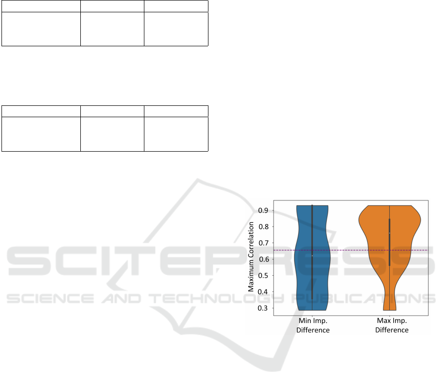
Table 2: 95% conﬁdence interval of the performance evalu-

ation measures obtained with ten repeated trials on the syn-

thetic dataset. All the rank correlation (i.e. the measure of

ﬁdelity) values corresponds to p-values lower than 0.05.

Measure BoCSoRr DiCE

Fidelity [ρ] 0.79 ± 0.03 0.72 ± 0.08

Empirical c. [%] 0.95 ± 0.05 0.88 ± 0.03

Comput. time [s] 31.45 ± 3.48 64.33 ± 3.54

Table 3: 95% conﬁdence interval of the performance evalu-

ation measures obtained with ten repeated trials on the real-

world dataset. All the rank correlation (i.e. the measure of

ﬁdelity) values corresponds to p-values lower than 0.05.

Measure BoCSoRr DiCE

Fidelity [ρ] 0.73 ± 0.06 0.23 ± 0.18

Empirical c. [%] 0.66 ± 0.07 0.58 ± 0.08

Comput. time [s] 20.97 ± 0.87 39.10 ± 0.75

We computed the performance measures pre-

sented in Section 4.3 with the synthetic data. As

evident from the results in Table 2, compared to

DiCE, BoCSoRr offers (i) signiﬁcantly less compu-

tation time, i.e. less than half the one required for

DiCE to compute the feature importance; (ii) greater

ﬁdelity, which means a greater agreement between

the feature importance ranks obtained via the built-

in feature importance measure of Decision Tree and

the ranks obtained via BoCSoRr, thus BoCSoRr bet-

ter captures the decision process of the decision tree;

and (iii) greater empirical correctness, which means

a greater agreement between the feature importance

ranks obtained via BoCSoRr and the expected feature

importance as per the synthetic data construction pro-

cedure. The last result was anticipated by the qualita-

tive evaluation provided with the results in Fig. 2.

With the real-world industrial dataset, the deci-

sion tree results in good regression performance, with

an average Mean Square Error of 0.0065 while pre-

dicting the value of the paper’s bulkiness. Then, we

explain the trained decision tree with BoCSoRr and

DiCE. By considering the performance measures de-

scribed in Section 4.3, BoCSoRr provides better re-

sults than those obtained by DiCE, with each consid-

ered performance measure (see Table 3).

Compared to the results obtained with the syn-

thetic data, between BoCSoRr and DiCE there is a

greater difference in terms of ﬁdelity and a smaller

difference in terms of computation time. Since BoC-

SoRr and DiCE use the same number of samples to

compute feature importance (see Section 4.3), the lat-

ter result can be interpreted as better scalability of

BoCSoRr with respect to the number of features. In

fact, as the number of features increases, BoCSoRr

consistently outperforms DiCE in terms of percent-

age improvement. On the other hand, the difference

in terms of ﬁdelity requires further investigation. It

is well-known from the literature that the correla-

tion between features may affect the measurement

of their importance for the ML model (Marc

ılio and

Eler, 2020). Thus, any misalignment between feature

importances should also be analyzed considering the

correlation between the features. To analyze how the

considered feature importance measures are affected

by the features’ correlation, we computed the maxi-

mum correlation (MC) between each feature and any

other feature in the dataset. Then, we select the ﬁve

features characterized by the most similar importance

value according to BoCSoRr and DiCE. To ensure

the comparability the importance values measured by

BoCSoRr and DiCE are rescaled via a min-max pro-

cedure. We repeat this procedure to identify the ﬁve

features characterized by the most dissimilar impor-

tance values according to BoCSoRr and DiCE. The

violin plots in Fig. 3 illustrate the MC values obtained

for these two groups of features.

Figure 3: The MC of the 5 features characterized by the

most similar and dissimilar importance scores provided by

BoCSoRr and DiCE, with the real-world industrial dataset.

The dotted line represent the average MC with all the fea-

tures.

According to the results shown in Fig. 3, the group

of features characterized by the greater importance

difference as measured via DiCE and BoCSoRr is

characterized by a greater MC. Overall, their average

MC is even greater than the average MC among all the

features of the whole dataset (the dashed line in Fig.

3). Vice versa for the features of the other group. In

short, BoCSoRr is more reliable than DiCE, and they

mostly disagree on the features that are more corre-

lated with any other feature of the dataset. This may

suggest that the difference both in terms of empiri-

cal correctness and ﬁdelity can be motivated by the

greater robustness of BoCSoRr to feature correlation.

ICPRAM 2024 - 13th International Conference on Pattern Recognition Applications and Methods

6 CONCLUSION

We have introduced a novel model-agnostic measure

of global feature importance for regression problems,

namely BoCSoRr. BoCSoRr broadly utilizes the con-

cept of counterfactuals and applies it to regression

problems, to determine which features, if modiﬁed,

are most likely to result in a signiﬁcant change in the

ML model’s outcome. In our experiments, we em-

ployed both synthetic and real-world data and com-

pared BoCSoRr performances against the ones ob-

tained via DiCE, a well-known counterfactual ap-

proach able to derive a feature importance measure.

With both datasets, BoCSoRr is more reliable and

less computationally expensive than DiCE. The relia-

bility of BoCSoRr is tested both in terms of ﬁdelity,

i.e. agreement with the model build-in feature impor-

tance measure, and by employing some human-driven

domain knowledge about the expected importance of

each feature for the regression problem.

As future research directions, BoCSoRr will be

employed with other ML regression approaches with

a built-in feature importance measure. This would

provide a better understanding of whether the prop-

erties proven in this study are consistent despite the

ML model used.

ACKNOWLEDGEMENTS

Work partially supported by (i) the company Koerber

Tissue in the project “Data-driven and Artiﬁcial In-

telligence approaches for Industry 4.0”; (ii) the Uni-

versity of Pisa, in the framework of the PRA 2022

101 project “Decision Support Systems for territo-

rial networks for managing ecosystem services”; the

European Commission under the NextGenerationEU

programs: (iii) Partenariato Esteso PNRR PE1 -

”FAIR - Future Artiﬁcial Intelligence Research” -

Spoke 1 ”Human-centered AI”; (iv) PNRR - M4

C2, Investment 1.5 ”Creating and strengthening of

”innovation ecosystems”, building ”territorial R&D

leaders”, project ”THE - Tuscany Health Ecosys-

tem”, Spoke 6 ”Precision Medicine and Personal-

ized Healthcare”. (v) National Sustainable Mobility

Center CN00000023, Italian Ministry of University

and Research Decree n. 1033—17/06/2022, Spoke

10; and (vi) the Italian Ministry of Education and

Research (MUR) in the framework of the FoReLab

project (Departments of Excellence), in the frame-

work of the ”Reasoning” project, PRIN 2020 LS Pro-

gramme, Project number 2493 04-11-2021, and in

the framework of the project ”OCAX -Oral CAncer

eXplained by DL-enhanced case-based classiﬁcation”

PRIN 2022 code P2022KMWX3. The authors thank

Tommaso Nocchi for his work on the subject during

his master’s thesis.

REFERENCES

Abbott, D. (2014). Applied predictive analytics: Principles

and techniques for the professional data analyst. John

Wiley & Sons.

Afchar, D., Guigue, V., and Hennequin, R. (2021). Towards

rigorous interpretations: a formalisation of feature at-

tribution. In International inproceedings on Machine

Learning, pages 76–86. PMLR.

Ahmed, I., Jeon, G., and Piccialli, F. (2022). From artiﬁcial

intelligence to explainable artiﬁcial intelligence in in-

dustry 4.0: a survey on what, how, and where. IEEE

Transactions on Industrial Informatics, 18(8):5031–

5042.

Alfeo, A. L., Cimino, M. G., Lepri, B., Pentland, A. S., and

Vaglini, G. (2019). Assessing refugees’ integration

via spatio-temporal similarities of mobility and call-

ing behaviors. IEEE Transactions on Computational

Social Systems, 6(4):726–738.

Alfeo, A. L., Cimino, M. G., and Vaglini, G. (2022a).

Degradation stage classiﬁcation via interpretable fea-

ture learning. Journal of Manufacturing Systems,

62:972–983.

Alfeo, A. L., Cimino, M. G. C., Egidi, S., Lepri, B.,

Pentland, A., and Vaglini, G. (2017). Stigmergy-

based modeling to discover urban activity patterns

from positioning data. In Social, Cultural, and Behav-

ioral Modeling: 10th International Conference, SBP-

BRiMS 2017, Washington, DC, USA, July 5-8, 2017,

Proceedings 10, pages 292–301. Springer.

Alfeo, A. L., Cimino, M. G. C., and Gagliardi, G. (2023a).

Matching the expert’s knowledge via a counterfactual-

based feature importance measure. In Proceedings

of the 5th XKDD Workshop - European Conference

on Machine Learning and Principles and Practice

of Knowledge Discovery in Databases (ECML-PKDD

2023).

Alfeo, A. L., Cimino, M. G. C. A., and Gagliardi, G.

(2022b). Concept-wise granular computing for ex-

plainable artiﬁcial intelligence. Granular Computing,

pages 1–12.

Alfeo, A. L., Zippo, A. G., Catrambone, V., Cimino, M. G.,

Toschi, N., and Valenza, G. (2023b). From local coun-

terfactuals to global feature importance: efﬁcient, ro-

bust, and model-agnostic explanations for brain con-

nectivity networks. Computer Methods and Programs

in Biomedicine, 236:107550.

Ali, S., Abuhmed, T., El-Sappagh, S., Muhammad, K.,

Alonso-Moral, J. M., Confalonieri, R., Guidotti, R.,

Del Ser, J., D

ıaz-Rodr

ıguez, N., and Herrera, F.

(2023). Explainable artiﬁcial intelligence (xai): What

we know and what is left to attain trustworthy artiﬁcial

intelligence. Information Fusion, page 101805.

Arras, L., Osman, A., and Samek, W. (2022). Clevr-xai:

a benchmark dataset for the ground truth evaluation

Counterfactual-Based Feature Importance for Explainable Regression of Manufacturing Production Quality Measure

of neural network explanations. Information Fusion,

81:14–40.

Barr, B., Xu, K., Silva, C., Bertini, E., Reilly, R., Bruss,

C. B., and Wittenbach, J. D. (2020). Towards ground

truth explainability on tabular data. arXiv preprint

arXiv:2007.10532.

Coroama, L. and Groza, A. (2022). Evaluation metrics

in explainable artiﬁcial intelligence (xai). In Inter-

national Conference on Advanced Research in Tech-

nologies, Information, Innovation and Sustainability,

pages 401–413. Springer.

Delaney, E., Greene, D., and Keane, M. T. (2021). Instance-

based counterfactual explanations for time series clas-

siﬁcation. In International inproceedings on Case-

Based Reasoning, pages 32–47. Springer.

Dwivedi, R., Dave, D., Naik, H., Singhal, S., Omer, R., Pa-

tel, P., Qian, B., Wen, Z., Shah, T., Morgan, G., et al.

(2023). Explainable ai (xai): Core ideas, techniques,

and solutions. ACM Computing Surveys, 55(9):1–33.

Guidotti, R. (2021). Evaluating local explanation methods

on ground truth. Artiﬁcial Intelligence, 291:103428.

Ic¸, Y. T. and Yurdakul, M. (2021). Development of a new

trapezoidal fuzzy ahp-topsis hybrid approach for man-

ufacturing ﬁrm performance measurement. Granular

Computing, 6(4):915–929.

Jeyakumar, J. V., Noor, J., Cheng, Y.-H., Garcia, L., and

Srivastava, M. (2020). How can i explain this to you?

an empirical study of deep neural network explanation

methods. Advances in Neural Information Processing

Systems, 33:4211–4222.

Kommiya Mothilal, R., Mahajan, D., Tan, C., and Sharma,

A. (2021). Towards unifying feature attribution and

counterfactual explanations: Different means to the

same end. In Proceedings of the 2021 AAAI/ACM

Conference on AI, Ethics, and Society, pages 652–

663.

Kumar, I. E., Venkatasubramanian, S., Scheidegger, C., and

Friedler, S. (2020). Problems with shapley-value-

based explanations as feature importance measures.

In International in proceedings on Machine Learning,

pages 5491–5500. PMLR.

Laugel, T., Renard, X., Lesot, M.-J., Marsala, C., and De-

tyniecki, M. (2018). Deﬁning locality for surrogates in

post-hoc interpretablity. In Workshop on Human Inter-

pretability for Machine Learning (WHI)-International

Conference on Machine Learning (ICML).

Marc

ılio, W. E. and Eler, D. M. (2020). From explanations

to feature selection: assessing shap values as feature

selection mechanism. In 2020 33rd SIBGRAPI confer-

ence on Graphics, Patterns and Images (SIBGRAPI),

pages 340–347. Ieee.

Markus, A. F., Kors, J. A., and Rijnbeek, P. R. (2021).

The role of explainability in creating trustworthy ar-

tiﬁcial intelligence for health care: a comprehensive

survey of the terminology, design choices, and eval-

uation strategies. Journal of Biomedical Informatics,

113:103655.

Miller, T. (2019). Explanation in artiﬁcial intelligence: In-

sights from the social sciences. Artiﬁcial intelligence,

267:1–38.

Mothilal, R. K., Sharma, A., and Tan, C. (2020). Explaining

machine learning classiﬁers through diverse counter-

factual explanations. In Proceedings of the 2020 con-

ference on fairness, accountability, and transparency,

pages 607–617.

Pedregosa, F., Varoquaux, G., Gramfort, A., Michel, V.,

Thirion, B., Grisel, O., Blondel, M., Prettenhofer,

P., Weiss, R., Dubourg, V., Vanderplas, J., Passos,

A., Cournapeau, D., Brucher, M., Perrot, M., and

Duchesnay, E. (2011). Scikit-learn: Machine learning

in Python. Journal of Machine Learning Research,

12:2825–2830.

Ribeiro, M. T., Singh, S., and Guestrin, C. (2016). ” why

should i trust you?” explaining the predictions of any

classiﬁer. In Proceedings of the 22nd ACM SIGKDD

international conference on knowledge discovery and

data mining, pages 1135–1144.

Schleich, M., Geng, Z., Zhang, Y., and Suciu, D. (2021).

Geco: quality counterfactual explanations in real time.

Proceedings of the VLDB Endowment, 14(9):1681–

1693.

Sundararajan, M. and Najmi, A. (2020). The many shapley

values for model explanation. In International confer-

ence on machine learning, pages 9269–9278. PMLR.

van der Waa, J., Nieuwburg, E., Cremers, A., and Neer-

incx, M. (2021). Evaluating xai: A comparison of

rule-based and example-based explanations. Artiﬁcial

Intelligence, 291:103404.

Vlassopoulos, G., van Erven, T., Brighton, H., and

Menkovski, V. (2020). Explaining predictions by

approximating the local decision boundary. arXiv

preprint arXiv:2006.07985.

Wiratunga, N., Wijekoon, A., Nkisi-Orji, I., Martin, K.,

Palihawadana, C., and Corsar, D. (2021). Actionable

feature discovery in counterfactuals using feature rel-

evance explainers. CEUR Workshop Proceedings.

Yang, M. and Kim, B. (2019). Benchmarking attribu-

tion methods with relative feature importance. arXiv

preprint arXiv:1907.09701.

Zar, J. H. (2005). Spearman rank correlation. Encyclopedia

of biostatistics, 7.

ICPRAM 2024 - 13th International Conference on Pattern Recognition Applications and Methods