Predicting the Level of Co-Activation of One Muscle Head from the

Other Muscle Head of the Biceps Brachii Muscle by Linear Regression

and Shallow Feedforward Neural Networks

Nils Grimmelsmann

1,2,∗ a

, Malte Mechtenberg

1,2 b

, Markus Vieth

3 c

, Alexander Schulz

3 d

Barbara Hammer

3 e

and Axel Schneider

1,2 f

Biomechatronics and Embedded Systems Group, University of Applied Sciences and Arts, Bielefeld, Germany

Institute of System Dynamics and Mechatronics, University of Applied Sciences and Arts, Bielefeld, Germany

Machine Learning Group, Bielefeld University, Bielefeld, Germany

Keywords:

sEMG, Muscle Model, Limb Movement Prediction, Virtual Sensor, Linear Regression, Regression.

Abstract:

One of the challenges in close-to-body robotics is the intuitive control of exoskeletal devices which requires

lag-free responses of its actuated joints. A frequently used signal domain to satisfy the required control

properties is surface electromyography (sEMG). By using a Hill-type model of the muscle mainly responsible

for the movement of a biological joint, which is excited by the corresponding sEMG of this muscle, the joint

movement can be pre-calculated. If the muscle internal delays are used, this information can be used for an

intuitive and lag-free control. So far, biomechanical limb and joint models including Hill-type muscle sub-

model were used. In current studies, state-of-the-art machine learning models are evaluated for this problem.

Both types, classical and machine learning models, depend on the measured sEMG signals of all muscle heads

of a relevant muscle and on their respective signal quality.

This work introduces a method to train a virtual sEMG-sensor as a replacement for the real sEMG signal of

a muscle head, thus reducing the number of real sensor electrodes on a given muscle. The virtual sensor is

trained based on data from the remaining sensor. This method allows to compare the measured sEMG signal

with the virtual sensor output to assess the measured signal. Furthermore, this study explains the training

process and evaluates the use of the virtual sensor in a biomechanical limb model.

1 INTRODUCTION

The use of active exoskeletons and wearables

provides a way to support the wearer during force-

intensive movements. This requires time critical

motion prediction so that the active exoskeleton

can be controlled in a way to follow the postures

of the wearer without delay. Electromyography

(EMG) signals provide a source of information for

the required movement prediction which can also

be measured before the muscle contracts and an

actual limb movement or force interaction with the

https://orcid.org/0000-0002-4864-4978

https://orcid.org/0000-0002-8958-0931

https://orcid.org/0000-0003-1707-6231

https://orcid.org/0000-0002-0739-612X

https://orcid.org/0000-0002-0935-5591

https://orcid.org/0000-0002-6632-3473

exoskeleton occurs. EMG signals can be measured

invasively with needles inserted into the muscle

(Merletti and Farina, 2008). This method requires

special medical knowledge on the correct insertion of

the needle into the muscle. It provides measurements

that are less affected by crosstalk, so the signal

amplitude from the selected muscle head is higher

than that from the surrounding muscle heads. The

surface electromyography (sEMG), on the other hand,

requires no special medical knowledge and is non-

invasive. Measuring EMG on the surface of the

skin means that only superﬁcial muscles or muscle

heads can be measured. Muscles or muscle heads

that lie deep below other muscle tissue are less

accessible with this measurement method. Therefore,

not all muscles or muscle heads involved in a limb

movement can be used in a model to predict the limb

movement when sEMG is the source of information.

Grimmelsmann, N., Mechtenberg, M., Vieth, M., Schulz, A., Hammer, B. and Schneider, A.

Predicting the Level of Co-Activation of One Muscle Head from the Other Muscle Head of the Biceps Brachii Muscle by Linear Regression and Shallow Feedforward Neural Networks.

DOI: 10.5220/0012368700003657

Paper published under CC license (CC BY-NC-ND 4.0)

In Proceedings of the 17th International Joint Conference on Biomedical Engineering Systems and Technologies (BIOSTEC 2024) - Volume 1, pages 611-621

ISBN: 978-989-758-688-0; ISSN: 2184-4305

611

For example, if the movement of the forearm

is considered via the elbow joint, which has one

rotatory degree of freedom, mainly three muscles are

used for ﬂexing: the two-headed biceps brachii, the

single-headed brachioradialis and the single-headed

brachialis. The extension of the elbow is mainly

performed by two muscles: the three-headed triceps

brachii and the single-headed anconeus.

The two biceps heads (biceps short head and

biceps long head) are located below the skin surface.

Both muscle heads end distally in a common tendon.

Proximally, each muscle head ends in its own tendon.

The tendons terminate at different points on the

shoulder bone, called scapular. Both heads can

ﬂex the elbow but also have secondary functions.

The proximal tendon of the biceps long head wraps

around the shoulder joint and stabilises the shoulder

(Sch

unke et al., 2010).

As shown in previous work, limb movement can

be predicted with only the two surface muscles biceps

and triceps. Firstly, with a biomechanical limb model

based on a Hill-type (Hill, 1964; Zajac, 1989) muscle

model (Grimmelsmann et al., 2023). Secondly, with

a purely data-driven (black box) approach (Leserri

et al., 2022). Depending on the experiment and data

set, a different set of the ﬁve main muscles involved

in the ﬂexion and extension of the elbow are used

for elbow movement prediction (e.g. (Koo and Mak,

2005) uses biceps, brachioradialis and the tricpes).

However, this work also shows that the signal

quality and signal integrity can be different for two

muscle heads of the same muscle, e.g. due to

changing quality of the respective electrode skin

contact. This can potentially lead to a failed

prediction depending on the overall model structure.

Due to the common distal tendon, both biceps

heads show similarities in the time courses of their

respective neuronal activation.

For this reason, a method is proposed that exploits

the close similarity between the two biceps heads

to create a virtual sensor for one head based only

on the meassurement of the sEMG of the other.

This allows the use of only one sensor, namely the

one with the better signal quality. In principle,

the concept of a virtual sensor is also suited to

derive unavailable sEMG measurements, e.g. of

deep lying muscle heads, from easy to measure more

superﬁcially located muscle heads, if their common

function suggests a similar activation in terms of time.

To test the concept of a virtual sensor, this work

follows the former of the above two applications and

replaces one of the two biceps heads, although sEMG

measurements of both superﬁcially located heads are

available. Here, the unknown signal quality of the

two measured heads is an additional challenge (see

above). The signal of the virtual sensor for one head is

derived by linear regression and shallow feedforward

neural network (FFN) using the measurement of the

other head. To reﬂect the secondary functions of the

two heads, additional features are added as input to

the regression. These additional features are related

to the dynamics of the elbow and are the elbow angle,

the upper arm angle (w.r.t. the gravitational vector)

and the overall weight of lower arm plus hand and an

additional weight (dumb bell). After the regression

step, these virtual sensors are also used as input to

the biomechanical limb model (domain-knowledge

based model) to prove the suitability for the limb

movement prediction. In previous works, different

strategies were used to train virtual sensors. One

approach is to use recurrent neural network (RNN)

such as long short-term memory (LSTM) to estimate

the virtual sEMG channel (Machado et al., 2019).

This approach focuses mainly on the performance

w.r.t. the classiﬁcation of a hand movement and

not on the interpretation of the underlying sEMG

data. The method proposed in this work uses linear

regression and shallow FFN.

Based on an extensive data set (Mechtenberg

et al., 2023), the outputs of the virtual sensor can

be compared with the neuronal activation calculated

from the real sEMG measurements of the replaced

muscle head on the one hand and evaluated w.r.t

their contribution to the predicted joint movement

on the other hand, as the virtual sensor output is

fed into the model instead of the replaced head. To

maintain interpretability the architecture/ complexity

is gradually extended in this work. Besides

interpreting the results of the virtual sensor, the sensor

is also validated using a domain-knowledge based

model.

Other methods such as (Kim et al., 2019) use

virtual sensors for a signal-assisted classiﬁcation.

The general idea of using a trained regression for

enhancing the signal integrity matches parts of our

approach (sEMG assessment).

The methods section starts with an overview of

the sEMG data set and the biomechanical model of

the upper arm and the elbow joint. The internal

signal neuronal activation from this model serves as

a foundation for the domain knowledge-based feature

used in the regression (section 2.2). A description of

the different regression setups follows in section 2.3

and section 2.4. The virtual sensor will be used in a

domain knowledge-based model. The explanation of

the validation process for this purpose can be found

in section 2.5. The methods section ends with an

exemplary use case of the virtual sensor, the sEMG

BIOSIGNALS 2024 - 17th International Conference on Bio-inspired Systems and Signal Processing

612

post measurement assessment. The results of the two

setups are discussed in section 3.1 and section 3.2.

The results section also shows the validation results

and the assessment for two different subjects.

2 METHODS

As a basis for understanding the nature of the data

on which this study is based on (Mechtenberg et al.,

2023), a brief summary of the experiments used to

collect the data is given ﬁrst. In these experiments,

the sEMG of both biceps and the two triceps heads

were recorded. The sEMG signals contain frequency

components from about 10 Hz to 400 Hz (Merletti

et al., 2018).

The periodic movement of the elbow (dumbbell

curls), however, is at about 0.5 Hz. Because of

this large difference in dynamics, the sEMG was

not directly used as the target value of the virtual

sensor regression. It is further converted into the

activation of the muscle. In the domain model, this is

achieved by a nonlinear low-pass ﬁlter that represents

the activation dynamics of the muscle head (Zajac,

1989). The resulting signal thus has lower frequency

components than the sEMG. The calculation of this

activation dynamics is brieﬂy described in section 2.2.

In sections 2.3 and 2.4 a description of the two setups

for learning the virtual sensor is presented. For

validation of the virtual sensor, the sensor is used

as a replacement input in a domain-knowledge based

model (described in section 2.5). At the end of the

methods section a potential use case (the sEMG post-

measurement assessment) of the trained virtual sensor

is described (see section 2.6).

2.1 sEMG Data Set and Biomechanical

Overview

The used data set (Mechtenberg et al., 2023) involved

31 healthy subjects performing different motion

sequences, with 29 choosing their right arm as their

dominant arm and 2 choosing the left arm. They

were randomly labeled with an identiﬁcation number

(subject id) starting from id=20. The subject ids

[23, 27, 35] were not assigned. The positions of the

acromion at the shoulder and the lateral epicondyle at

the elbow were used as reference points to calculate

the length of the upper arm. The positions of the

medial epicondyle and the processus styloideus ulnae

at the wrist were used to calculate the length of the

forearm.

Two wireless sEMG sensors (Delsys Trigno,

Delsys, Inc., Boston, MA, USA) were attached to

the skin surface above the biceps brachii and triceps

brachii. The sensors used a sampling period of

900µs and 16-bit resolution. The sensors were

applied such that their electrodes were placed on

the muscle belly proximal to the innervation zone.

The individual muscle heads of biceps and triceps

were palpated by an experienced experimenter. A

schematic representation of the two biceps heads is

shown in ﬁg. 1 (D). After the skin preparation and

alignment, the sensors were attached to the subjects’

skin with double-sided adhesive tape. The electrical

quality of the interface between the skin and the

electrodes was evaluated in a preliminary experiment

by instructing the subjects to contract the ﬂexors and

extensors of the upper arm while the experimenter

visually checked the signal quality.

A passive measurement orthosis was used to

measure the elbow angle θ synchronously with sEMG

recordings. The orthosis was custom-designed and

3D-printed in-house from PLA plastic so that it

could be adapted to different arm sizes. The elbow

angle was determined using a 10-bit magnetic rotary

position encoder (AS5043, ams AG, Premstaetten,

Austria) integrated into the joint and aligned to the

subject’s rotary axis of the elbow joint. The analog

output was fed into a Trigno Analog Adapter for

synchronous recording. Calibration was performed

by the supervisor during the initial experiment.

Figure 1(A) shows the measurement orthesis as well

as the sEMG sensors.

All subjects performed the same movement

sequences, which involved periodic movements of

the dominant forearm. Two different postures of the

upper arm were adopted and two different weighted

dumbbells were used, which were held by the subject.

The subjects were instructed to align the longitudinal

axis of the forearm orthogonally to the longitudinal

axis of the upper arm, resulting in an initial elbow

angle of θ

= 90

◦

. In the lower posture (see ﬁg. 1

(B), the upper arm was held vertically pointing

downwards. In the upper posture, the upper arm was

held vertically pointing upwards. For this study, only

the lower posture (ﬂexor muscles dominant) is used.

In the experiments, four different weights were

held by the subject (w = [2 kg, 4kg]). After the initial

static phase with an elbow angle of θ

= 90

◦

, subjects

were instructed to move the forearm up and down

rhythmically about the axis of the elbow joint at

a constant angular velocity, resulting in a sine-like

modulation of the elbow joint angle. After ∆t = 30 s

of dynamic movement, subjects were instructed to

stop and rest for at least one minute before repeating

the trials with a different weight. For each weight,

experiments were performed at [0.25 Hz (slow) and

Predicting the Level of Co-Activation of One Muscle Head from the Other Muscle Head of the Biceps Brachii Muscle by Linear Regression

and Shallow Feedforward Neural Networks

613

0.5Hz (fast)]. One experiment contained an unusual

arm movement and was rejected (2 kg, slow speed,

id=50).

2.2 Domain Knowledge-Based Model

for Feature Extraction and Virtual

Sensor Validation

In perspective, the virtual sensor is intended to serve

as an input for a biomechanical model for limb motion

prediction. In the following method section different

virtual sensors are trained. All virtual sensors predict

a neuronal activation of one biceps head but have

different training setups and input conﬁgurations. The

biomechanical model used in section 3.3 for the

validation is described in the following overview. A

detailed description of all subsystems of the model

can be found in (Grimmelsmann et al., 2023). Parts

of this model were also used for the calculation of the

neuronal activation from the sEMG signals.

The signal ﬂow in the model shown in ﬁg. 2

is from left to right. The model contains different

submodels which represent the biological parts of

muscle, joint, and biomechanics. From the left, four

sEMG channels are shown, which are divided into

subsystems. The upper path (two shades of red)

represents the two biceps heads. The lower path (two

shades of blue) represents the triceps heads. The

original model also uses all 4 sEMG channels for

validation in this work. However, the virtual sensors

are only trained for biceps activation. Both paths

converge on the right side of the ﬁgure to a torque that

moves the elbow joint. The angle of the elbow joint is

then calculated from the superimposed torque of the

two muscles using the respective dynamics equations.

This is usually used as a prediction signal.

Within the model, the neural activation is available

at the output of the activation dynamics. Up to this

point, the EMG signal has been processed in several

steps. First, it was ampliﬁed by a factor of k. The

ampliﬁed signal was then ﬁltered with a 4th order

Butterworth bandpass (cut-off frequencies of f

low

4Hz and f

high

= 400 Hz) (del Toro et al., 2019) to

reduce noise. Rectiﬁcation of the signal as introduced

in (Zajac, 1989) resulted in the neuronal excitation e,

which is mostly between zero and one.

The excitation e leads to a neuronal activation u.

Neural activation and neuronal excitation are related

as formulated by (Zajac, 1989) and as shown in

eq. (1).

du(t)



β + [1 − β]e(t)

act



· u(t) =

e(t)

act

0 < β = const. < 1 (1)

The time constant τ

act

deﬁnes the rise time

response of the activation. β is a dimensionless

parameter that deﬁnes the fall time response. τ

act

(17 ms) and β (0.35) were set, as described in

(Grimmelsmann et al., 2023). As a result, two

neuronal activations are available, one from the long

biceps head, one from the short biceps head.

2.3 Setup 1: Linear Regression

Individually for Each Experiment

For the regression, the neuronal activation of one head

of the biceps is used as the input. The neuronal

activation of the other head of the biceps is used as the

target. Therefore, there are two possible directions for

the regression. From the short head of the biceps to

the long head of the biceps and vice versa.

In the ﬁrst setup, the regression is done with a

linear regression with only the neuronal activation as

input. In this setup, the training is done individually

for each experiment. This setup should require

the least amount of generalisation. For example,

the experimental condition slow, 2kg, subject id=24

is split into test and training set. The ﬁrst setup

aims to get an impression of the structure and basic

dependencies, i.e., how good is the performance of

the regression result for the two directions [long to

short, short to long] (see ﬁg. 3), by the experiments

[[2kg, 4k g], [slow movement, fast movement]] or by

the subject numbers [21,...,53]. In total, 2 · 2 · 2 · 31 =

248 experiment permutations are possible. However,

one experiment failed and is rejected from the used

data set.

From the remaining 246 experiment permutations

the mean is subtracted and they are scaled to unit

variance (standard scaler). After the scaling, the

individual experiments are split into 70% training

data and 30% test data. The experiments vary in

length, but usually last about 30 s @1.1 kHz. The split

is based on the sample so the training data contains

about 23.000 samples.

In the training process, a linear model is ﬁtted

to minimize the residual sum of squares between

the targets and the predicted data by the model

(Pedregosa et al., 2011). After training, the mean

absolute error (MAE) of the test prediction is

calculated (in eq. (2)) and presented in section 3.1.

The test prediction is the predicted neuronal activation

for the test data set.

MAE =

∑

i=1

− x

(2)

With n is the number of samples, y

the sample of the

predicted value and x

is the predicted sample.

BIOSIGNALS 2024 - 17th International Conference on Bio-inspired Systems and Signal Processing

614

(A) (B) (C)

α = 0

orthesis

(D)

rotary encoder

sEMG sensor

biceps

sEMG sensor

triceps

bic short h.

bic long h.

di_bic

bic

humerus

distal tendon

proximal tendon

scapular

bic short h.

bic long h.

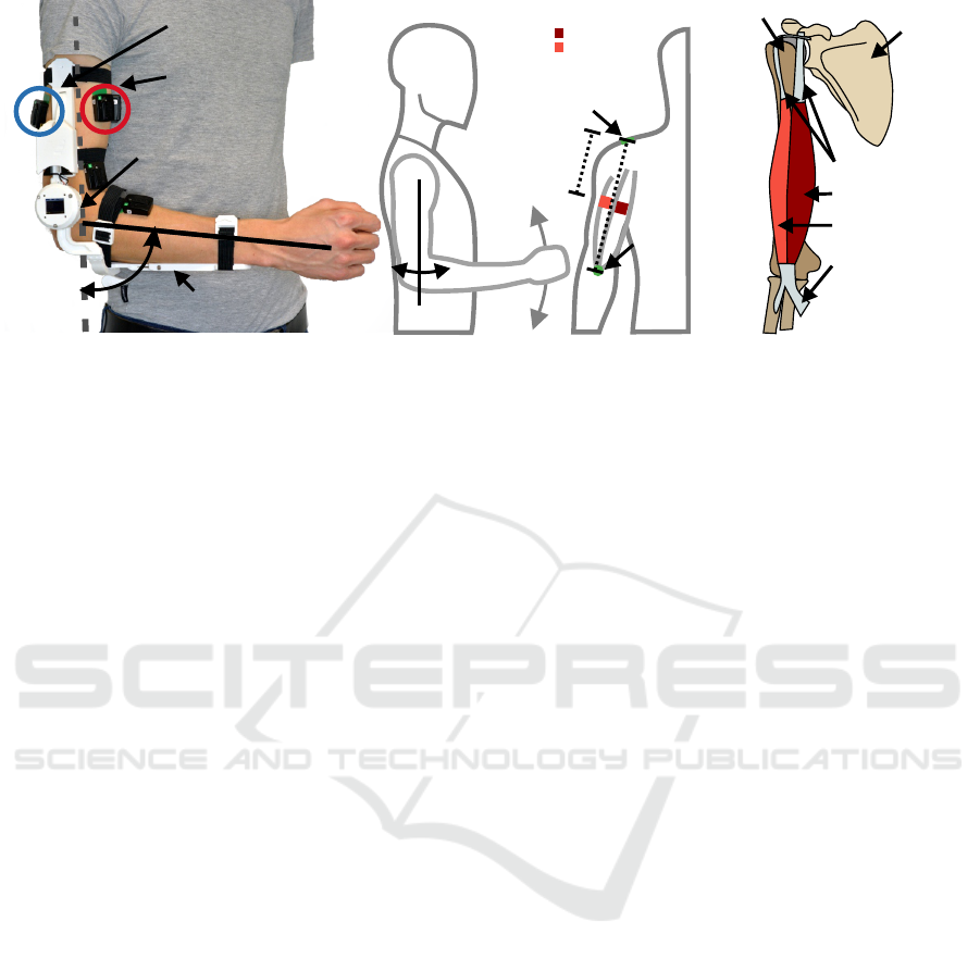
Figure 1: (a) shows the measurement orthosis on the elbow using ﬂexible straps, allowing for adaptation to different subjects.

The sEMG sensors were placed on the short and long head of the biceps and long and lateral head of the triceps, with the

wrist rotation in a neutral position. The lower experimental posture is shown in (A) and (B), with the angle of the upper arm

(α) being zero (long axis of the upper arm is pointing towards the ground). In (C) the right arm is shown in the coronal plane

from an anterior perspective, with the color code of red indicating the biceps sensors. The distance from the acromion to the

innervation zone is also noted. (D) shows a schematic depiction of the long and the short head of the biceps brachii. The right

shoulder is shown from the anterior perspective. At the top the scapular is shown where the two tendons for the individual

biceps heads are attached. The long head tendon wraps around the humerus to add stability to the joint. Whereas the short

head is connected to the anterior structure of the scapular and links directly down to the muscle belly. At the distal end of the

muscle belly, both heads merge into a common tendon. (A), (B), and (C) were adopted and modiﬁed from (Grimmelsmann

et al., 2023). (D) was modiﬁed based on (Sch

unke et al., 2010).

To be able to evaluate the size of the error, the

test prediction is compared to a baseline. To obtain a

baseline, the regression output is set to the regression

input.

2.4 Setup 2: Leave-One-out, Subject as

Variable

In the second setup, the regression is done with (I)

a linear regression with only the activation as input,

(II) a linear regression with activation, elbow angle,

elbow angular velocity, the weight of the dumbbell,

and the angle of the upper arm, and (III) a FFN

with the rectiﬁed linear unit as activation function

and the same ﬁve inputs as (II). The motivation for

these three different conﬁgurations was a granular

extension of the architecture. The elbow angle is

chosen as an input caused by the different utilisation

of the muscles over the elbow angle (Chang et al.,

1999). One property of the muscle ﬁbre itself is

the velocity-dependent force generation. This is why

the elbow velocity is taken as an input. The two

biceps heads attach via their respective tendons to

different locations on the shoulder (Sch

unke et al.,

2010). Therefore, the angle of the upper arm has

potentially an impact on the activation for the short

head of the biceps. The long head of the biceps needs

to stabilise the shoulder more with additional weight

in the hand.

The train/ test split strategy is different from setup

1. Here, the training is performed on all experiments

from all subjects excluding all experiments of one

subject. This excluded subject is used as the test

data set. This training/ test split is done ones for the

direction long head to short head and ones for the

other direction. As a result, 31 · 2 training and test

sets are created.

The input activation is scaled for each subject with

a standard scaler. The elbow angle (θ), the elbow

angular velocity (ω), the weight of the dumbbell, and

the angle of the upper arm (α) are scaled combined

over all subjects again with a standard scaler.

Before training, the activation is ﬁltered with a

symmetrical rolling mean. The whole training of

setup 2 was optimised using the adam algorithm

(Kingma and Ba, 2015) with a learning rate of 0.001

and the MAE as loss function.

2.5 Validation of the Virtual Sensor via

a Domain Knowledge Based Model

The model shown in ﬁg. 2 was also used for validation

of the virtual sensor but with one input channel

(biceps) disabled. The remaining biceps channel was

fed into the model at the point where the neural

activation was computed as described in ﬁg. 3(B,C).

Predicting the Level of Co-Activation of One Muscle Head from the Other Muscle Head of the Biceps Brachii Muscle by Linear Regression

and Shallow Feedforward Neural Networks

615

contraction dynamics

muscle

force

passive elast.force-l.

force-v.

max

muscle

activation

muscle length

muscle velocity

contraction dynamics

muscle

force

passive elast.force-l.

force-v.

max

muscle

activation

muscle length

muscle velocity

muscle

activation

muscle

activation

neural act.

A-model

neural

activation

neural act.

A-model

muscle act.

neural

activation

muscle act.

upper arm angle α

activation dyn.

activation level

time

u = f(e,u,u)

u(t)

e(t)

activation dyn.

joint geometry

elbow

eqns. of motion

CoG

elbow

neural sig.

sEMG & angle

muscle 1

muscle 2

activation level

time

u = f(e,u,u)

u(t)

e(t)

preprocessing

activation level

preprocessing

|abs|

Butterworth

|abs|

Butterworth

activation level

time

u = f(e,u,u)

u(t)

e(t)

joint geometry

elbow

EMG

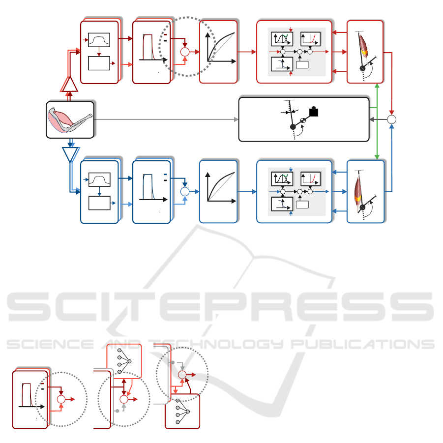
Figure 2: Depiction of the signal ﬂow of the biomechanical model. The biomechanical model which is used to calculate the

neuronal activation and to validate the virtual sensor is shown. The signal chart starts on the left with the four sEMG channels.

The two biceps channels are shown in two shades of red at the top of the arm box. The triceps is shown in two shades of

blue at the bottom. The sEMG signals are ampliﬁed and fed into a preprocessing submodel. The next submodel calculates

the neuronal activation for each of the muscle heads. One of these activations is used as an input for the regression. The other

activation is used as the target for the regression. In the biomechanical model, the activation is fed into the next submodels

until the torque of the biceps and the triceps sum up to a superimposed torque. This torque is used with dynamics equations to

calculate the angle of the elbow. This angle is in the validation step compared to the measured angle. The dotted, grey circle

marks the spot where in ﬁg. 3 different structures replace the original structure (Grimmelsmann et al., 2023).

activation level

time

u = f(e,u,u)

u(t)

e(t)

activation level

time

u = f(e,u,u)

u(t)

e(t)

(A) (B) (C)

virtual sensor

Figure 3: (a) original structure of how neural activation of

two heads was added as shown in ﬁg. 2 (cmp. dotted, grey

circle). (B) and (C) are the possible replacements for ﬁgure

(A). (A) uses both neuronal activations from the activation

dynamics. (B) shows the structure when using a virtual

sensor for the long head of the biceps. In (C) the structure is

shown for a virtual sensor for the short head of the biceps.

This activation was fed into the pre-trained virtual

sensor from section 2.4 to get the replacement channel

for the disabled one. The performance of the

virtual sensor was then measured by comparing the

simulated elbow angle θ with the measured elbow

angle θ

meas

. As introduced in (Grimmelsmann

et al., 2023), the quality score (QS) was used as

a performance indicator. The indicator QS allows

for comparison between different lengths, ranges and

shapes of a limb movement. A quality score QS of

zero means that no voluntary movement is visible,

whereas a QS=1 represents an optimal movement

prediction.

Two different conﬁgurations can be compared

with the baseline. The baseline is the simulation

where none of the two biceps channels are disabled.

Here, all available measured information is used.

In the ﬁrst conﬁguration, the sEMG of the long

head was disabled and the activation of this head

was provided via the virtual sensor (trained on the

direction from short head to long head). In the second

conﬁguration, the short head was disabled and the

activation was provided via the virtual sensor (trained

on the direction long head to the short head).

2.6 sEMG Post Measurement

Assessment

The sEMG post measurement assessment was done

via the virtual sensor from setup 2 (section 2.4).

The goal was to use the general training (on all

subject but one) in comparison to the speciﬁc test

BIOSIGNALS 2024 - 17th International Conference on Bio-inspired Systems and Signal Processing

616

(only one subject). This is based on the assumption

that both biceps heads co-contract as a result of the

shared distal tendon. The test prediction from setup

2 was used and plotted to the measured activation.

The results are shown in section 3.4 and evaluated

manually. This method can be used to provide an idea

of the signal quality to an experimenter after or during

the sEMG measurement.

3 RESULTS

The result section mirrors the structure of the methods

section. First, the results for the regression on

individual experiments are shown. After that, the

results from the leave-one-out strategy are described.

The next part is the validation of the trained sensors

by using it in a biomechanical model of the human

elbow joint. In the end of the result section

the possibility of the sEMG assessment using the

introduced method is shown.

3.1 Regression on Individual

Experiment Varies Between

Subjects

The 246 training MAE and the 246 test MAE of setup

1 show a maximal absolute difference of 0.012. The

test errors are sorted in two different ways.

First, they are sorted by the four experiments as

shown in ﬁg. 4. The variation between experimental

conditions is not signiﬁcant. Second, the training and

test errors are sorted by the subjects. This results in

31 distributions as shown in ﬁg. 5. The individual

distributions show greater variations in MAE, in the

Figure 4: The ﬁgure shows the distribution of the MAE

over the experiment type in a box and whisker plot. The

box marks the interquartile range (IQR), and the whiskers

represent data of 1.5· IQR. The MAE for the test set is

shown. All four experiments results in similar distributions.

mean as well as also in the range of the distribution.

One reason for this is the lower number of data points

within each distribution. Compared to the baseline,

the performance is only better for some subjects. The

subject with the id 28 has a lower MAE compared

to the baseline. In contrast to the subject with the id

26 which shows similar MAE values. Some of the

subjects (e.g. subject id 26) have signiﬁcantly lower

MAE compared to others. The resulting mean of the

MAE for the baseline is equal to mean of the MAE

for the virtual sensor (Baseline MAE=0.601, setup 1:

virt. short MAE=0.538, virt. long MAE=0.546)

3.2 Small Extension in the Architecture

Makes Interpretation Possible

The results for setup 2 are more diverse. The training

was performed with all but one subject to obtain a

general model, which could then be tested with the

left-out subject. The setup contains three different

conﬁgurations. Conﬁguration (I) is a linear regression

with only the activation as input. Conﬁguration (II)

is a linear regression with activation, elbow angle,

elbow angular velocity, weight of the dumbbell, and

the angle of the upper arm. Finally, conﬁguration (III)

is a feed-forward net with rectiﬁed linear unit as an

activation function and the same ﬁve inputs as for (II).

The ﬁrst conﬁguration is a model comparable

to the model from setup 1. However, the trained

virtual sensor should generalise over more subjects

and experiments than in setup 1. The results are

shown in ﬁg. 6.

Comparing setup 2 conﬁguration (I) with the

baseline shows some performance improvement

(baseline MAE=0.601, setup 2 (I): test virt. short

MAE=0.476, test virt. long: MAE=0.480, training

virt. short: 0.479, training virt. MAE=long: 0.484).

In conﬁguration (II), the input dimension is

expanded to ﬁve. The additional information leads

to larger differences between the two directions for

some subjects (e.g. subject ids [32,40]).

The expansion of the input dimension leads to

similar MAEs (baseline MAE=0.601, setup 2 (I): test

virt. short MAE=0.468, test virt. long: MAE=0.482,

training virt. short: 0.465, training virt. MAE=long:

0.481).

The last expansion step in the conﬁguration is to

add non-linearity via an activation function (rectiﬁed

linear unit). The results of this conﬁguration (III)

match the trend shown for conﬁgurations (I) and

(II). The distinction between the two directions is

clearer with this extension. The overall training

MAE and test MAE are lower than in the previous

conﬁgurations (baseline MAE=0.601, setup 2 (I) test

Predicting the Level of Co-Activation of One Muscle Head from the Other Muscle Head of the Biceps Brachii Muscle by Linear Regression

and Shallow Feedforward Neural Networks

617

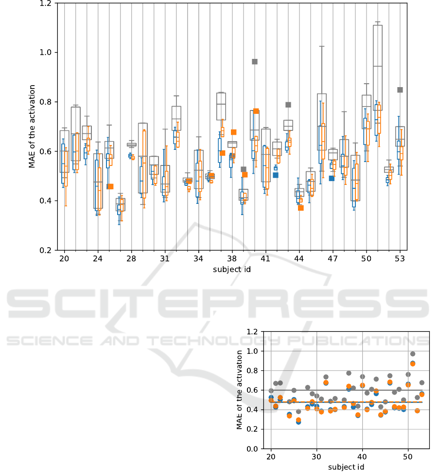
Figure 5: Box and whisker plot of the MAE over the subject id. The general structure is the same as in ﬁg. 4. There are outliers

in these distributions marked by boxes. The color represents the direction of the regression. Blue shows the distribution from

the virtual sensor for the short head. Orange shows the virtual sensor for the long head. Overall more variation of the median

and the IQR is present in this plot. The corresponding data for the training is shown in grey.

virt. short MAE=0.405, test virt. long: MAE=0.367,

training virt. short: 0.372, training virt. MAE=long:

0.347).

3.3 The Virtual Sensor Is Viable for

Using It in a Biomechanical Model

for Movement Prediction

To validate the previously trained virtual sensor, the

sensor is used as a replacement input channel in the

biomechanical model. For that, the virtual sensor

trained with the leave-one-subject-out-strategy and

conﬁguration (III) is used. In contrast to the results

before, the loss function is replaced by the quality

score (QS) between the measured elbow angle and

the predicted elbow angle. A higher value means

a better result. The data shown in ﬁg. 9 uses

the two directions (from long head to short head

and vice versa) and the baseline prediction of the

biomechanical model. Some variations between these

three results are visible for individual subjects. In

general, two main trends can be identiﬁed. The

direction long head to short head tend to increase the

prediction performance of the biomechanical model

Figure 6: MAE plotted over subject id. The different colors

represent the training MAE (grey) and the test MAE for the

different directions (from short to long head = orange and

vice versa = blue). The lines indicate the mean of the error

over all subjects. The subject dependence is similar to the

dependence shown in ﬁg. 5. Minor differences between the

two directions can be seen for some subjects.

slightly. Using the other direction the biomechanical

model shows similar results as with the baseline (both

sEMG channels used). The respective values are:

baseline: QS=0.324, virt. short: QS=0.346, virt.

long: QS=0.324.

BIOSIGNALS 2024 - 17th International Conference on Bio-inspired Systems and Signal Processing

618

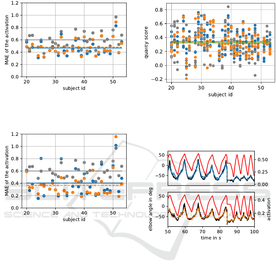
Figure 7: The structure of the ﬁgure is the same as ﬁg. 6.

The only difference is the underlying data. The overall

training MAE and test MAE are similar to conﬁguration (I).

The training MAE is slightly lower than the test MAE which

indicates a small overﬁtting.

Figure 8: Same structure as ﬁgure ﬁg. 6. Conﬁguration

(III) is used for the underlying data. This increase in

model complexity leads to a better distinction between

the directions (from short to long head = orange and vice

versa = blue). The training MAE is shown in grey. The

lines indicate the mean of the error over all subjects.

The loss is generally lower as compared to the other two

conﬁgurations.

3.4 Virtual Sensor Compared to

Measured Signal Can Serve as

sEMG Assessment

A deeper analysis of the results from the virtual sensor

with conﬁguration (III) allows for an assessment

of the sEMG. Therefore, the outputs of the two

virtual sensors for the two respective directions were

compared. Two exemplary results are chosen from

different subjects. Figure 10 shows one of the subjects

for which the virtual sensor performed well. The

two virtually created activations of this subject are in

phase with each other and with the elbow angle.

In contrast to that, the course of the activation

Figure 9: Prediction performance of the biomechanical

model utilising: both measured sEMG channel (grey),

measured sEMG from the long head plus the virtual sensor

for the short head (blue), measured sEMG from the short

head plus the virtual sensor for the long head (orange). The

subject id is shown vs. the quality score. The mean score is

shown as a line over all subject ids.

Figure 10: Time series of the two virtual sensors for subject

id 24 and the two activations from the measured sEMG.

In the upper panel both signals for the short head are

shown. The lower panel shows the signals for the long

head. The blue line represents the virtual sensor for the

virtual long head. In orange the virtual sensor for the short

head is shown. As a reference, the angle of the elbow is

plotted in red and the activation derived from the measured

sEMG plotted in black. The different experiments were

concatenated. The discontinuity at time 83 s is the change

of the experiment.

from the virutal sensor for the two directions can

be different for a subject. One of these subjects is

shown on ﬁg. 11. Comparing the two virtually created

activations for these subjects shows a discrepancy in

the phases.

The discrepancy is also present across all

experiments. With this plot, the used sEMG can be

manually assessed.

Predicting the Level of Co-Activation of One Muscle Head from the Other Muscle Head of the Biceps Brachii Muscle by Linear Regression

and Shallow Feedforward Neural Networks

619

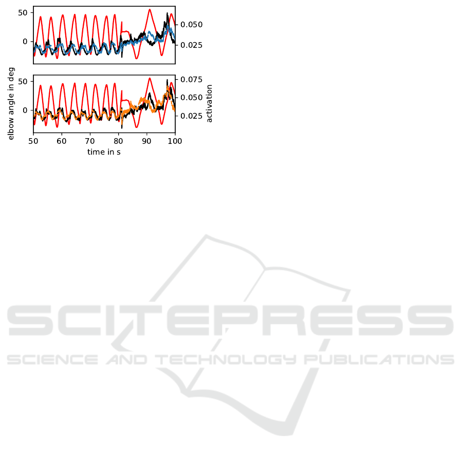
Figure 11: (Cmp. to ﬁg. 10) Time series of the two virtual

sensors and the two activation derived from the measured

sEMG of subject id 32. The color code is consistent

with ﬁg. 10. Here, the experiments changes at time 81s.

The activation from the measured short head (black, lower

panel) is slightly out of phase. Whereas the activation from

the measured long head (black, upper panel) has a higher

phase angle. The corresponding virtual sensor shows the

same phase. By comparing the measure (black) with the

virtual course (blue), the discrepancy is visible.

4 DISCUSSION

In this work, different architectures and training

strategies for the regression of two muscle heads

are presented. The architecture is expanded from

a linear regression with one input to a shallow ffn

with ﬁve inputs. The presented strategies started with

the training based on the individual experiments and

ended with the training on all but one subject.

As a result of the regression, virtual sensors are

obtained that are suitable as a replacement input to a

biomechanical model for limb movement prediction.

The underlying architecture of the virtual sensor

contains linear regression and shallow FFN. The

results of the linear regression ﬁt the general

hypothesis that the two biceps heads are usually co-

activated in the described experimental paradigm.

Using an architecture with more degrees of

freedom, it is possible to differentiate between the

two muscle heads. This will be crucial when

creating a virtual sensor for a different muscle (like

the brachialis). Additionally, the virtual sensors

generated via leave-one-out learning allow for basic

sEMG assessment.

A slight overﬁtting in the leave-one-out strategy

with the conﬁguration (III) is visible. The manual

inspection of each test set conﬁrms comparable

performance between the training and the test set.

One reason for the overﬁtting could be the relatively

high sample frequency of 1.1kHz.

The results of this study can be used as a simple

sEMG assessment tool for data centric AI approaches.

The shallow structure of the used FFN allows other

researchers to train a similar model for their own data.

Furthermore, the results lay the foundation to

push the boundaries of sEMG measurement as a next

step. The general problem of measuring deep muscles

with sEMG (such as the brachialis) may be partially

solved by extending the presented method via other

architectures beside FFN. In this use case, the virtual

sensor will be learned from muscle to muscle to

provide a signal of an unknown muscle head for a

biomechanical model. A potential time dependency

between different muscles activations could require

model with a RNN or LSTM architecture.

ACKNOWLEDGEMENTS

This work has been supported by the research training

group “Dataninja” (Trustworthy AI for Seamless

Problem Solving: Next Generation Intelligence Joins

Robust Data Analysis) and by the “TransCareTech”

project (Transformation in Care & Technology), both

funded by the German federal state of North Rhine-

Westfalia.

We would like to thank Philipp J

unemann and

Irina L

owen for their valuable contributions during

proofreading.

REFERENCES

Chang, Y.-W., Su, F.-C., Wu, H.-W., and An, K.-N. (1999).

Optimum length of muscle contraction. Clinical

Biomechanics, 14(8):537–542.

del Toro, S. F., Wei, Y., Olmeda, E., Ren, L., Guowu,

W., and D

ıaz, V. (2019). Validation of a low-cost

electromyography (EMG) system via a commercial

and accurate EMG device: Pilot study. Sensors,

19(23):5214.

Grimmelsmann, N., Mechtenberg, M., Schenck, W.,

Meyer, H. G., and Schneider, A. (2023). sEMG-

based prediction of human forearm movements

utilizing a biomechanical model based on individual

anatomical/ physiological measures and a reduced set

of optimization parameters. PLOS ONE, 18(8):1–28.

Hill, A. V. (1964). The effect of load on the heat of

shortening of muscle. Proceedings of the Royal

Society of London. Series B. Biological Sciences.

Publisher: The Royal Society London.

Kim, M., Chung, W. K., and Kim, K. (2019). Preliminary

Study of Virtual sEMG Signal-Assisted Classiﬁcation.

In 2019 IEEE 16th International Conference on

Rehabilitation Robotics (ICORR), pages 1133–1138.

BIOSIGNALS 2024 - 17th International Conference on Bio-inspired Systems and Signal Processing

620

Kingma, D. and Ba, J. (2015). Adam: A method for

stochastic optimization. In International Conference

on Learning Representations (ICLR), San Diega, CA,

USA.

Koo, T. K. and Mak, A. F. (2005). Feasibility of using emg

driven neuromusculoskeletal model for prediction

of dynamic movement of the elbow. Journal of

Electromyography and Kinesiology, 15(1):12–26.

Leserri, D., Grimmelsmann, N., Mechtenberg, M., Meyer,

H. G., and Schneider, A. (2022). Evaluation of

semg signal features and segmentation parameters for

limb movement prediction using a feedforward neural

network. Mathematics, 10(6).

Machado, J. C., Cene, V. H., and Balbinot, A. (2019).

Recurrent Neural Network as Estimator for a Virtual

sEMG Channel. In 2019 41st Annual International

Conference of the IEEE Engineering in Medicine and

Biology Society (EMBC), pages 3620–3623. IEEE.

Mechtenberg, M., Grimmelsmann, N., Meyer, H. G., and

Schneider, A. (2023). Surface electromyographic

recordings of the biceps and triceps brachii for various

postures, motion velocities and load conditions. FH

Bielefeld.

Merletti, R. and Farina, D. (2008). Analysis of

intramuscular electromyogram signals. Philosophical

Transactions of the Royal Society A: Mathematical,

Physical and Engineering Sciences, 367(1887):357–

368.

Merletti, R., Farina, D., and Holobar, A. (2018). Surface

Electromyography (sEMG), pages 1–22. John Wiley

& Sons, Ltd.

Pedregosa, F., Varoquaux, G., Gramfort, A., Michel, V.,

Thirion, B., Grisel, O., Blondel, M., Prettenhofer,

P., Weiss, R., Dubourg, V., Vanderplas, J., Passos,

A., Cournapeau, D., Brucher, M., Perrot, M., and

Duchesnay, E. (2011). Scikit-learn: Machine learning

in Python. Journal of Machine Learning Research,

12:2825–2830.

Sch

unke, M., Schulte, E., Schumacher, U., Voll, M., and

Sch

unke, M. (2010). Thieme atlas of anatomy:

general anatomy and musculoskeletal system; 100

tables. Thieme, corr. repr., plus version edition.

Zajac, F. E. (1989). Muscle and tendon: properties, models,

scaling, and application to biomechanics and motor

control. Crit Rev Biomed Eng, 17(4):359–411.

Predicting the Level of Co-Activation of One Muscle Head from the Other Muscle Head of the Biceps Brachii Muscle by Linear Regression

and Shallow Feedforward Neural Networks

621