Training Methods for Regularizing Gradients on Multi-Task Image
Restoration Problems
∗
Samuel Willingham
1,2 a
, M
˚
arten Sj
¨
ostr
¨
om
2 b
and Christine Guillemot
1 c
1
Inria Rennes, Rennes, France
2
Mid Sweden University, Sundsvall, Sweden
Keywords:
Inverse Problems, Computer Vision, Image Restoration, Deep Equilibrium Models, Deep Priors.
Abstract:
Inverse problems refer to the task of reconstructing a clean signal from a degraded observation. In imaging,
this pertains to restoration problems like denoising, super-resolution or in-painting. Because inverse problems
are often ill-posed, regularization based on prior information is needed. Plug-and-play (pnp) approaches take
a general approach to regularization and plug a deep denoiser into an iterative solver for inverse problems.
However, considering the inverse problems at hand in training could improve reconstruction performance at
test-time. Deep equilibrium models allow for the training of multi-task priors on the reconstruction error via
an estimate of the iterative method’s fixed-point (FP). This paper investigates the intersection of pnp and DEQ
models for the training of a regularizing gradient (RG) and derives an upper bound for the reconstruction loss
of a gradient-descent (GD) procedure. Based on this upper bound, two procedures for the training of RGs
are proposed and compared: One optimizes the upper bound directly, the other trains a deep equilibrium GD
(DEQGD) procedure and uses the bound for regularization. The resulting regularized RG (RERG) produces
consistently good reconstructions across different inverse problems, while the other RGs tend to have some
inverse problems on which they provide inferior reconstructions.
1 INTRODUCTION
This paper considers image enhancement and restora-
tion through the lens of inverse problems. Inverse
problems refer to a large subset of signal processing
applications, where one attempts to recover a signal
from a flawed or noisy observation. In imaging, this
refers to the reconstruction of degraded images - e.g.
images with missing pixels, or low-resolution images.
Because inverse problems can be ill-posed, some kind
of regularization that imposes prior assumptions on
the search-space is necessary.
One approach to solving the regularization prob-
lem for inverse problems are the pnp methods
(Venkatakrishnan et al., 2013; Pesquet et al., 2021;
Chan et al., 2016; Le Pendu and Guillemot, 2023;
Zhang et al., 2021). These methods use pre-trained
a
https://orcid.org/0009-0005-1954-1143
b
https://orcid.org/0000-0003-3751-6089
c
https://orcid.org/0000-0003-1604-967X
∗
This project has received funding from the European
Union’s Horizon 2020 research and innovation programme
under the Marie Skłodowska-Curie grant agreement No
956770.
priors in iterative algorithms like the alternating di-
rection method of multipliers (ADMM) (Chan et al.,
2016), the forward-backward algorithm (FB) (Pes-
quet et al., 2021), or GD. ADMM and FB use a reg-
ularizing proximal operator (PO) that represents the
prior. This PO can be replaced with a deep Gaussian
denoiser (Venkatakrishnan et al., 2013; Chan et al.,
2016), leading to good reconstruction performance.
Apart from methods based on POs, there are other
approaches like regularization by denoising (Romano
et al., 2017), or the pnp Regularizing Gradient (pn-
pReG) (Fermanian et al., 2023), which trains a RG
that is used to regularize a pnp GD procedure. Over-
all, pnp approaches are very general in application,
but because they are not trained on the inverse prob-
lems at hand, performance can be further improved
(Willingham et al., 2023).
To train a full iterative scheme directly on the in-
verse problem at hand, deep equilibrium (DEQ) mod-
els (Gilton et al., 2021; Bai et al., 2019; Fung et al.,
2022; Winston and Kolter, 2020; Ling et al., 2022)
can be used to train an entire iterative method via its
FP. This can be done in a Jacobian-free manner (Fung
et al., 2022), which is effectively one step of back-
Willingham, S., Sjöström, M. and Guillemot, C.
Training Methods for Regularizing Gradients on Multi-Task Image Restoration Problems.
DOI: 10.5220/0012368100003660
Paper published under CC license (CC BY-NC-ND 4.0)
In Proceedings of the 19th International Joint Conference on Computer Vision, Imaging and Computer Graphics Theory and Applications (VISIGRAPP 2024) - Volume 3: VISAPP, pages
145-153
ISBN: 978-989-758-679-8; ISSN: 2184-4321
Proceedings Copyright © 2024 by SCITEPRESS – Science and Technology Publications, Lda.
145

propagation on the iterative method, starting at the FP.
When applied to a range of inverse problems, multi-
task (MT) DEQ models (Willingham et al., 2023) al-
low for the training of MT priors on a large range of
inverse problems by leveraging the reconstruction er-
ror over a range of inverse problems, leading to strong
MT reconstruction performance.
However, DEQ models heavily depend on finding
a good approximation of the FP. This can be quite dif-
ficult, as convergence is not always guaranteed and
even if the algorithm does converge, this can take a
large amount of iterations or lead to bad estimates of
the FP. As a result, this can lead to sub-optimal pa-
rameter updates.
The contributions of this paper are:
• This paper investigates and compares different ap-
proaches of training a RG for a range of inverse
problems.
• We show that the difference between the GD
and the FB reconstruction errors is bounded from
above. This upper bound led us to propose a
method for training the RG using a FB optimiza-
tion method. The resulting RG is called RG1.
• We also propose a procedure that uses the up-
per bound to regularize the training of a multi-
task DEQGD procedure. This regularized RG
(RERG) leads to strong reconstruction perfor-
mance on a range of inverse problems by taking
into account the FB and the GD reconstruction-
errors. In testing, RERG displayed performance
close to whichever was better (RG1 or DEQGD)
on any given inverse problem.
• We compare four different RGs on a range of in-
verse problems and discuss the differences.
2 RELATED WORKS AND
THEORY
2.1 Inverse Problems and Maximum a
Posteriori Estimation
We consider the image formation model
y
y
y = A
ˆ
x
x
x + ε
ε
ε, (1)
where y
y
y denotes the degraded observation,
ˆ
x
x
x ∈ R
d
is
the ground truth image, A : R
d
→ R
d
′
denotes the
degradation operation and ε
ε
ε ∈ R
d
′
denotes additive
white Gaussian noise (AWGN) with standard devia-
tion σ ≥ 0, and d,d
′
∈ N.
In this paper, we consider maximum a posteri-
ori (MAP) estimation (Venkatakrishnan et al., 2013;
Zhang et al., 2021; Le Pendu and Guillemot, 2023;
Fermanian et al., 2023), meaning the search for an
x
x
x ∈ R
d
, that maximizes p(x
x
x | y
y
y); i.e. the x
x
x that is the
most likely to have caused observation y
y
y. Assuming
uniqueness, this leads to
ˆ
x
x
x
MAP
= argmax
x
x
x
p(x
x
x | y
y
y) (2)
= argmin
x
x
x
−log p(y
y
y | x
x
x) − log p(x
x
x) (3)
= argmin
x
x
x
1
2
∥Ax
x
x − y
y
y∥
2
2
+ σ
2
R(x
x
x), (4)
where we set R(x
x
x) := −log p(x
x
x) and ∥·∥
2
denotes the
2-norm. The expression with the norm is called the
data-term. R is called the regularizer and represents
the prior distribution.
The MAP estimation problem can be solved us-
ing iterative algorithms, like the ADMM, FB or GD
algorithm.
2.2 Plug-and-Play Regularizing
Gradient
PnpReG (Fermanian et al., 2023) deals with the regu-
larization problem in equation (4) by linking the gra-
dient of the regularizer with its proximal operator
prox
σ
2
R
(z
z
z) := argmin
x
x
x
1
2
∥x
x
x − z
z
z∥
2
2
+ σ
2
R(x
x
x). (5)
As shown in (Fermanian et al., 2023), it holds that for
all z
z
z ∈ R
d
and σ ≥ 0
σ
2
δR(x
x
x)
δx
x
x



x
x
x=prox
σ
2
R
(z
z
z)
= z
z
z − prox
σ
2
R
(z
z
z). (6)
Thus, the loss
L
link
σ
(z
z
z) = ∥σ
2
G(P
σ
2
(z
z
z)) − (z
z
z − P
σ
2
(z
z
z))∥
2
2
(7)
is used to train the gradient G of the regularizer corre-
sponding to the PO defined by a Gaussian denoiser.
This uses the approximation P
σ
2
(x
x
x) ≈ prox
σ
2
R
(z
z
z),
where P
σ
2
(x
x
x) is trained as a deep-denoiser. The over-
all training loss is
L
pnpReG
= δ∥P
σ
2
(
˜
z
z
z) −
ˆ
x
x
x∥
1
+ λL
link
σ
(
˜
z
z
z), (8)
where ∥·∥
1
is the L1 norm, λ > 0,
˜
z
z
z =
ˆ
x
x
x+ε
ε
ε, with ε
ε
ε be-
ing AWGN with standard deviation σ
0
> 0. Further-
more, δ is equal to 1 if σ = σ
0
and δ is equal to zero,
otherwise. This leads to a RG that is trained jointly
with a denoiser and produces strong reconstruction re-
sults when used as regularization in a GD algorithm.
Pnp approaches, however, do not take the reconstruc-
tion error into account and could potentially be im-
proved by considering the inverse problems at hand.
VISAPP 2024 - 19th International Conference on Computer Vision Theory and Applications
146

2.3 Deep Equilibrium Models
DEQ models (Gilton et al., 2021; Bai et al., 2019;
Fung et al., 2022; Winston and Kolter, 2020; Ling
et al., 2022) allow for the training of a whole iterative
procedure h
θ
via the corresponding FP x
x
x
h
and the re-
sulting reconstruction error. In (Bai et al., 2019), this
is done by considering h
θ
(x
x
x
h
) = x
x
x
h
and thus
δx
x
x
h
δθ
=
δh
θ
(x
x
x)
δx
x
x





x
x
x=x
x
x
h
δx
x
x
h
δθ
+
δh
θ
(x
x
x)
δθ





x
x
x=x
x
x
h
. (9)
Rearranging this and plugging δ x
x
x
h
/δθ into the
derivative of loss l : R
d
× R
d
→ R with respect to θ,
yields
δl(
ˆ
x
x
x,x
x
x
h
)
δθ
=
δl(
ˆ
x
x
x,x
x
x)
δx
x
x





x
x
x=x
x
x
h
δx
x
x
h
δθ
(10)
=
δl(
ˆ
x
x
x,x
x
x)
δx
x
x





x
x
x=x
x
x
h
J
−1
δh
θ
(x
x
x)
δθ





x
x
x=x
x
x
h
, (11)
where the Jacobian J := id −
δh
θ
(x
x
x)
δx
x
x



x
x
x=x
x
x
h
exists and is
invertible (Fung et al., 2022). Assuming the inverse
of J to be equal to the identity still yields a direction
of descent (Fung et al., 2022). This is called Jacobian-
free back-propagation and can be likened to a single
step of traditional back-propagation, using the FP x
x
x
h
as input.
The following section will introduce important
definitions that we shall use to expand existing the-
ory and propose different training methods for RGs.
3 DEFINITIONS
As it is our intent to train and compare RGs to be used
in a GD algorithm, we shall first define the necessary
functions and expressions.
We define the two iterative algorithms to solve the
MAP estimation problem in 4. One is the FB algo-
rithm (Pesquet et al., 2021) that was also used for the
multi-task DEQ (MTDEQ) prior (Willingham et al.,
2023), where for each ground truth image
ˆ
x
x
x, we pick
a degradation A : R
d
→ R
d
′
and noise-level σ at ran-
dom, generating noise ε
ε
ε, leading to a degraded obser-
vation y
y
y = A(
ˆ
x
x
x) + ε
ε
ε. For z
z
z ∈ R
d
. One iteration of the
FB algorithm takes the form
f
σ,A,θ
(z
z
z,y
y
y) := P
θ,ησ
2
(z
z
z − ηD(z
z
z,y
y
y)), (12)
where P
θ,σ
2
is a regularizer in form of a DRUNet (as
in (Le Pendu and Guillemot, 2023) and (Zhang et al.,
2021)) with parameters θ used on noise-level σ ≥ 0
with step-size η ∈ R. For z
z
z ∈ R
d
, we define
D(z
z
z,y
y
y) :=
δ
1
2
∥Ax
x
x − y
y
y∥
2
2
δx
x
x



x
x
x=z
z
z
(13)
as the derivative of the data-term.
Similarly, for z
z
z ∈ R
d
, one iteration of the gradient-
descent algorithm is defined as
g
σ,A,θ
(z
z
z,y
y
y) := z
z
z − η

D(z
z
z,y
y
y) + σ
2
G
θ
(z
z
z,y
y
y)

, (14)
where G
θ
is the network representing the gradient of
the regularizer in (4), which we also refer to as RG.
We use the same 3-channel DRU-net architecture that
is used in (Fermanian et al., 2023). x
x
x
g,σ,A,θ
(y
y
y) and
x
x
x
f ,σ,A,θ
(y
y
y) are the FPs of g
σ,A,θ
(·,y
y
y) and f
σ,A,θ
(·,y
y
y),
respectively. For clarity of notation, the indices σ,A
and θ as well as the argument y
y
y will be omitted, when
this is allowed by the context.
For ease of notation, we define the reconstruction
errors
L
FB
σ,A,θ
:= ∥ f (x
x
x
f
) −
ˆ
x
x
x∥
2
2
(15)
L
GD
σ,A,θ
:= ∥g(x
x
x
g
) −
ˆ
x
x
x∥
2
2
(16)
where L
FB
denotes the reconstruction error of the FB
algorithm and L
GD
is the reconstruction error of the
GD algorithm.
Remark 1. Note that it is our intention to find param-
eters θ and thus, RG G
θ
, such that L
GD
is small. This
is the entity that is evaluated when computing peak
signal-to-noise ratio (PSNR) on the reconstruction.
Definition 1 (Lipschitz continuity (Bauschke et al.,
2017)). We call a function h : R
n
→ R
n
, with n ∈ N,
L-Lipschitz continuous with relation to the metric in-
duced by ∥·∥
2
and with Lipschitz constant L ≥ 0 if
and only if for all x
x
x
1
,x
x
x
2
∈ R
n
it holds that
∥h(x
x
x
1
) − h(x
x
x
2
)∥
2
≤ L∥x
x
x
1
− x
x
x
2
∥
2
. (17)
If there exists an L < 1 that permits this condition, we
call h a contraction.
Using these definitions, the following sections
will introduce an upper bound for the GD reconstruc-
tion error, propose training approaches based on said
upper bound and compare the resulting reconstruction
performance.
4 METHOD
4.1 Derivations
This section leverages the introduced definitions from
section 3 to derive a relationship between the FB re-
construction error and the GD reconstruction error
that leads to a new approach to realizing the goal in
remark 1.
Training Methods for Regularizing Gradients on Multi-Task Image Restoration Problems
147

Theorem 1. If GD procedure g is a contraction with
relation to ∥·∥
2
(with Lipschitz constant L
g
< 1), then
there exists an
˜
x
x
x ∈ R
d
, such that
∥x
x
x
g
−
ˆ
x
x
x∥
2
≤
1
1 − L
g
q
L
link
ησ
2
(
˜
x
x
x) + ∥x
x
x
f
−
ˆ
x
x
x∥
2
. (18)
Proof. By plugging
˜
x
x
x = x
x
x
f
− ηD(x
x
x
f
) into L
link
, we
get that for all η > 0 and σ ≥ 0, it holds that
L
link
ησ
2
(
˜
x
x
x) = ∥ησ
2
G(x
x
x
f
) − (x
x
x
f
− ηD(x
x
x
f
) − x
x
x
f
)∥
2
2
(19)
= ∥ησ
2
G(x
x
x
f
) + ηD(x
x
x
f
)∥
2
2
. (20)
This leads to
∥x
x
x
f
− x
x
x
g
∥
2
=∥x
x
x
f
− η(D(x
x
x
f
) + σ
2
G(x
x
x
f
)) (21)
+ η(D(x
x
x
f
) + σ
2
G(x
x
x
f
)) − x
x
x
g
∥
2
(22)
≤∥g(x
x
x
f
) − x
x
x
g
∥
2
+
q
L
link
ησ
2
(
˜
x
x
x) (23)
≤L
g
∥x
x
x
f
− x
x
x
g
∥
2
+
q
L
link
ησ
2
(
˜
x
x
x), (24)
resulting in the statement via the triangle inequality.
Remark 2. Furthermore, because for all a,b ∈ R, it
holds that a
2
+ b
2
≥ 2ab, we get
1
2
∥x
x
x
g
−
ˆ
x
x
x∥
2
2
≤
1
(1 − L
g
)
2
L
link
ησ
2
(
˜
x
x
x) + ∥x
x
x
f
−
ˆ
x
x
x∥
2
2
, (25)
allowing us to limit the GD reconstruction error (i.e.
a RG to be used in a GD algorithm) by using the two
loss-terms on the right as training objectives.
Based on remark 2, we train a GD procedure by
training a PO and RG to minimize the bound in (25).
Remark 3. It immediately follows that for
L
bound
:=
2
(1 − L
g
)
2
L
link
ησ
2
(
˜
x
x
x) + 2∥x
x
x
f
−
ˆ
x
x
x∥
2
2
, (26)
we also get that ∥x
x
x
g
−
ˆ
x
x
x∥
2
2
is bounded by a convex
combination of itself and L
bound
, or more generally
∥x
x
x
g
−
ˆ
x
x
x∥
2
2
≤ λL
bound
+ ζ∥x
x
x
g
−
ˆ
x
x
x∥
2
2
, (27)
for all λ,ζ > 0 and with λ + ζ ≥ 1.
This allows us to constrain the hypothesis-space
for the training of a deep equilibrium regularizing gra-
dient, adding regularization for the DEQ training of a
GD algorithm, leading to the RERG, for which the
training objective will be defined in the next section.
Data: Ground truth image set D, k ∈ {1,2,3}, set
of noise-levels Σ and set of degradations A;
Result: Parameters Θ for a regularizing gradient
and the corresponding proximal operator;
for a number of epochs do
for all
ˆ
x
x
x from D do
(σ,A) ← random choice from Σ × A;
y
y
y ← A
ˆ
x
x
x + ε
ε
ε, ε
ε
ε ∼ N (0, σ);
Find FPs x
x
x
f
of f
σ,A,θ
and x
x
x
g
of g
σ,A,θ
;
Calculate L
k
corresponding to the
algorithm trained;
Update parameters θ via loss L
k
;
end
end
Algorithm 1: Training algorithm for the RGs. k = 1 leads
to RG1, k = 2 gives the DEQGD and k = 3 leads to RERG.
4.2 Algorithm
Based on the definitions in section 3 and the deriva-
tions in section 4.1, we introduce the training pipeline
described in algorithm 1. This pipeline is quite simi-
lar to the one used in (Willingham et al., 2023), with
only one inverse problem considered at each iteration
and with different training objectives. We use this al-
gorithm for the training of three different RGs, via the
training objectives
L
1
:= 0.1L
link
σ
2
(x
x
x
f
− ηD(x
x
x
f
)) + L
FB
(28)
L
2
:= L
GD
(29)
L
3
:= L
1
+ 0.1L
GD
(30)
where 0.1 is an experimentally chosen hyper-
parameter, which could likely be further optimized to
improve reconstruction performance at test time. The
weighting in L
3
could also be modified to increase the
weight of L
GD
or L
1
, respectively.
Note that for the derivative of L
link
σ
2
(x
x
x
f
− ηD(x
x
x
f
))
used for the update of the parameters in algorithm 1,
we use Jacobian-free back-propagation (Fung et al.,
2022), i.e. the assumption that the approximation
δL
link
σ
2
(x
x
x
f
− ηD(x
x
x
f
))
δθ
≈
δL
link
σ
2
(x
x
x)
δθ




x
x
x=x
x
x
f
−ηD(x
x
x
f
)
(31)
yields a direction of descent.
The use of algorithm 1 with objective L
1
is differ-
ent from pnpReG in three ways:
• We replace the denoising-loss (i.e. the first
summand in (8)) with the FB reconstruction
loss, training the PO on the resulting FB
reconstruction-error rather than a Gaussian de-
noising problem.
• The algorithm evaluates L
link
at
˜
x
x
x from Theorem
1, which depends on the equilibrium point of the
VISAPP 2024 - 19th International Conference on Computer Vision Theory and Applications
148

FB algorithm, instead of evaluating L
link
on im-
ages only perturbed by AWGN, as is done in the
pnpReG method of (Fermanian et al., 2023). If we
consider only L
link
at
˜
x
x
x from Theorem 1, it would
train a PO and RG in a way such that the resulting
FB and GD algorithms have the same FP. Looking
at equation (20), this measures how ”non-fixed”
x
x
x
f
is when put into the corresponding GD proce-
dure, since the part with L
link
is equal to zero if x
x
x
f
is a FP of the GD procedure.
• We only consider the case where the σ used for
L
link
is identical with the standard deviation of the
AWGN.
Similar to (Willingham et al., 2023), we evaluate the
neural nets at images that actually appear when it-
eratively solving the MAP estimation problem from
(4) for a given inverse problem, rather than on an as-
sumed Gaussian perturbation.
Furthermore, we can use the upper bound to regu-
larize the training of a DEQGD procedure by consid-
ering the reconstruction error of the GD procedure as
well as regularizing the RG by tying it to a PO via the
bound given in (25). This constrains the hypothesis-
space by using two loss-terms that can both be used
to approach the training objective outlined in remark
1.
The following sections will highlight how the re-
sulting methods were trained and tested in order to
compare them to pnpReG (Fermanian et al., 2023),
MTDEQ (Willingham et al., 2023) and Gaussian de-
noiser plugged into the pnp ADMM algorithm (results
from (Fermanian et al., 2023)).
5 EXPERIMENTS
Using the theory and algorithm introduced in the pre-
vious sections, this section discusses the details of
training and the experiments made to compare the
trained RGs.
For the experiments we have trained three differ-
ent RGs using the pipeline outlined in algorithm 1:
• RG1, which is the prior that uses loss L
1
i.e. di-
rectly attempts to minimize the upper bound,
• A DEQGD, which uses loss L
2
, and
• RERG, which uses loss L
3
, combining both RG1
and a DEQGD.
5.1 Step-Sizes and Degradations
We use a step-size of η
GD
= 0.05 for the GD proce-
dure, and similar to (Fermanian et al., 2023), we use
the adam optimizer (Kingma and Ba, 2014) to find
the FP of the GD procedure from (14) for training.
The FB procedure uses step-size η
FB
= 0.49, which
is taken from (Willingham et al., 2023).
We consider the following degradations in train-
ing:
• Gaussian deblurring with the level of blur σ
b
in
[0,4]
• Super-resolution with factors 1,2 and 4
• Pixel-wise completion where each pixel has a
chance of p
drop
∈ [0,0.99]. Each selection of p
drop
refers to a degradation.
Additionally, we used noise-levels sampled from a
uniform distribution on Σ := [0, 50/255]. For each it-
eration, there is a 1/3 chance of choosing deblurring,
super-resolution or pixel-wise completion. After this
choice, the degree of the degradation is sampled via a
uniform distribution on the corresponding set.
5.2 Dataset and Optimizer
The networks are optimized using the adam optimizer
(Kingma and Ba, 2014) on a training-dataset consist-
ing of the data-set from DIV2k (Agustsson and Tim-
ofte, 2017), the training-set from BSD500 (Arbelaez
et al., 2011), flick2k (Lim et al., 2017) and the Wa-
terloo Exploration Database (Ma et al., 2016). Over-
all, this data-set contains 8394 images. Each iteration
takes a batch of 16 images and crops each image at a
random location to the size of 128 by 128 pixels.
For the finding of the FP, the forward iterations of
GD or FB are terminated if one or more of the follow-
ing three conditions hold:
• The forward iteration has gone on for 500 itera-
tions.
• The absolute value of any entry of an estimate is
larger than 100.
• The mean square distance between two consecu-
tive estimates is less than 10
−7
.
The first condition is necessary because of time con-
straints; the second condition is in place to avoid
the network forgetting what has been trained previ-
ously if the iterative method starts to diverge. This
avoids unreasonably large gradients in failure-cases.
The final condition is the proper convergence condi-
tion. Choosing a smaller margin for convergence or a
higher number of maximum forward iterations tends
to lead to a more accurate FP estimation. As a re-
sult, this can be expected to lead to more accurate, but
slower, training.
In our training, the networks for the RG are ini-
tialized with the pnpReG (Fermanian et al., 2023),
Training Methods for Regularizing Gradients on Multi-Task Image Restoration Problems
149

while the networks representing the PO are initial-
ized with the MTDEQ regularizer (Willingham et al.,
2023). The networks are trained for 150 epochs, start-
ing with a step-size of 10
−5
. The step-size is reduced
by 75% every 15 epochs.
5.3 Comparisons to Other Methods
We compare our different algorithms to MTDEQ
(Willingham et al., 2023), pnp ADMM with a Gaus-
sian denoiser (called Gauss in the tables) and pn-
pReG. The PSNR values for the two latter methods
are drawn from (Fermanian et al., 2023). The com-
parisons are done on set5 (Bevilacqua et al., 2012).
Hyper-parameters used for the testing of the RGs in a
GD algorithm are taken from (Fermanian et al., 2023)
and were tuned to produce the best results for pn-
pReG, meaning they were not further optimized for
RG1, DEQGD or RERG. Note that the weight of the
regularization is given by the AWGN in the inverse
problem, but for problems with no AWGN, a weight
larger than zero was chosen to allow for regulariza-
tion.
Based on these experiments, the next section will
compare the performance of the different approaches
and discuss the results.
6 RESULTS AND DISCUSSION
To showcase the differences that appear when using
the introduced bound for RG1 and RERG, this sec-
tion will compare the performance of four different
RGs and examine differences in reconstruction per-
formance.
Training a DEQGD is difficult, as convergence of
the forward iterations is elusive and in our training
only about half the iterations converged before reach-
ing 500 iterations. This is why we used adam in for-
ward iteration as well as the stopping condition of any
entry having absolute value over 100. Training RG1
was quite stable and did not lead to any larger issues
in training, as the FB algorithm used tends to be much
more stable and converge faster.
The RG1 prior performs best for completion (see
table 1), while the DEQGD performs better for many
of the other applications (especially the noisy ones).
This is likely the case because the GD procedure di-
rectly uses the (known) noise-level in each iteration.
The FB algorithm, on the other hand, uses a proxi-
mal operator, in which the link between the level of
AWGN given to the proximal operator is processed
by a neural net, necessitating a training of this rela-
tionship. For zero-noise problems with little to no
AWGN, this is a boon, because the regularization
weight in a GD procedure may become too small to
provide meaningful regularization. This is why the
weight for the regularization is chosen to be larger
than zero at test-time, when a noise-less problem is
considered.
On any given task, RERG performs close to
whichever of RG1 and DEQGD performs best, out-
performing DEQGD on most problems. This means
that using the upper bound in addition to L
GD
in train-
ing can lead to a procedure that leverages the recon-
struction errors of both, a GD and a FB algorithm to
perform well across all the degradations considered.
If one looks at the visual examples in figure 1, it ap-
pears as if the RERG avoids some of the artifacts that
appear in RG1 and DEQGD, like the blurring of the
butterfly’s pattern on the bottom right in figure 1 (b),
or the artifacts produced by RG1 in (a). While RG1
or the DEQGD both perform well for some problems
and worse for others, RERG appears to perform more
consistently across the different degradations consid-
ered.
Figure 2 shows that for inverse problems where
convergence is slow (necessitating a higher step-size)
DEQGD and RERG may converge faster, because
they are trained with a larger step-size and a limited
amount of iterations. The problem highlighted in fig-
Table 1: This table compares methods on noise-less pixel-wise completion with 80 and 90 % of the pixels missing, respec-
tively. It also displays deblurring results for σ
noise
= 0.01 and Gaussian kernels with two different levels of blur σ
b
. Results
are reported as PSNR (dB) | SSIM (Structural Similarity Index Measure (Wang et al., 2004)). Both metrics are computed on
the red green blue color channels.
Methods
Completion Deblurring
80% 90% σ
b
= 1.6 σ
b
= 2.0
Gauss 30.20 | 0.893 26.20 | 0.821 32.06 | 0.884 30.88 | 0.866
MTDEQ 30.72 | 0.897 27.09 | 0.837 32.82 | 0.898 31.83 | 0.881
pnpReG 30.36 | 0.894 26.94 | 0.830 32.51 | 0.898 31.19 | 0.884
RG1 30.58 | 0.899 27.18 | 0.837 32.31 | 0.884 31.67 | 0.877
DEQGD 29.59 | 0.892 24.34 | 0.811 32.80 | 0.901 32.03 | 0.888
RERG 30.29 | 0.894 26.86 | 0.830 32.90 | 0.902 32.17 | 0.890
VISAPP 2024 - 19th International Conference on Computer Vision Theory and Applications
150

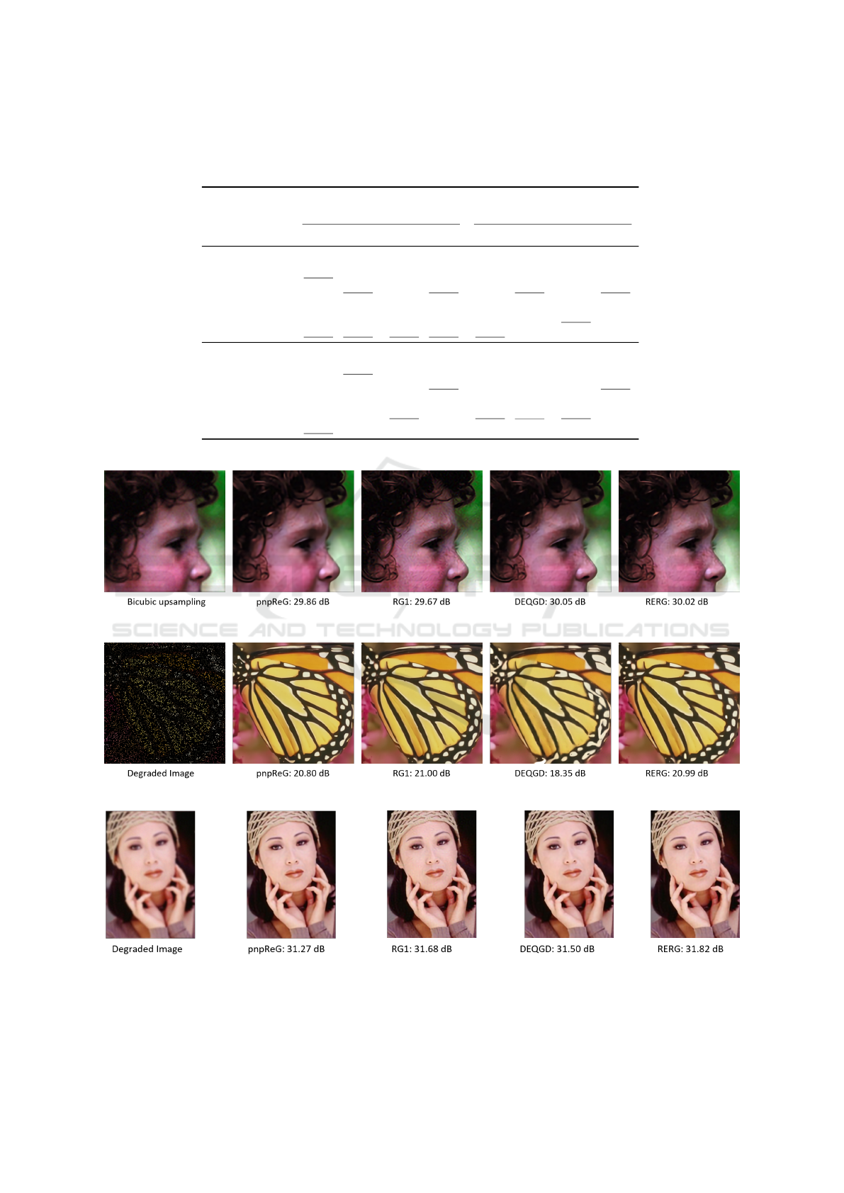
Table 2: Results for super-resolution on images that were down-sampled using a Gaussian kernel with σ
b
= 0.5 and a bicubic
kernel, respectively. This is done on a factor of 2 and 3, as well as two different noise-levels. Results are reported in the form
PSNR | SSIM.
Methods
Bicubic Gaussian
w/ σ
noise
w/ σ
noise
0.00 0.01 0.00 0.01
2x
SR
Gauss 35.20 | 0.940 33.80 | 0.917 35.14 | 0.938 32.74 | 0.900
MTDEQ 35.61 | 0.942 34.43 | 0.917 35.42 | 0.939 33.45 | 0.901
pnpReG 35.34 | 0.943 34.29 | 0.922 35.30 | 0.942 33.41 | 0.906
RG1 35.66 | 0.944 33.86 | 0.908 35.57 | 0.943 32.51 | 0.876
DEQGD 35.50 | 0.941 34.40 | 0.924 35.40 | 0.940 33.66 | 0.911
RERG 35.61 | 0.943 34.42 | 0.922 35.52 | 0.941 33.69 | 0.911
3x
SR
Gauss 31.49 | 0.892 30.39 | 0.861 31.45 | 0.890 29.17 | 0.819
MTDEQ 32.10 | 0.900 31.15 | 0.865 31.94 | 0.896 30.17 | 0.842
pnpReG 31.75 | 0.896 31.13 | 0.877 31.60 | 0.896 30.39 | 0.858
RG1 31.73 | 0.899 31.21 | 0.871 31.06 | 0.892 30.33 | 0.847
DEQGD 32.07 | 0.899 31.31 | 0.881 31.74 | 0.898 30.61 | 0.867
RERG 32.09 | 0.901 31.38 | 0.881 31.67 | 0.899 30.74 | 0.867
(a) Image results for noisy 3x Gaussian super-resolution.
(b) Image results for noise-less completion with 90% of pixels missing
(c) Deblurring image results for σ
b
= 2.0 from table 1
Figure 1: Image results for the GD based methods with corresponding PSNR in dB.
Training Methods for Regularizing Gradients on Multi-Task Image Restoration Problems
151

Figure 2: Average PSNR on set5 across the GD iterations
for the solution of a noise-less completion problem with
90% of the pixels missing (see table 1).
ure 2 is reconstructed with a step-size of 0.025, which
is the largest step-size used in testing, while most of
the other problems use much smaller step-sizes and
do not exhibit the same phenomenon.
One big issue with any GD-based scheme so far
is that they are quite slow to test (and to train, if one
uses a DEQGD approach). The test we performed had
1500 forward iterations, as do the tests in (Fermanian
et al., 2023), meaning this is much slower than the
pnp ADMM used for the MTDEQ (hyper-parameters
for the pnp ADMM algorithm used can also be found
in (Fermanian et al., 2023)).
Further investigation of different hyper-
parameters for the training of a RERG could
provide even better performance on the tasks con-
sidered and improve convergence speed at testing.
There are procedures that can be used to speed up FP
calculations, like the method from (Bai et al., 2021)
or the correction terms from (Bai et al., 2022), that
could be incorporated to speed up inference and FP
estimation in training.
7 CONCLUSION
In this paper, we introduced an upper bound that can
be used for the training of a GD procedure as both a
training objective and a regularization. We compared
four different types of RGs on a range of different in-
verse problems and discussed some of the differences,
showing that the use of an upper bound for regulariza-
tion to create a RERG can mitigate some of the disad-
vantages of the DEQGD and the RG1.
So far, few investigations have been done on RGs
and we extended the theoretical framework intro-
duced in (Fermanian et al., 2023) while proposing
two novel ways of training RGs. We compared the
resulting RGs and demonstrated that the RERG that
combines both the upper bound and a DEQGD pro-
duces strong reconstruction results across all the in-
verse problems considered.
REFERENCES
Agustsson, E. and Timofte, R. (2017). Ntire 2017 challenge
on single image super-resolution: Dataset and study.
In CVPR workshops, pages 126–135. IEEE.
Arbelaez, P., Maire, M., Fowlkes, C., and Malik, J. (2011).
Contour detection and hierarchical image segmenta-
tion. IEEE TPAMI, 33(5):898–916.
Bai, S., Geng, Z., Savani, Y., and Kolter, J. Z. (2022). Deep
equilibrium optical flow estimation. In Proceedings
of the IEEE/CVF Conference on Computer Vision and
Pattern Recognition, pages 620–630.
Bai, S., Kolter, J. Z., and Koltun, V. (2019). Deep equilib-
rium models. arXiv preprint arXiv:1909.01377.
Bai, S., Koltun, V., and Kolter, J. Z. (2021). Neural deep
equilibrium solvers. In International Conference on
Learning Representations.
Bauschke, H. H., Combettes, P. L., Bauschke, H. H., and
Combettes, P. L. (2017). Convex Analysis and Mono-
tone Operator Theory in Hilbert Spaces. Springer.
Bevilacqua, M., Roumy, A., Guillemot, C., and Alberi-
Morel, M. L. (2012). Low-complexity single-image
super-resolution based on nonnegative neighbor em-
bedding. In BMVC, pages 135.1–135.10. BMVA
press.
Chan, S. H., Wang, X., and Elgendy, O. A. (2016). Plug-
and-play admm for image restoration: Fixed-point
convergence and applications. IEEE TCI, 3(1):84–98.
Fermanian, R., Le Pendu, M., and Guillemot, C. (2023).
Pnp-reg: Learned regularizing gradient for plug-and-
play gradient descent. SIIMS, 16(2):585–613.
Fung, S. W., Heaton, H., Li, Q., McKenzie, D., Osher,
S., and Yin, W. (2022). Jfb: Jacobian-free back-
propagation for implicit networks. In Proceedings of
the AAAI Conference on Artificial Intelligence, vol-
ume 36, pages 6648–6656.
Gilton, D., Ongie, G., and Willett, R. (2021). Deep equi-
librium architectures for inverse problems in imaging.
IEEE TCI, 7:1123–1133.
Kingma, D. P. and Ba, J. (2014). Adam: A
method for stochastic optimization. arXiv preprint
arXiv:1412.6980.
Le Pendu, M. and Guillemot, C. (2023). Preconditioned
plug-and-play admm with locally adjustable denoiser
for image restoration. SIIMS, 16(1):393–422.
Lim, B., Son, S., Kim, H., Nah, S., and Lee, K. M. (2017).
Enhanced deep residual networks for single image
super-resolution. In CVPR. IEEE.
Ling, Z., Xie, X., Wang, Q., Zhang, Z., and Lin, Z. (2022).
Global convergence of over-parameterized deep equi-
librium models. arXiv preprint arXiv:2205.13814.
Ma, K., Duanmu, Z., Wu, Q., Wang, Z., Yong, H., Li, H.,
and Zhang, L. (2016). Waterloo exploration database:
New challenges for image quality assessment models.
IEEE TIP, 26(2):1004–1016.
VISAPP 2024 - 19th International Conference on Computer Vision Theory and Applications
152

Pesquet, J.-C., Repetti, A., Terris, M., and Wiaux, Y. (2021).
Learning maximally monotone operators for image re-
covery. SIIMS, 14(3):1206–1237.
Romano, Y., Elad, M., and Milanfar, P. (2017). The little
engine that could: Regularization by denoising (red).
SIIMS, 10(4):1804–1844.
Venkatakrishnan, S. V., Bouman, C. A., and Wohlberg, B.
(2013). Plug-and-play priors for model based recon-
struction. In GlobalSIP, pages 945–948. IEEE.
Wang, Z., Bovik, A. C., Sheikh, H. R., and Simoncelli, E. P.
(2004). Image quality assessment: from error visi-
bility to structural similarity. IEEE transactions on
image processing, 13(4):600–612.
Willingham, S., Sj
¨
ostr
¨
om, M., and Guillemot, C. (2023).
Prior for multi-task inverse problems in image recon-
struction using deep equilibrium models. In European
Signal Processing Conference (EUSIPCO).
Winston, E. and Kolter, J. Z. (2020). Monotone
operator equilibrium networks. arXiv preprint
arXiv:2006.08591.
Zhang, K., Li, Y., Zuo, W., Zhang, L., Van Gool, L., and
Timofte, R. (2021). Plug-and-play image restoration
with deep denoiser prior. IEEE TPAMI.
Training Methods for Regularizing Gradients on Multi-Task Image Restoration Problems
153