A Hierarchical Anytime k-NN Classifier for Large-Scale High-Speed
Data Streams
Aarti, Jagat Sesh Challa, Hrishikesh Harsh, Utkarsh D., Mansi Agarwal, Raghav Chaudhary,
Navneet Goyal and Poonam Goyal
ADAPT Lab, Dept. of Computer Science, Pilani Campus,
Birla Institute of Technology & Science, Pilani, 333031, India
Keywords:
Data Streams, Classification, k-Nearest Neighbors Classifier, Anytime Algorithms.
Abstract:
The k-Nearest Neighbor Classifier (k-NN) is a widely used classification technique used in data streams.
However, traditional k-NN-based stream classification algorithms can’t handle varying inter-arrival rates of
objects in the streams. Anytime algorithms are a class of algorithms that effectively handle data streams that
have variable stream speed and trade execution time with the quality of results. In this paper, we introduce
a novel anytime k-NN classification method for data streams namely, ANY-k-NN. This method employs a
proposed hierarchical structure, the Any-NN-forest, as its classification model. The Any-NN-forest maintains
a hierarchy of micro-clusters with different levels of granularity in its trees. This enables ANY-k-NN to
effectively handle variable stream speeds and incrementally adapt its classification model using incoming
labeled data. Moreover, it can efficiently manage large data streams as the model construction is less expensive.
It is also capable of handling concept drift and class evolution. Additionally, this paper also presents ANY-MP-
k-NN, a first-of-its-kind framework for anytime k-NN classification of multi-port data streams over distributed
memory architectures. ANY-MP-k-NN can efficiently manage very large and high-speed data streams and
deliver highly accurate classification results. The experimental findings confirm the superior performance of
the proposed methods compared to the state-of-the-art in terms of classification accuracy.
1 INTRODUCTION
k-Nearest Neighbor Classifier (k-NN) (Cover and
Hart, 1967) is one of the most popular techniques
used for classification tasks. It assigns the major-
ity class of k closest objects (present in the training
dataset) to the test object as its class label.
k-NN Classifier has been employed for classify-
ing data from bursty data streams. A data stream is
characterized by the continuous arrival of data ob-
jects at a fast and variable speed in real-time. A
few methods that use k-NN classifier in data streams
include (de Barros et al., 2022; Alberghini et al.,
2022; Sun et al., 2022; Roseberry et al., 2021; Hi-
dalgo et al., 2023). k-NN classifier on data streams
is commonly used in various applications such as
anomaly detection (Wu et al., 2019), healthcare an-
alytics (Shinde and Patil, 2023), bio-medical imaging
(Nair and Kashyap, 2020), image retrieval (Venkatar-
avana Nayak et al., 2021), etc. There are also a few
methods that use k-NN classifier over multi-port data
streams using parallel architectures (Ram
´
ırez-Gallego
et al., 2017; Susheela Devi and Meena, 2017; Fer-
chichi and Akaichi, 2016).
In a typical bursty stream, the processing time
available for class inference an object can vary from
milliseconds to minutes. The inter-arrival rate of ob-
jects in a typical real-time stream could vary sig-
nificantly based on various factors such as the time
of data generation, demographics of users generating
data, network traffic load, etc. (Kranen et al., 2011a).
Performing accurate classification in such scenarios
is a challenge, and traditional stream processing algo-
rithms described above are not capable enough. They
can’t process streams with speeds greater than a fixed
maximum speed known as budget. If they were to
be used for higher stream speeds, they would have to
either process sampled data or buffer unlimited data,
which is not feasible.
Anytime algorithms are such algorithms that miti-
gate the above challenges. They trade execution time
for quality of results (Ueno et al., 2006). They can
handle objects arriving at any stream speed (low or
high) and can provide an intermediate valid approxi-
276
Aarti, ., Challa, J., Harsh, H., D., U., Agarwal, M., Chaudhary, R., Goyal, N. and Goyal, P.
A Hierarchical Anytime k-NN Classifier for Large-Scale High-Speed Data Streams.
DOI: 10.5220/0012367500003636
Paper published under CC license (CC BY-NC-ND 4.0)
In Proceedings of the 16th International Conference on Agents and Artificial Intelligence (ICAART 2024) - Volume 2, pages 276-287
ISBN: 978-989-758-680-4; ISSN: 2184-433X
Proceedings Copyright © 2024 by SCITEPRESS – Science and Technology Publications, Lda.

mate mining result (of the best quality possible) when
interrupted at any given point in time before their
completion. The quality of the result can be improved
with an increase in processing time allowance. Essen-
tially, they produce valid approximate results when
the stream speed is high and produce more accurate
results when the stream speed is low.
A few anytime classification algorithms for data
streams proposed in the literature include - Anytime
Decision Trees (Esmeir and Markovitch, 2007), Any-
time Support Vector Machines (DeCoste, 2012), Any-
time Bayesian Trees (Kranen et al., 2012), Anytime
Neural Nets (Hu et al., 2019), Anytime Set-wise Clas-
sification (Challa et al., 2019), etc.
A few anytime methods for k-NN classification on
data streams are also proposed. The first such ap-
proach is the SimpleRank method (Ueno et al., 2006)
that uses a heuristics-based method to sort the index
of the training data according to their contribution to
the classification. This sorted index is used to clas-
sify test data objects in an anytime manner. To infer
a class label of a test object, the above-sorted training
index is scanned left to right until time allows. Once
the time allowance expires, the class label is inferred
based on whatever has been visited until now. The
next approach (Lemes et al., 2014) improves the Sim-
pleRank method’s accuracy by introducing diversity
in the training set ranking. It considers diversity in the
space between examples of the same class as the tie-
breaking criterion, which improves the performance
of the SimpleRank. Both the above anytime methods
have a few drawbacks. They build a linear model by
sorting the training data, which makes it very costly
especially on large datasets. Also, the anytime class
inference of test objects requires a linear scan on the
training model, which again limits their capability to
handle large datasets. Also, these methods can’t in-
crementally update their training model and are not
capable of handling concept drift & class evolution.
So, they can’t process data streams that receive a mix-
ture of labelled and unlabelled data.
Literature also reveals a hierarchical method for
anytime k-NN for static data (Xu et al., 2008) that
uses MVP-tree (Bozkaya and Ozsoyoglu, 1999) to
index the training data. It performs an anytime k-NN
query to classify the test object. The anytime k-NN
query uses a best-first traversal over the tree where the
keys of insertion into the priority queue are the ap-
proximate lower bound distances between the query
point and all points belonging to a specific partition
at each internal node. This traversal is interruptible,
and when interrupted, class labels are assigned to the
test object by extracting k closest objects from the pri-
ority queue, giving us an anytime classification result.
This method also takes a lot of training time due to the
higher cost of tree construction. The class inference
takes logarithmic time, which is more efficient than
the previous methods. However, this method is static
in nature and can’t handle incremental updates to the
model, rendering it unfit for mixed streams. Also, it
does not handle concept drift & class evolution.
1.1 Our Contributions
This paper introduces ANY-k-NN, an anytime hierar-
chical method for k-NN classification on data streams.
This method uses a proposed classification model
Any-NN-forest, which is a collection of c Any-NN-
trees, one tree for each of the c classes. Any-NN-tree
is a variant of R-tree that stores a hierarchy of micro-
clusters to summarize the training data objects, along
with their class labels. A few salient features of ANY-
k-NN are as follows:
• Effective handling of data streams with varying
inter-arrival rates, giving highly accurate anytime
k-NN classification.
• Lesser model construction time, making it fit to pro-
cess large data streams.
• Incremental model update based on the arriving
stream, improving the classification accuracy.
• Handles concept drift by using geometric time
frames (Aggarwal et al., 2004).
• Adaptive handling of class evolution.
• Supports bounding of memory without compromis-
ing on classification accuracy.
The experimental results (presented in Section 6)
demonstrate the effectiveness of ANY-k-NN in terms
of all the features described above, when compared to
the state-of-the-art.
We extend ANY-k-NN to ANY-MP-k-NN, which
is a memory-efficient parallel method for k-NN clas-
sifier on multi-port data streams over distributed
memory architectures ANY-MP-k-NN. The parallel
method can handle very large, multi-port, and high-
speed streams and produces very high classification
accuracy compared to the sequential method over
such streams (refer to Section 6).
2 BACKGROUND
In this section, we describe the k-NN Classifier and
concepts related to micro-clusters and geometric time
frames.
A Hierarchical Anytime k-NN Classifier for Large-Scale High-Speed Data Streams
277

2.1 k-Nearest Neighbors Classifier
k-Nearest Neighbors (k-NN) Classifier is a supervised
classification technique that classifies test data objects
based on feature similarity with k objects that are clos-
est to the test object. Given a training set of data
objects X = {x
1
,x
2
,...,x
n
} with corresponding class
labels {y
1
,y
2
,...,y
n
}, a new data object O, and the
value of k (a positive integer). The k-NN classifier
assigns a class label to O by first finding its k closest
objects (by distance) from the training set X , denoted
as N
k
(O) = {X
i
1
,X
i
2
,...,X
i
k
}, and then assigns the ma-
jority class label from N
k
(O) as the class label to O. In
case of a tie-break, the class with its objects at a rela-
tively closer average distance to O can be assigned as
O’s class label.
k-NN classifier uses k-NN search query over the
training data to find the k nearest neighbors of test ob-
ject O. Literature reveals several methods to perform
this k-NN search query. They can be categorized into
two - (i) Brute Force k-NN, and (ii) k-NN using hi-
erarchical indexing structures like R-Tree (Guttman,
1984), kd-tree (Bentley, 1975), etc. In the brute force
method, the entire dataset is examined to compute the
k nearest neighbors without exploiting the inherent
spatial information in the dataset. When the dataset
is indexed in hierarchical spatial indexing structures,
we can exploit the spatial locality exhibited by them
to perform k-NN search more efficiently using a suit-
able traversal such as the Best-First Traversal (Hjal-
tason and Samet, 1999).
2.2 Micro-Clusters
Micro-clusters (Aggarwal et al., 2004) are a popular
technique used to compactly store summary statistics
of incoming data from data streams. They can be in-
crementally updated with the arrival of new stream
objects.
Let the incoming data stream consist of data
objects X
1
,X
2
,...X
r
,..., arriving at timestamps
ts
1
,ts
2
,...,ts
r
,..., where X
i
(x
1
i
,x
2
i
,...,x
d
i
) is a d-
dimensional object.
Definition 1. A micro-cluster representing a set of d-
dimensional objects X
1
,...,X
n
, is a triplet: mc
j
= (n
j
, S
j
,
SS
j
), where:
• n
j
is the number of objects aggregated in mc
j
.
• S
j
is a vector of size d storing the sum of data values
of all the aggregated objects for each dimension, i.e., for
each dimension p, S
j
[p] =
∑
n
j
i=1
x
p
i
.
• SS
j
is a vector of size d storing the squared sum of data
values of all the aggregated objects for each dimension,
i.e., for each dimension p, SS
j
[p] =
∑
n
j
i=1
(x
p
i
)
2
.
Figure 1: A geometric time window (Aggarwal et al., 2004).
The additive property of micro-clusters can be ex-
ploited to aggregate the incoming stream objects in-
crementally. To aggregate an incoming object X
i
into
a pre-existing micro-cluster mc
j
, we do the following
operations are performed for each dimension p:
n
j
=n
j
+1....(1) S
j
[p]=S
j
[p]+x
p
i
....(2)
SS
j
[p]=SS
j
[p]+(x
p
i
)
2
....(3)
And, the merging of two micro-clusters
(mc
a
,mc
b
) into one micro-cluster mc
mer
can be
defined as follows:
n
mer
=n
a
+n
b
+1....(4) S
mer
[p]=S
a
[p]+S
b
[p]....(5)
SS
mer
[p]=SS
a
[p]+SS
b
[p]....(6)
The mean of a micro-cluster mc
j
can be computed
as Mean(µ
j
) = S
j
/n
j
.
2.3 Geometric Time Frames
We use geometric time frames (Aggarwal et al., 2004)
to give temporal features to our classification model.
It enables the user to specify an appropriate time hori-
zon for training objects arriving in the stream to be
used for class inference of test objects. In this tech-
nique, we maintain snapshots of micro-clusters exist-
ing in our model at different moments in time and at
different levels of granularity. For each micro-cluster,
we store multiple cluster feature tuples (n
j
, S
j
, SS
j
),
one for each snapshot taken over the stream. Snap-
shots are taken at regular intervals of time, where the
time interval is taken as a user parameter (β). Snap-
shots are stored in a time-efficient manner using log-
arithmic space.
We associate a table (geometric time window, re-
ferred as GTW) consisting of a logarithmic number
of geometric time frames with each micro-cluster in
our system (see Fig 1). To insert a snapshot (at time
t) into the GTW, we check if (t mod 2
i
) = 0 and (t
mod 2
i
+ 1) ̸= 0. If YES, we insert the snapshot at
t (S
t
) into frame number i. Frame 0 of each window
only stores the snapshots of odd timestamps. The max
number of frames stored in our table is log
2
(T ), after
taking a total of T snapshots. Each frame of the GTW
has a limit on the number of snapshots it can store
(max capacity). While inserting a snapshot into the
frame i, if its capacity reaches (max capacity), we
replace the oldest snapshot with the new one. Fig. 1
shows GTW having 25 snapshots inserted into it and
ICAART 2024 - 16th International Conference on Agents and Artificial Intelligence
278

has its max capacity = 3. Refer to (Aggarwal et al.,
2004) for more details on GTW.
Consider two snapshots, say S
A
and S
B
, that are
present in the GTWs of all our micro-clusters in the
system. Let us say that the user wishes to use the time
horizon consisting of time covered between the above
snapshots for class inference of test objects. For this,
for every micro-cluster in our system, we subtract the
cluster feature values stored at snapshots S
A
and S
B
.
This operation gives another set of micro-clusters that
store information on the data objects arrived only in
the interval of time covered between S
A
and S
B
. Sub-
traction of two micro-clusters is very easy and can
be defined using the additive properties explained in
equations 4, 5 & 6. Now, this new set of micro-
clusters computed can be used as a model for class
inference of test objects.
We can see that the feature of time horizon selec-
tion enables the geometric time frames model to cap-
ture concept drift in the incoming stream.
3 ANY-k-NN
We now describe the proposed anytime method,
ANY-k-NN for anytime k-NN classification on data
streams. This method uses a proposed hierarchical
structure, Any-NN-forest as the classification model.
Typically, streams receive a mixture of labelled and
unlabeled data objects. The labelled objects are used
to incrementally update the Any-NN-forest by anytime
insertion of the labelled objects into it. The class la-
bels of unlabeled objects can be inferred using a best-
first traversal on Any-NN-Forest in an anytime fashion
while handling varying time allowances. We will now
explain the structure of Any-NN-forest, its anytime in-
sertion, and class inference algorithms.
3.1 Structure of Any-NN-forest
Any-NN-forest is a collection of c Any-NN-trees, one
for each of the c classes. The Any-NN-tree (depicted
in Fig.2) is an adaptation of R-tree (Guttman, 1984),
a height-balanced multi-dimensional indexing struc-
ture. It is also inspired by Clustree (Kranen et al.,
2011a) and stores a hierarchy of micro-clusters at
varying granularity by levels.
Any-NN-tree consists of two types of nodes: inter-
nal nodes and external nodes (or leaves). The follow-
ing entries are stored in an internal node: a pointer
pt to the child subtree rooted at it; a micro-cluster mc
(n,S,SS) to store the summary aggregate of all objects
indexed in the child subtree pointed by pt; a buffer b;
and a geometric time window (gtw). The buffer b is
also a micro-cluster used to process the stream objects
that are incompletely inserted due to limited process-
ing time allowances at higher stream speeds. The en-
tries of external nodes index only the micro-clusters
mc. These leaf-level micro-clusters are aggregates of
a smaller number of objects and are at the finest level
of granularity.
The Any-NN-tree depicted in Fig.2 has a height
of 2, with its nodes having fanout values of m=2
and M=5. The structure of Any-NN-tree is similar
to the structure of ClusTree (Kranen et al., 2011a),
LiarTree (Kranen et al., 2011b), AnyRTree (Challa
et al., 2022a), and AnyKMTree (Challa et al., 2022b).
All of these store a hierarchy of micro-clusters of
varying granularity. They also use a buffer and hitch-
hiker concept (explained in Section 3.2) to perform
anytime insertion of data objects while handling vari-
able inter-arrival rates. However, Any-NN-tree has a
few methodological and structural differences:
• All of the above structures were designed for any-
time clustering. Any-NN-tree and Any-NN-forest
are designed for anytime k-NN classification.
• Any-NN-tree does not store minimum bounding
rectangles (MBRs) in its internal nodes, unlike
AnyRTree.
• Noise buffers do not exist in the nodes of Any-NN-
tree as they are not required for classification tasks,
unlike LiarTree, AnyRTree and AnyKMTree.
• Since each class has its Any-NN-tree, we associate
each micro-cluster in the tree with the same class la-
bel. This is useful for anytime class inference using
k-NN (see Section 3.3).
• ANY-k-NN uses geometric time frames (note the
entry gtw in the tree nodes shown in Fig.2) for han-
dling concept drift, unlike Clustree and LiarTree
that use exponential decay.
• The node splitting criteria of Any-NN-tree is similar
to R-tree’s quadratic split that uses micro-clusters
instead of MBRs. ClusTree and LiarTree also use
the same node-splitting method. AnyRTree uses
the exact R-tree’s quadratic split using MBRs, and
AnyKMTree uses 2-PAM for node splitting.
Space Complexity. For indexing n objects in an Any-
NN-tree, the space complexity is O(n), just like any
other variant of an R-tree.
3.2 Anytime Insertion in Any-NN-forest
The ANY-k-NN framework handles the incoming
stream by continuously inserting the objects having
class labels into the Any-NN-forest, where each ob-
ject is inserted into the Any-NN-tree that corresponds
A Hierarchical Anytime k-NN Classifier for Large-Scale High-Speed Data Streams
279

Figure 2: Structure of Any-NN-tree.
to its class. Inserting an object (say X ) into Any-NN-
tree follows a top-down traversal similar to that of an
R-tree, with an additional feature of anytime interrup-
tion. Starting from the root node, we traverse exactly
one node at each tree level until we reach one of the
leaf nodes. Any-NN-tree uses the buffer-hitchhiker
concept (inspired from (Kranen et al., 2011a)) to han-
dle variable inter-arrival rates of objects, which allows
the insertion of objects until time permits. When the
processing time allowance for inserting an object X
expires (or a new object arrives), the insertion of X
is deferred and completed later alongside the inser-
tions of subsequent stream objects. Essentially, X
is aggregated into the buffer of the closest entry in
the current traversal node, and then taken down as a
hitchhiker by the insertion of another object passing
through the same traversal path. This process repeats
until X reaches the leaf node, where it is stored either
as it is or in an aggregated form.
Algorithm 1 depicts the pseudo-code of the any-
time insertion of the data object X into the Any-NN-
Tree. The algorithm uses a top-down recursive de-
scent starting from the root to the closest leaf node.
During the descent, while traversing through an inter-
nal node (say node1), the algorithm finds the closest
entry e to X (line 3 of Algo 1) using the distance be-
tween X and the means of the micro-clusters stored
in node1. If the insertion at the current node carries
a hitchhiker object
ˆ
H, its corresponding closest entry
e
h
is checked for equality with e. If they are different,
we can’t carry this hitchhiker object anymore with us
in our descent of X ’s insertion as the subsequent in-
sertion path of X and
ˆ
H are not the same. So, we
merge
ˆ
H to the buffer of e
h
, which is its closest en-
try (lines 4-8). Now, if a new object arrives in the
stream, we interrupt the insertion of X and proceed
with inserting the newly arrived object (lines 9-13).
For interrupting and deferring the insertion of X, the
algorithm merges X and the hitchhiker object
ˆ
H (if
any) into the buffer of e, (e · b) and then proceeds to
process the newly arrived object. Subsequently, when
the algorithm traverses the same path to insert another
object, the micro-cluster stored in the buffer of e is
carried down as a hitchhiker to complete its insertion
(lines 14-19).
Algorithm 1: INSERT-IN-ANY-NN-TREE.
1 procedure INSERT-IN-ANYNNTREE()
Input : AnyNN Tree node node, Data Object X, Hitchiker
ˆ
H
Output: X inserted into sub-tree rooted at node until time allows
2 if node is an internal node then
3 e = GET-CLOSEST-ENTRY(node, X );
4 if
ˆ
H ̸= NULL then
5 e
h
= GET-CLOSEST-ENTRY-MC(node,
ˆ
H);
6 if e ̸= e
h
then
7 MERGE-MC-TO-MC(
ˆ
H, e
h
.b);
8
ˆ
H = NULL;
9 if new object arrived then
10 MERGE-OBJECT-TO-MC(X , e.b);
11 if
ˆ
H ̸= NULL then
12 MERGE-MC-TO-MC(
ˆ
H, e.b);
13 exit;
14 else
15 if e.b ̸= NULL then
16 MERGE-MC-TO-MC(e.b,
ˆ
H);
17 e.b = NULL;
18 MERGE-OBJECT-TO-MC(X , e.mc);
19 INSERT-IN-ANYKNNTREE(e.child, X ,
ˆ
H);
20 if node is a leaf node then
21 if
ˆ
H ̸= NULL then
22 e
h
= GET-CLOSEST-ENTRY(node,
ˆ
H);
23 MERGE-MC-TO-MC(
ˆ
H);
24
ˆ
H = NULL;
25 newMC = CREATE-MICRO-CLUSTER(X );
26 Insert newMC as a new entry in node;
27 if node overflows then
28 if new object arrived then
29 MERGE-CLOSEST-TWO-ENTRIES(node);
30 exit;
31 else
32 SPLIT-NODE(node);
During the traversal, whenever an external node is
visited (lines 20-32), first, the hitchhiker object
ˆ
H is
merged to its nearest entry, and a new micro-cluster
containing X is created and stored as a new entry in
the node, as shown in node 6 of Fig.2. The creation of
a new entry can lead to a node overflow, which occurs
when the number of entries exceeds the maximum
fanout value. Node 6 in Fig.2 depicts this where there
is an additional entry indicating overflow. In such
cases, the node is split into two to accommodate the
newly created entry, and the parent node is updated
accordingly. The node splitting criterion is based on
R-tree’s quadratic split using micro-clusters instead of
MBRs. The creation of the above new node can also
lead to the overflow of its parent, which could trigger
a node split of the parent node as well. This split can
keep propagating until the tree’s root, increasing the
tree’s height. This node-splitting process is very sim-
ilar to that of an R-tree. In case the time allowance
expires before the node split starts, X is merged to its
nearest micro-cluster in the node, and the algorithm
interrupts to process the newly arrived object (lines
28-30).
We can observe that the resultant trees of Any-
NN-forest are formations of hierarchically aggregated
micro-clusters. In each tree, the micro-clusters stored
ICAART 2024 - 16th International Conference on Agents and Artificial Intelligence
280

in the internal nodes summarize all the micro-clusters
indexed at their sub-trees. The leaf-level micro-
clusters are at the finest granularity, with granularity
becoming coarser as we go up in the tree.
ANY-k-NN also has the feature to limit the num-
ber of micro-clusters indexed in the forest by not per-
mitting further node splits in its trees whenever a user-
defined limit (say max mc) is reached. All subsequent
insertions will only aggregate the newly arriving ob-
jects into the nearest micro-clusters at the leaf level,
thus not growing the tree further. This feature can
be exploited to control memory usage. It is also ex-
ploited by ANY-MP-k-NN (refer to Section 4).
In addition to the anytime handling of stream ob-
jects data, ANY-k-NN also maintains snapshots for
each micro-cluster in its Any-NN-forest in the form of
geometric time windows. This enables the capture of
concept drift. Snapshots are taken at regular intervals
(interval β is a user parameter). The user can use these
snapshots to determine the time horizon to be used
for classification, i.e., for each micro-cluster, the ag-
gregation of objects arrived in the given time-horizon
will be used for anytime class inference (discussed in
Section 3.3). Refer to Section 2.3 for more details.
For simplicity, we omit this discussion in Algo 1.
Also, ANY-k-NN can handle the evolution of new
classes. When the stream receives objects with class
labels not found in the training data, then the al-
gorithm creates new Any-NN-trees for the evolving
classes and inserts those points into them.
Time Complexity. Since insertion of an object into
Any-NN-forest is as good as inserting into one of its
Any-NN-trees, the worst case time complexity of in-
serting an object (case when no insertions are de-
ferred) is O(log
m
n), where m is the minimum fanout
of the tree and n is the number of objects (or leaf-
level micro-clusters) inserted into the tree. The log-
arithmic complexity is due to height-balanced nature
of the Any-NN-tree.
3.3 Anytime Class Inference of Test
Objects
Algorithm 2 depicts the pseudo-code for classifying
the test objects arriving in the stream. To classify a
test object Y , we do a collective best-first traversal
of all the trees in the Any-NN-forest using a single
min priority Queue PQ
1
. This traversal can be in-
terrupted anytime, i.e., if a new object arrives in the
stream, we can assign a class label to Y based on the
nodes/objects (stored in PQ
1
) visited until then. PQ
1
can store both tree nodes as well as data objects from
Any-NN-trees. As explained in Section 3.1, we as-
sociate each tree node with the corresponding tree’s
class label. So, every object accumulated into PQ
1
has a class label.
Algorithm 2: CLASSIFYING A TEST OBJECT.
1 procedure CLASSIFY-TES T-OBJECT()
Input : Any-NN-forest F
1
, a test object Y
Output: Class label assigned to Y
2 Initialize a Priority Queues PQ
1
;
3 foreach Any-NN-tree Tr
i
of F
1
do
4 PQ
1
.INSERT(Tr
i
.root);
5 while TRUE do
6 temp = REMOVEMIN(PQ
1
);
7 foreach entry e in temp.pt do
8 PQ
i
.INSERT(e);
9 if new object arrived then
10 Set NS = Extract k nearest objects to Y from PQ
1
;
11 Assign majority class of objects ∈ NS as class label to Y ;
12 exit;
The class inference method begins the best-first
traversal by adding the root nodes of all the trees into
PQ
1
, with their distances from Y as the keys (lines 3-
4 of Algo 2). Then, we iteratively refine the search
space by removing the closest item (to Y ) from PQ
1
and then adding its children into PQ
1
(lines 5-8). This
iterative refinement continues until time allows or the
next stream object arrives. Once the time allowance
expires, we extract k closest objects (to Y ) from PQ
1
(using k removeMin() operations) into the set NS, and
then assign the majority class of items ∈ NS as the
class label of Y (lines 9-12). And then, we process
the newly arrived object.
We can clearly observe that the degree of refine-
ment of search space is proportional to the processing
time allowance. So, the greater the time allowance,
the greater the refinement, and thus better the classi-
fication accuracy (see experimental results presented
in Section 6). Refer to (Hjaltason and Samet, 1999)
to know more about the correctness of the best-first
refinement approach for k-NN search.
Note that the Algo 2 doesn’t include details about
using geometric time frames. As explained earlier,
a user-given value of β decides the time horizon in
which the aggregations of micro-clusters can be used
for class inferencing, thus enabling concept drift. For
more details refer to Sections 2.3 and 3.2).
Time Complexity. The time complexity of class in-
ference in Any-NN-tree is O(k logk) where k is the
number of nearest neighbors. This follows the analy-
sis presented in (Hjaltason and Samet, 1999) to derive
the time complexity of k-NN search in an R-tree con-
taining n data objects. Please refer to this article for
more details.
A Hierarchical Anytime k-NN Classifier for Large-Scale High-Speed Data Streams
281

Figure 3: The workflow of ANY-MP-k-NN.
4 ANY-MP-k-NN
We now describe the proposed parallel framework,
ANY-MP-k-NN, for anytime k-NN classification of
multi-port data streams, leveraging the distributed
memory architectures. Its workflow is shown in Fig.3.
The framework receives multiple streams of similar
nature over the network into a cluster of computing
nodes. Each computing node executes ANY-k-NN on
the stream it receives, using its own copy of Any-NN-
forest. At each computing node, the training data ar-
rived is used to incrementally update the local Any-
NN-forest, which is also used for class inference of
locally arriving test objects. At regular time intervals
(dictated by user parameter γ), the Any-NN-forests
across all the computing nodes are synced. This in-
termittent syncing improves the overall classification
accuracy at all computing nodes.
Syncing of Any-NN-forests can be done using a
few MPI calls (MPI, ). Essentially, the trees of the
forests at each node are first encoded as linear struc-
tures using a suitable tree traversal (like Pre-order
traversal). Then, these linear encodings at all the com-
puting nodes are communicated to the master node,
wherein they are decoded as forests and are then ag-
gregated into a single forest. Essentially, trees that be-
long to the same class are merged, wherein their leaf-
level micro-clusters are re-inserted into the new tree,
which would become the new aggregated tree for that
class. In this way, we get a newly merged forest con-
sisting of c newly aggregated trees. Then, this forest is
re-encoded in a similar fashion and communicated to
all the computing nodes that are receiving the streams.
This new forest replaces all the old forests as the new
training model in each of the computing nodes. This
process repeats after every γ units of time.
In the process of syncing, we might end up with
the exploding size of the newly merged forests. In or-
der to keep the model space-efficient, we can use the
same technique that was used to limit the number of
micro-clusters in Any-NN-tree. We can fix a thresh-
old on the number of micro-clusters we wish to index
in each of the forests using a parameter max MP mc.
Once the threshold is reached, we will not allow fur-
ther node splits. All the newly inserted micro-clusters
will only get aggregated into their nearest micro-
clusters at the leaf level instead of occupying new en-
tries, making the algorithm space efficient.
5 DESIGN ADVANTAGES
In this section, we will briefly highlight the advan-
tages of the proposed frameworks compared to the
state-of-the-art (Ueno et al., 2006; Lemes et al., 2014;
Xu et al., 2008).
• ANY-k-NN can effectively handle variable inter-
arrival rates of streams to perform anytime k-NN
classification of data objects arriving in the stream
and produce high accuracy classification (substan-
tiated by experimental results presented in Table 2
and Fig.4). The anytime classification of ANY-k-
NN has a logarithmic cost compared to the linear
cost of methods presented in (Ueno et al., 2006;
Lemes et al., 2014).
• Unlike the existing methods, ANY-k-NN can incre-
mentally update its classification model (Any-NN-
forest) adaptively, based on the labelled data arriv-
ing in the stream. This results in higher classifica-
tion accuracy when the stream receives a mixture of
training and test objects (see Fig. 5 for results).
• ANY-k-NN can also handle very large data streams
with large amounts of training data as the method
to construct the training model is relatively less ex-
pensive (logarithmic insertion cost as explained in
Section 3.2). The methods presented in (Ueno et al.,
2006; Lemes et al., 2014) use sorting of the train-
ing data objects, which makes the model construc-
tion expensive. Also, the method presented in (Xu
et al., 2008) uses complex, expensive geometric op-
erations in its construction, which are also costly.
These observations have been substantiated by ex-
perimental results presented in Table 1. This makes
the existing methods unsuitable for handling large
training data.
• Unlike the existing methods, ANY-k-NN is capable
of adaptively handling concept drift by the usage of
geometric time frames. The geometric time frames
model allows the user to select a time horizon of the
ICAART 2024 - 16th International Conference on Agents and Artificial Intelligence
282

Table 1: Details of Datasets + Model Construction Time for each of the methods.
Name Size #Dimensions #Classes UENO LEMES MVPT AnykNN
Forest Cover (FC) 0.58M 10 8 13119 sec. 13746 sec. 8992 sec. 1925 sec.
Poker (PK) 1.025M 10 11 24758 sec. 25746 sec. 16742 sec. 2693 sec.
Skin Nonskin (SK) 0.23M 3 2 1196 sec. 1284 sec. 859 sec. 193 sec.
KDDCUP1999 (KD) 4.8 M 38 24 > 36 hours > 36 hours > 36 hours ∼ 65000 sec.
Synthetic Classes (SC) 1M 2 5 – – – –
Synthetic Large (SL) 300M 3 30 – – – –
arriving training data to be used for class inference
of test objects (see Table 3 for results).
• ANY-k-NN can also handle class evolution effec-
tively (by receiving stream objects labelled with
classes not present in the training data). It essen-
tially creates a new tree for each new class that
evolves. This feature is not present in the existing
methods (see exp. results presented in Fig. 5).
• ANY-k-NN supports bounding of the memory con-
sumption, by limiting the number of micro-clusters
captured in the tree using a user defined threshold
parameter (mc
max). Node splits don’t occur when
this threshold is reached and all subsequent data
objects are only aggregated into existing micro-
clusters. This way the memory doesn’t explode in-
finitely. Also, this aggregation doesn’t compromise
the accuracy so much as shown in the results pre-
sented in Table 5.
• ANY-MP-k-NN is the first of its kind framework
that performs anytime k-NN classification of data
objects arriving in multi-port data streams while
leveraging distributed memory architectures. This
gives ANY-MP-k-NN the capability of handling
very large and very high speeds data streams as sub-
stantiated by experiments presented in Table 6 and
Fig.6. Also, its memory usage is bounded using the
parameter max MP mc as explained in Section 4.
6 EMPIRICAL ANALYSIS
We now present experimental results comparing
ANY-k-NN and ANY-MP-k-NN with the state-of-
the-art (Ueno et al., 2006; Lemes et al., 2014; Xu
et al., 2008). All experiments pertaining to ANY-k-
NN were conducted on a workstation with an Intel
Xeon 16-core CPU and 128 GB of RAM with Ubuntu
20.04 OS. Experiments of ANY-MP-k-NN were con-
ducted on a 32-node cluster of computing nodes, each
having 32 GB RAM and an Intel Xeon 4-core CPU
running CentOS 7. All algorithms were implemented
in C. Message Passing Interface (MPI) (MPI, ) has
been used to implement ANY-MP-k-NN.
The datasets used for experimentation are de-
scribed in Table 1. The Forest Cover (FC) (Blackard
and Dean, 1999), Poker (PK) (Cattral et al., 2002),
Skin-NonSkin (SK) (Rossi and Ahmed, 2015), KD-
DCUP1999 (KD) (KDD CUP, 1999) have been bor-
rowed from the UCI Machine Learning Repository.
These datasets are commonly used for stream clas-
sification tasks in the literature (Goyal et al., 2020;
Blackard and Dean, 1999; Aggarwal et al., 2004).
The Synthetic Classes dataset (SC) has been gen-
erated synthetically and contains five well-separated
Gaussian clusters, each treated as a separate class.
Similarly, the Synthetic Large (SL) dataset has been
generated synthetically containing 30 well-separated
Gaussian clusters.
We use the following nomenclature in this section:
UENO represents the SimpleRank method (Ueno
et al., 2006); LEMES represents the DiversityRank-
ing method (Lemes et al., 2014); MVPT represents
the anytime k-NN method (Xu et al., 2008) and
AnykNN represents ANY-k-NN. We use F1 measure
(F1-score, ) to measure the quality of the classifica-
tion results. The variable inter-arrival rates of ob-
jects in streams are simulated using Poisson streams, a
stochastic model for modelling random arrivals (Duda
et al., 2000). A parameter λ is taken as input by
the Poisson stream generator, which generates an ex-
pected number of λ objects per second (ops), with
an expected inter-arrival rate of 1/λ seconds between
two consecutively arriving objects. Most literature on
anytime algorithms uses Poisson streams to simulate
variable inter-arrival rates of objects (Kranen et al.,
2011a; Challa et al., 2022a; Challa et al., 2022b).
In our experimentation, while comparing the pro-
posed methods with the state-of-the-art, unless explic-
itly stated, the temporal feature that uses geometric
time frames is not used. This is done to ensure fair-
ness as the existing methods don’t use any temporal
models. Also, the number of vantage points used to
construct MVP-tree is set to 2 in all experiments. The
fanout of each Any-NN-tree is set to m=2 and M=4
in every experiment. These values are experimentally
determined to be appropriate in (Kranen et al., 2011a;
Challa et al., 2022a).
In the first experiment, we measured the construc-
tion time of each anytime training model. We use
80% of the datasets to build them. To ensure fair-
ness, the Any-NN-forest has been constructed in an
offline non-anytime mode without using the concept
of buffer and hitchhiker. We also don’t put any limit
A Hierarchical Anytime k-NN Classifier for Large-Scale High-Speed Data Streams
283

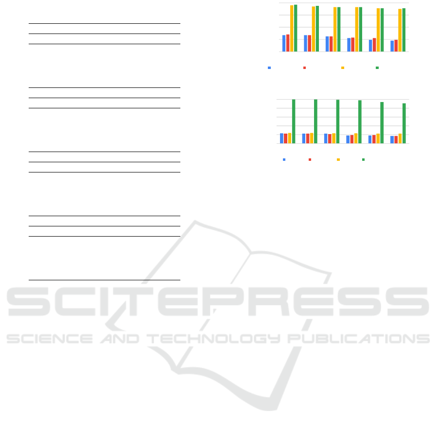
Table 2: Anytime Classification Accuracy (F1-score) for
various datasets with variation in stream speed (λ) at k=15.
FC Dataset
λ (ops) UENO LEMES MVPT AnykNN
10000 0.41 0.42 0.89 0.90
20000 0.33 0.33 0.84 0.84
40000 0.27 0.26 0.79 0.80
60000 0.24 0.24 0.72 0.72
80000 0.18 0.20 0.68 0.67
100000 0.11 0.13 0.65 0.65
PK Dataset
λ (ops) UENO LEMES MVPT AnykNN
10000 0.32 0.33 0.87 0.86
20000 0.24 0.25 0.81 0.80
40000 0.19 0.21 0.76 0.76
60000 0.15 0.20 0.72 0.73
80000 0.13 0.16 0.68 0.69
100000 0.09 0.13 0.63 0.65
SK Dataset
λ (ops) UENO LEMES MVPT AnykNN
10000 0.81 0.81 0.94 0.93
20000 0.75 0.74 0.90 0.90
40000 0.59 0.60 0.83 0.82
60000 0.42 0.43 0.78 0.78
80000 0.31 0.31 0.72 0.73
100000 0.27 0.26 0.68 0.69
KD Dataset
λ (ops) UENO LEMES MVPT AnykNN
10000 0.34 0.35 0.75 0.78
20000 0.32 0.32 0.7 0.75
40000 0.28 0.29 0.69 0.68
60000 0.28 0.28 0.62 0.62
80000 0.25 0.25 0.59 0.58
100000 0.17 0.19 0.44 0.44
on the number of micro-clusters to be indexed. The
results presented in Table 1 clearly show that ANY-k-
NN has very less model training time when compared
to the other methods. UENO and LEMES use sorting
to build their models and are extremely slow. MVPT
uses complex operations to determine the boundary
splits in each node, due to which the construction time
shoots up, in spite of having O(n log n) time complex-
ity. This shows that these three models are not suit-
able for handling large datasets. However, ANY-k-
NN takes very less time with O(n log n) time com-
plexity (with lesser constant term factor). ANY-k-NN
uses multiple trees (one for each class) in its training
model, and the construction of multiple smaller trees
is much faster than building a single tree for the same
dataset, as determined in (Goyal et al., 2020). Hence,
it is more suitable to handle larger datasets.
In the next experiment, we measure the accuracy
of the anytime k-NN classifier for different methods
over three datasets (FC, PK, SK and KD), with vari-
ation in average stream speed (λ) at a fixed value of
k = 15. We use 80% of each dataset to train the cor-
responding training model in a similar non-anytime
offline manner as that of the previous experiment.
The remaining 20% is used as test data, simulated
as a variable speed stream. Table 2 shows that the
classification accuracies (F-1 score) of MVPT and
ANY-k-NN are much better than those of UENO and
LEMES. This is because the class inferencing meth-
0
0.2
0.4
0.6
0.8
k=5 k=10 k=15 k=20 k=25 k=30
F-1 score
UENO LEMES MVPT AnyKNN
Figure 4: F1-score with variation in k at λ= 50k for FC.
0
0.2
0.4
0.6
0.8
1
λ=10k λ=20k λ=40k λ=60k λ=80k λ=100k
F1-score
UENO LEMES MVPT AnyKNN
Figure 5: Measuring F1-score of various methods for vary-
ing (λ), at k = 15, with incremental model update of ANY-
K-NN for SC dataset.
ods of UENO and LEMES require a linear scan of
the training model, which performs very poorly when
the dataset size is large. Whereas MVPT and ANY-k-
NN use hierarchical classification models, which per-
form better than the previous ones. The classification
accuracies of MVPT and ANY-k-NN are very much
close to each other for all datasets at all values of λ.
However, we should note that the model construction
time of MVPT is very high compared to ANY-k-NN.
This means that ANY-k-NN achieves higher accuracy
with lower model construction time. Also, MVPT,
UENO, and LEMES don’t support incremental model
updates, concept drift and class evolution. This shows
that ANY-k-NN is superior to others.
An important thing to be noted from the results
presented in Table 2 is that the F1 values for the
KD dataset are low for all the methods even at lower
stream speeds. This is because of its large dimen-
sionality. At high dimensions, the euclidean distance
measure fails, due to which the results produced are
not very accurate. However, one can note that ANY-k-
NN consistently performs better than the other meth-
ods for the reasons stated above. Also, using the par-
allel framework ANY-MP-k-NN improves the overall
accuracy for this dataset as stated in Table 6.
In the next experiment, we measure the Classifica-
tion accuracy (F1-score) of all the models with varia-
tion in k at a fixed average stream speed (λ = 50,000
ops) for the FC dataset. A similar 80:20 data split has
been used for training and testing as the previous ex-
periment. The results presented in Fig.4 clearly show
that for all values of k, ANY-k-NN and MVPT pro-
duce higher accuracies than UENO and LEMES for
similar reasons explained in the previous experiment.
Note that similar observations were obtained for other
datasets as well.
ICAART 2024 - 16th International Conference on Agents and Artificial Intelligence
284

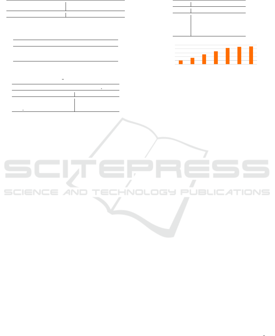
Table 3: Anytime Classification Accuracy (F1-Score) for
ANY-k-NN with and without using geometric time frames
at λ=50k for SC.
F1-Score without Geometric
Time Frame
F1-Score using Geometric Time
Frames
0.87 0.94
Table 4: Memory occupied by various methods for different
datasets.
Dataset(s) UENO LEMES MVPT AnykNN
FC 169 MB 172 MB 754 MB 1069 MB
PK 306 MB 325 MB 1072 MB 1789 MB
SK 72 MB 74 MB 152 MB 189 MB
Table 5: Memory vs F1-score at λ=40k, with & without
bounding the memory (max mc=50k).
AnykNN AnykNN (max mc=50k)
Dataset(s) Memory F1 Memory F1
Forest Cover 1069 MB 0.8 498 MB 0.79
Poker 1789 MB 0.76 847 MB 0.76
Skin Nonskin 189 MB 0.82 117 MB 0.81
In the next experiment, we demonstrate the capa-
bility of ANY-k-NN to handle class evolution in the
streams. We also demonstrate the benefits of incre-
mental model updates. These two features are not
present in the UENO, LEMES, and MVPT. For this
experiment, we create a synthetic classes dataset (SC)
that contains five well-separated Gaussian clusters,
with each cluster treated as a separate class. We start
training our models on 20% of the data containing
objects only from classes 1 and 2. For ANY-k-NN
we use non-anytime offline mode of construction like
previous experiments. The remaining 80% of the ob-
jects (including the objects of other classes) arrive in
the stream. Of these stream objects, 80% are labeled,
and 20% are unlabelled. The labelled objects are used
to incrementally update the model in the case of ANY-
k-NN but are not utilized in the other methods. Also,
when labelled objects arriving in the stream belong to
classes 3, 4, and 5 (whose objects are not present in
the initial training model), ANY-k-NN uses them to
build separate Any-NN-trees for each newly evolving
class. This feature is not present in the other methods.
The unlabelled objects are used for class inference.
The results presented in Fig.5 clearly show that at all
stream speeds, ANY-k-NN produces far better clas-
sification accuracy. This is attributed to incremental
model updates and the capture of evolving classes.
In the next experiment, we demonstrate the cap-
ture of concept drift using geometric time frames us-
ing the SC dataset, which has 5 Gaussian clusters, say
C1, C2, C3, C4 and C5. The initial training model
(constructed with 70% data) uses most points (>70%)
from C1, C2, C3 & C4, but only 20% of points from
C5. The remaining objects arrive in the stream. We
set the stream speed to λ=50,000 ops. We divide the
Table 6: Measuring F1-score for ANY-MP-k-NN with in-
crease in # of parallel streams at different values of λ for
KD dataset.
# Parallel Streams
λ (ops) 4 8 16 32
10k 0.91 0.91 0.91 0.92
20k 0.89 0.91 0.91 0.92
30k 0.85 0.90 0.89 0.92
40k 0.79 0.86 0.87 0.89
50k 0.72 0.85 0.86 0.89
0. 00
0. 20
0. 40
0. 60
0. 80
1. 00
1 4 8 16 32 64 12 8
F-1 score
No of Computing Nodes / Parallel Streams
Figure 6: Measuring F1-score for ANY-MP-k-NN with an
increase in the number of computing nodes while handling
same overall stream speed for SL dataset.
stream into snapshots of approx 0.1 second each, giv-
ing a total of 30 snapshots stored in the geometric
time frames when the stream is received. We mea-
sure the classification accuracy with and without us-
ing the geometric time frame information, wherein we
choose the time horizon containing the last 10 snap-
shots to classify the test instances. The results pre-
sented in Table 3 clearly show that the classification
accuracy while using geometric time frames is bet-
ter as it uses the most recently arrived stream objects
for class inference especially for objects that belong
to the class C5 that arrive mostly in the stream. This
experiment thus demonstrates the capture of concept
drift by the proposed method.
In the next experiment, we measure the peak heap
memory consumed by all the methods as shown in
Table 4. The respective models are constructed over
80% data for all the datasets. The results show that
the ANY-k-NN has the highest memory consump-
tion. MVPT and ANY-k-NN use hierarchical index-
ing structures for indexing data, which leads to larger
memory consumption. Usage of buffers, geomet-
ric time frames at each micro-cluster consumes ad-
ditional memory in the case of ANY-k-NN. Larger
memory consumption for ANY-k-NN when com-
pared to others is very well justified, given that it pro-
duces higher classification accuracy, handles concept
drift and class evolution.
In the next experiment, we study the behaviour of
ANY-k-NN when we use the feature of limiting the
number of micro-clusters indexed in the tree. The
train:test ratio is 80:20. The results presented in Ta-
ble 5 show that even when we limit the number of
micro-clusters formed to 50,000 (value of max mc)
in the entire forest, there is no compromise on the
classification accuracy. Hence, this feature of limiting
the number of micro-clusters is an important feature
A Hierarchical Anytime k-NN Classifier for Large-Scale High-Speed Data Streams
285

that can be applied to limit memory consumption and
thus avoid the exploding memory problem while han-
dling streams. The parameter max mc can be varied
as per the user preferences depending upon the avail-
able memory constraint.
In the next experiment, we measure the Classifi-
cation accuracy (F1-score) of ANY-MP-k-NN at dif-
ferent stream speeds for the KD dataset, with an in-
crease in the number of parallel streams, each handled
in a separate computing node. 20% of the data has
been used to construct the initial training model be-
fore starting the stream at each computing node. We
set the syncing interval γ = 0.50 seconds. max MP mc
is set to 50,000. In each observation, every computing
node receives the stream with the same average speed
(λ) specified in Table 6. The results presented in Ta-
ble 6 show that the classification accuracy improves
with an increase in the number of parallel streams,
especially at higher stream speeds. This is expected
because increasing the number of parallel streams in-
creases the granularity of the overall classifier model
as the degree of data aggregation is reduced. This
makes the classifier more accurate for a higher num-
ber of streams.
In the next experiment, we split a single stream
into multiple streams ranging between 4 and 32 and
measure the anytime classifier accuracy of ANY-MP-
k-NN. We choose the SL dataset and set λ=320,000
ops. This stream is split into multiple streams. For
example, if we split it into 4 streams, each stream
has a speed of 80,000 ops. max MP mc is set to
50,000. The results presented in Fig. 6 clearly show
that the classification accuracy improves greatly as
we split the stream into a higher number of streams.
This is because as the stream is split amongst multiple
computing nodes, it allows for greater refinement and
lesser aggregation of the Any-NN-trees present at each
computing node. The classification accuracy while
using a lesser number of computing nodes was signif-
icantly low and was useless. Such large data streams
can only be handled accurately when multiple com-
puting nodes execute ANY-MP-k-NN as illustrated
in Fig.6. This shows the effectiveness of ANY-MP-
k-NN in handling extremely large and high-speed
streams.
7 CONCLUSION
In this paper, we presented ANY-k-NN, an anytime
k-NN classifier method designed for data streams. It
uses a proposed hierarchical structure, Any-NN-forest,
a collection of c Any-NN-trees for indexing the train-
ing data, as its classification model. The experimen-
tal results show that ANY-k-NN effectively infers the
class labels of the test objects arriving in the stream
with varying inter-arrival rates. The experimental re-
sults also suggest that ANY-k-NN can handle very
large data streams, capable of incrementally updat-
ing its classification model, and effectively handles
concept drift and class evolution, all of this while not
letting the memory consumption explode. We have
also presented a parallel framework ANY-MP-k-NN,
which is the first of its kind framework for anytime
k-NN classification of multi-port data streams over
distributed memory architectures. The experimental
results show its effectiveness in handling multi-port,
large-size, and very high-speed data streams.
In the future, we plan to implement bulk-loading
R-tree methods for model construction to improve
classification accuracy further. We also extend this
method to other parallel architectures such as shared
memory and GP-GPUs.
REFERENCES
Aggarwal, C. C., Han, J., Wang, J., and Yu, P. S.
(2004). On demand classification of data streams. In
Proceedings-ACM SIGKDD, pages 503–508.
Alberghini, G., Barbon Junior, S., and Cano, A. (2022).
Adaptive ensemble of self-adjusting nearest neighbor
subspaces for multi-label drifting data streams. Neu-
rocomputing, 481:228–248.
Bentley, J. L. (1975). Multidimensional Binary Search
Trees Used for Associative Searching. Communica-
tions of the ACM, 18(9):509–517.
Blackard, J. A. and Dean, D. J. (1999). Comparative ac-
curacies of artificial neural networks and discriminant
analysis in predicting forest cover types from carto-
graphic variables. Computers and Electronics in Agri-
culture, 24(3):131–151.
Bozkaya, T. and Ozsoyoglu, M. (1999). Indexing Large
Metric Spaces for Similarity Search Queries. ACM
Trans. on Database Systems, 24(3):361–404.
Cattral, R., Oppacher, F., and Deugo, D. (2002). Evolu-
tionary data mining with automatic rule generaliza-
tion. Recent Advances in Computers, Computing and
Communications, 1(1):296–300.
Challa, J. S., Goyal, P., Giri, V. M., Mantri, D., and Goyal,
N. (2019). AnySC: Anytime Set-wise Classification of
Variable Speed Data Streams. In Proceedings - IEEE
Big Data, pages 967–974.
Challa, J. S., Goyal, P., Kokandakar, A., Mantri, D., Verma,
P., Balasubramaniam, S., and Goyal, N. (2022a). Any-
time clustering of data streams while handling noise
and concept drift. Journal of Experimental and Theo-
retical Artificial Intelligence, 34(3):399–429.
Challa, J. S., Rawat, D., Goyal, N., and Goyal, P. (2022b).
Anystreamkm: Anytime k-medoids clustering for
streaming data. In Proceedings - IEEE Big Data,
pages 844–853.
ICAART 2024 - 16th International Conference on Agents and Artificial Intelligence
286

Cover, T. M. and Hart, P. E. (1967). Nearest Neighbor Pat-
tern Classification. IEEE Trans. on Information The-
ory, 13(1):21–27.
de Barros, R. S. M., Santos, S. G. T. d. C., and Barddal, J. P.
(2022). Evaluating k-NN in the Classification of Data
Streams with Concept Drift. arxiv.org, 1.
DeCoste, D. (2012). Anytime Interval-Valued Outputs for
Kernel Machines: Fast Support Vector Machine Clas-
sification via Distance Geometry. In Proceedings of
the 19th ICML, volume 9, pages 99–106.
Duda, R. O., Hart, P. E., and Stork, D. G. (2000). Pattern
Classification. Wiley.
Esmeir, S. and Markovitch, S. (2007). Anytime induction of
cost-sensitive trees. Advances in Neural Information
Processing Systems, 20.
F1-score. F1-score https://en.wikipedia.org/wiki/F-score.
Ferchichi, H. and Akaichi, J. (2016). Using Mapreduce for
Efficient Parallel Processing of Continuous K nearest
Neighbors in Road Networks. Journal of Software and
Systems Development, pages 1–16.
Goyal, P., Challa, J. S., Kumar, D., Bhat, A., Balasubra-
maniam, S., and Goyal, N. (2020). Grid-R-tree: a
data structure for efficient neighborhood and nearest
neighbor queries in data mining. JDSA, 10(1):25–47.
Guttman, A. (1984). R-trees: A dynamic index structure for
spatial searching. ACM SIGMOD Record, 14(2):47–
57.
Hidalgo, J. I. G., Santos, S. G. T., and de Barros, R. S. M.
(2023). Paired k-NN learners with dynamically ad-
justed number of neighbors for classification of drift-
ing data streams. KAIS, 65(4):1787–1816.
Hjaltason, G. R. and Samet, H. (1999). Distance browsing
in spatial databases. ACM Transactions on Database
Systems, 24(2):265–318.
Hu, H., Dey, D., Hebert, M., and Andrew Bagnell, J. (2019).
Learning anytime predictions in neural networks via
adaptive loss balancing. In 33rd AAAI Conference,
pages 3812–3821.
KDD CUP (1999). http://kdd.ics.uci.edu/databases/ kdd-
cup99/kddcup99.html.
Kranen, P., Assent, I., Baldauf, C., and Seidl, T. (2011a).
The ClusTree: Indexing micro-clusters for anytime
stream mining. Knowledge and Information Systems,
29(2):249–272.
Kranen, P., Hassani, M., and Seidl, T. (2012). BT* -
An advanced algorithm for anytime classification. In
Proceedings-SSDM, pages 298–315.
Kranen, P., Reidl, F., Villaamil, F. S., and Seidl, T. (2011b).
Hierarchical clustering for real-time stream data with
noise. In Proceedings - SSDBM, page 405–413.
Lemes, C. I., Silva, D. F., and Batista, G. E. (2014). Adding
diversity to rank examples in anytime nearest neighbor
classification. In Proceedings - 13th ICMLA, pages
129–134.
MPI. MPI : A message-passing interface standard
https://www.mcs.anl.gov/research/projects/mpi/.
Nair, P. and Kashyap, I. (2020). Classification of medical
image data using k nearest neighbor and finding the
optimal k value. Int. Journal of Scientific and Tech-
nology Research, 9(4):221–226.
Ram
´
ırez-Gallego, S., Krawczyk, B., Garc
´
ıa, S., W
´
ozniak,
M., Ben
´
ıtez, J. M., and Herrera, F. (2017). Nearest
neighbor classification for high-speed big data streams
using spark. IEEE Trans on Systems, Man, and Cyber-
netics: Systems, 47(10):2727–2739.
Roseberry, M., Krawczyk, B., Djenouri, Y., and Cano, A.
(2021). Self-adjusting k nearest neighbors for con-
tinual learning from multi-label drifting data streams.
Neurocomputing, 442:10–25.
Rossi, R. A. and Ahmed, N. K. (2015). The network data
repository with interactive graph analytics and visual-
ization. In Proceedings - AAAI, page 4292–4293.
Shinde, A. V. and Patil, D. D. (2023). A Multi-Classifier-
Based Recommender System for Early Autism Spec-
trum Disorder Detection using Machine Learning.
Healthcare Analytics, 4(June):100211.
Sun, Y., Pfahringer, B., Gomes, H. M., and Bifet, A. (2022).
Soknl: A novel way of integrating k-nearest neigh-
bours with adaptive random forest regression for data
streams. Data Mining and Knowledge Discovery,
36(5):2006–2032.
Susheela Devi, V. and Meena, L. (2017). Parallel MCNN
(pMCNN) with Application to Prototype Selection on
Large and Streaming Data. JAISCR, 7(3):155–169.
Ueno, K., Xi, A., Keogh, E., and Lee, D. J. (2006). Any-
time classification using the nearest neighbor algo-
rithm with applications to stream mining. In Proceed-
ings - IEEE ICDM, pages 623–632.
Venkataravana Nayak, K., Arunalatha, J., and Venugopal,
K. (2021). Ir-ff-knn: Image retrieval using feature
fusion with k-nearest neighbour classifier. In 2021
Workshop on Algorithm and Big Data, page 86–89.
Wu, G., Zhao, Z., Fu, G., Wang, H., Wang, Y., Wang, Z.,
Hou, J., and Huang, L. (2019). A fast k nn-based ap-
proach for time sensitive anomaly detection over data
streams. In Proceedings-ICCS, pages 59–74.
Xu, W., Miranker, D. P., Mao, R., and Ramakrishnan,
S. (2008). Anytime K-nearest neighbor search for
database applications. In Proceedings - International
Workshop on SISAP, pages 139–148.
A Hierarchical Anytime k-NN Classifier for Large-Scale High-Speed Data Streams
287