Real-Time Bus Arrival Prediction: A Deep Learning Approach for

Enhanced Urban Mobility

Narges Rashvand

, Sanaz Sadat Hosseini

, Mona Azarbayjani

and Hamed Tabkhi

Department of Electrical and Computer Engineering, University of North Carolina at Charlotte, Charlotte, NC, U.S.A.

Department of Civil and Environmental Engineering, University of North Carolina at Charlotte, Charlotte, NC, U.S.A.

Department of Architecture, University of North Carolina at Charlotte, Charlotte, NC, U.S.A.

Keywords:

Neural Network, Feature Selection, Bus Arrival Time, Support Vector Regression.

Abstract:

In urban settings, bus transit stands as a signiﬁcant mode of public transportation, yet faces hurdles in deliver-

ing accurate and reliable arrival times. This discrepancy often culminates in delays and a decline in ridership,

particularly in areas with a heavy reliance on bus transit. A prevalent challenge is the mismatch between ac-

tual bus arrival times and their scheduled counterparts, leading to disruptions in ﬁxed schedules. Our study,

utilizing New York City bus data, reveals an average delay of approximately eight minutes between scheduled

and actual bus arrival times. This research introduces an innovative, AI-based, data-driven methodology for

predicting bus arrival times at various transit points (stations), offering a collective prediction for all bus lines

within large metropolitan areas. Through the deployment of a fully connected neural network, our method

elevates the accuracy and efﬁciency of public bus transit systems. Our comprehensive evaluation encompasses

over 200 bus lines and 2 million data points, showcasing an error margin of under 40 seconds for arrival time

estimates. Additionally, the inference time for each data point in the validation set is recorded at below 0.006

ms, demonstrating the potential of our Neural-Net based approach in substantially enhancing the punctuality

and reliability of bus transit systems.

1 INTRODUCTION

Over the last half-century in the US, the share of

workers commuting via public transportation has

dwindled. This decline is largely ascribed to govern-

mental separation of land-use development planning

from transportation, fueling suburban sprawl, uneven

public service distribution, and escalating car reliance

in many American cities (Freemark, 2021; Pulugurtha

et al., 2022). Despite concerted efforts over re-

cent decades to bolster public transportation, rider-

ship in the United States hasn’t witnessed a signiﬁcant

uptick, falling below anticipated levels. This stagna-

tion is driven by factors such as urban sprawl, sub-

urbanization, private car ownership, low fuel prices,

cutbacks in transit services, and the emergence of

ride-hailing giants like Uber and Lyft (Erhardt et al.,

2022; Graehler et al., 2019).

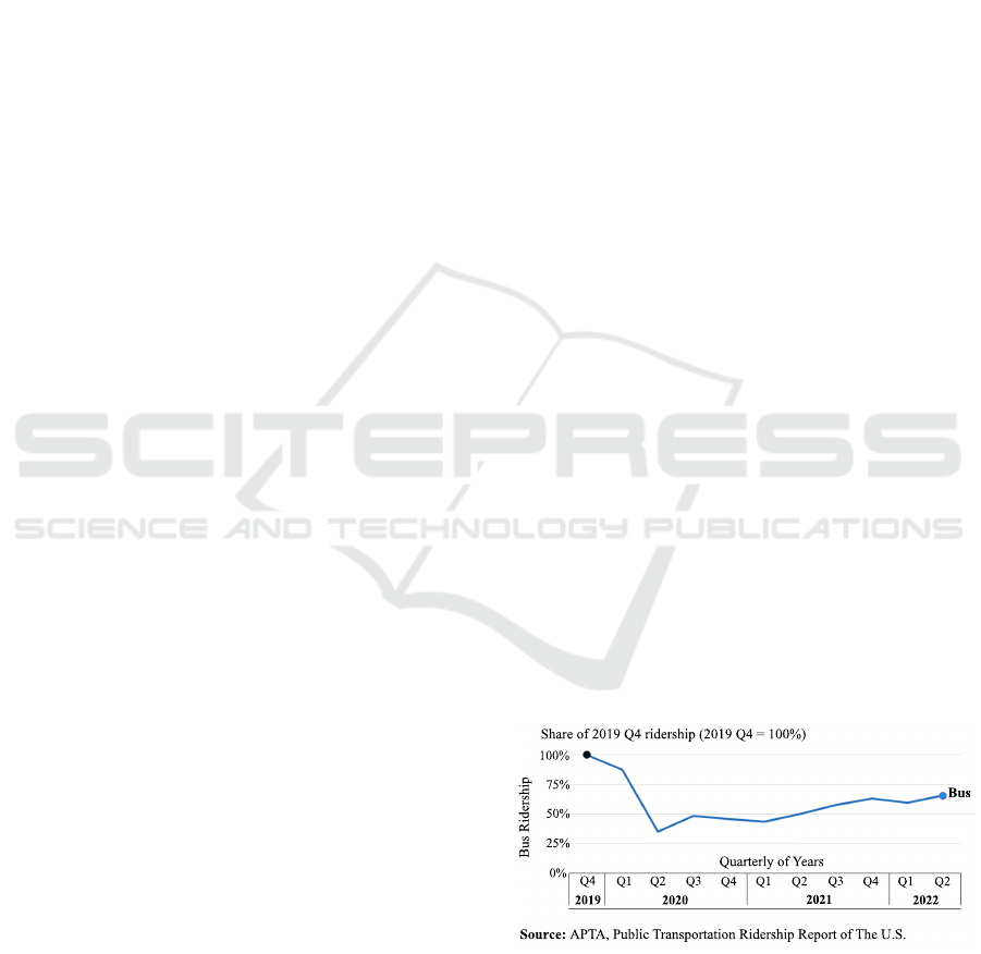
The recent COVID-19 pandemic has further exac-

erbated the decline in bus ridership across the coun-

try, deteriorating the situation from its prior state. The

American Public Transportation Association (APTA)

notes a stark reduction in transit usage due to the pan-

demic, with a downturn of over 50 percent between

2019 and 2020 (Figure 1). However, there’s a silver

lining post-pandemic; public transportation ridership

in the U.S. has rebounded from 19% in April 2020

to 72% in September 2022, marking the highest level

since 2019 (Mallett, 2022; APT, 2022).

Bus Ridership

Quarterly of Years

Share of 2019 Q4 ridership (2019 Q4 = 100%)

Bus

Q1 Q2 Q3

Q4 Q1 Q2

2019 2020

2021

100%

75%

50%

25%

2022

Source: APTA, Public Transportation Ridership Report of The U.S.

Figure 1: Quarterly Public Bus Transportation Ridership in

the U.S. In 2020 and 2021, public transportation ridership

was less than half its pre-pandemic level. While bus rid-

ership has recovered somewhat, it was much lower in the

second quarter of 2022 than in the ﬁnal pre-pandemic quar-

ter. Bus ridership for commuters grew by 66% in the second

quarter of 2022 (Mallett, 2022).

Rashvand, N., Hosseini, S., Azarbayjani, M. and Tabkhi, H.

Real-Time Bus Arrival Prediction: A Deep Learning Approach for Enhanced Urban Mobility.

DOI: 10.5220/0012365500003639

Paper published under CC license (CC BY-NC-ND 4.0)

In Proceedings of the 13th International Conference on Operations Research and Enterprise Systems (ICORES 2024), pages 123-132

ISBN: 978-989-758-681-1; ISSN: 2184-4372

123

The burgeoning discourse around smart cities has

piqued the interest of scholars across diverse ﬁelds

(Pazho et al., 2023; Gholami et al., 2023; Noghre

et al., 2022). Central to the smart city paradigm

is transit reliability, a critical consideration for com-

muters aiming to minimize long commutes and wait-

ing times on public transit.

To cater to individuals heavily reliant on public

transit, developed cities globally are honing their tran-

sit scheduling systems. As previously discussed, nu-

merous factors can inﬂuence transit ridership, with

service predictability being paramount to mitigate un-

due wait times and enhance trip planning reliability

(Pulugurtha et al., 2022; Sen et al., 2022). Unre-

liable transit services can thwart commuters’ travel

plans, potentially prompting a shift to alternative

transportation modes like personal vehicles. Op-

erational uncertainties and delays may erode tran-

sit users’ conﬁdence, resulting in reduced ridership

and increased dependence on alternative transporta-

tion modes. Such unreliable services compel transit

users to allocate more time for waiting, culminating in

extended wait durations at transit stops (Xu and Ying,

2017; Huang et al., 2022; Zhong et al., 2020).

Many cities have rolled out dedicated mobile ap-

plications for bus transit, furnishing schedules and

aiding passengers in pre-planning their journeys (Fu

et al., 2014). However, the absence of real-time infor-

mation in these apps often vexes passengers attempt-

ing to plan their commute. A sizeable number of

commuters resort to other applications (e.g., Google

Maps or Waze (spl, 2023)) for planning their tran-

sit. Nonetheless, these applications, reliant on crowd-

sourced information, often fall short in providing req-

uisite accuracy and don’t liaise with local bus transits

to bolster scheduling and operational efﬁciency (spl,

2023).

Public transit holds the promise of delivering real-

time estimated arrival times akin to private sector

ride-sharing platforms like Uber or Lyft (Chen et al.,

2015; TSG, 2019). Smart, data-driven stratagems

could potentially elevate predictability and efﬁciency

across public bus transit systems, mirroring the reli-

ability and predictability seen in Uber/Lyft. The req-

uisite steps encompass regional data gathering, anal-

ysis, pattern discernment, and forecasting to augment

arrival time accuracy and bus trip planning across the

entire network. By doing so, transit authorities could

potentially boost ridership, fostering a more sustain-

able and cost-effective alternative to personal vehicle

use, thereby contributing to a greener and more equi-

table society (Diab et al., 2015; tel, 2017).

This manuscript unveils a deep-learning-centric

model for predicting bus arrival times, employing

a uniﬁed Fully Connected Neural Networks (FC-

NNs) framework based on historical and environmen-

tal data. This model exhibits robust scalability and

generalization across numerous bus lines within iden-

tical transit networks, surpassing the capabilities of

classical machine learning methodologies. Utilizing

the New York City Bus System Dataset, encompass-

ing over 200 bus lines and 2 million data points, we

conducted our analysis.

Our ﬁndings elucidate that our AI-powered model,

anchored in FCNNs, signiﬁcantly curtails the aver-

age estimated error in bus arrival times to 40 seconds,

a noteworthy improvement compared to the average

delay times in the dataset. Per our study, FCNNs

outshine traditional machine learning approaches like

SVR in tackling transportation conundrums with ex-

tensive input features.

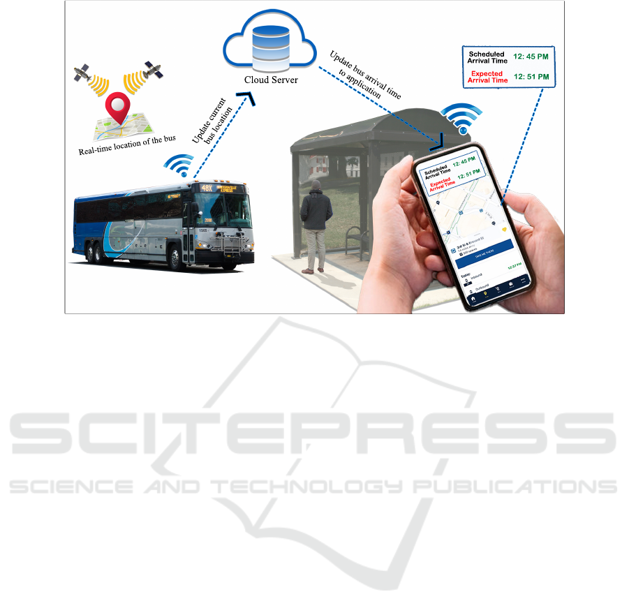
The quintessence of this endeavor is to seamlessly

assimilate the developed model into existing public

bus transit mobile applications, as depicted in Figure

2, with the overarching aim of enriching the bus tran-

sit experience. By leveraging this methodology, we

aspire to substantially diminish waiting times for pas-

sengers, thereby enhancing their commuting experi-

ence.

In summary, the contributions of this paper en-

compass:

• The introduction of a uniﬁed, deep-learning-based

Fully Connected Neural Network (FCNN) frame-

work aimed at predicting bus arrival times across

numerous bus lines within a singular bus transit

network.

• The thorough assessment of the proposed model’s

accuracy utilizing the expansive New York City

Bus System Dataset, which comprises more than

200 bus lines and 2 million data points.

• The illustration of our methodology’s superior

scalability and generalization capabilities when

juxtaposed with classical machine learning mod-

els such as Support Vector Machines.

The rest of this paper is structured as follows: The

subsequent section is devoted to bus arrival time

prediction literature review. The preliminaries and

dataset section contains a detailed description of the

dataset used in this study and some exploratory data

analysis. Our methodology is illustrated in the pro-

posed neural network methodology section. Finally,

our model is validated, and we present our conclu-

sions in the last section.

ICORES 2024 - 13th International Conference on Operations Research and Enterprise Systems

124

Scheduled

Arrival Time

Expected

Arrival Time

12: 45 PM

12: 51 PM

Scheduled

Arrival Time

Real-time location of the bus

Cloud Server

Update current

bus location

Update bus arrival time

to application

Expected

Arrival Time

12: 45 PM

12: 51 PM

Figure 2: Integrating an AI prediction model into a mobile bus app enhances user experience and operational efﬁciency.

Our model predicts bus arrival times using diverse data sources, providing real-time precision. Users can easily access these

predictions via cloud-based services for a reliable travel experience.

2 RELATED WORKS

Our objective in this section is to assess the efﬁciency

of examples similar to our research demonstrating

how data-driven approaches can be used for bus tran-

sit systems, arrival time prediction, and scheduling

optimization. Public transportation is a crucial com-

ponent of a connected and smart community. There-

fore, citizens demand real-time information regard-

ing transportation assets’ arrival and departure. In

many cities worldwide, intelligent transportation sys-

tems with demand-responsive services are being im-

plemented to bridge the gap between public trans-

portation and private cars. In some early research,

data analytics has been used to optimize public bus

schedules and minimize passenger wait times.

Different technologies can be utilized that could

generate real-time data for bus arrival time prediction.

Among them, Global Positioning Systems (GPS), Au-

tomatic Passengers Counter Systems (APCS), and

Crowdsensing solutions in which users cooperate

with the system through a mobile application are the

most popular ones (Gaikwad and Varma, 2019; Yin

et al., 2017).

The problem of bus arrival time prediction was

studied by considering different models and various

essential factors. In a study by N. Gaikwad and S.

Varma (Gaikwad and Varma, 2019), the crucial fea-

tures for bus arrival time prediction and standard eval-

uation metrics were presented. The main factors af-

fecting bus arrival time are the source, destination,

bus location coordinates, trafﬁc density, stop-to-stop

distance, workday, and so on.

In another study by Raﬁdah Md.(Noor et al.,

2020), bus arrival time was predicted using the Sup-

port Vector Regression (SVR) model. Petaling Jaya

City Bus data was used in this study, including a se-

quence of bus stations, bus station names, the coordi-

nates of the bus stations, timestamps, and the distance

covered from the previous station to the next station.

They also implemented their prediction model with

and without weather data and showed that adding

weather parameters for their dataset shows a negligi-

ble difference in their prediction error.

Also, a study by F. Sun, Y. Pan, J. White, and A.

Dubey (Sun et al., 2016) introduced a public trans-

portation decision support system for short-term and

long-term prediction of arrival bus times. This study

used the real-world historical data of two Nashville

bus system routes. The approach of this research

combined the clustering analysis and Kalman ﬁlters

with a shared route segment model to produce more

accurate arrival time predictions and, based on their

results, compared to the basic arrival time prediction

model that Nashville MTA was using, their system

reduced arrival time prediction errors by 25% on av-

erage when predicting the arrival delay an hour ahead

and 47% when predicting within a 15-minute future

Real-Time Bus Arrival Prediction: A Deep Learning Approach for Enhanced Urban Mobility

125

time window (Sun et al., 2016).

S. Basak, F. Sun, S. Sengupta, and A. Dubey

have conducted a similar study (Dubey et al., 2019),

using unsupervised clustering mechanisms to opti-

mize transit on-time performance. As a local case

study, they analyzed the monthly and seasonal delays

of the Nashville metro region and clustered months

with similar patterns. In this paper, they presented

a stochastic optimization toolchain along with sensi-

tivity analyses for choosing the optimal hyperparam-

eters, and they solved the optimization problem by

using a single-objective optimization task as well as

a greedy algorithm, a genetic algorithm (GA), and a

particle swarm optimization (PSO) algorithm (Dubey

et al., 2019).

According to the newest research in (Sun et al.,

2019), dynamic data-driven application systems

(DDDAS) that use real-time sensors and a data-driven

decision support system can provide online model

learning and multi-time-scale analytics to enhance the

system’s intelligence. As part of their study, the au-

thors analyzed an online bus arrival prediction system

in Nashville using historical and real-time streaming

data, which can be packaged as modular, distributed,

and resilient micro-services. The long-term delay

analysis service excludes noise from outliers in his-

torical data to identify delay patterns associated with

different hours, days, and seasons for speciﬁc time

points and route segments. City planners can use the

feedback data generated by these analytics services to

improve bus schedules and increase rider satisfaction

(Sun et al., 2019).

In addition, another study by S. Nannapaneni and

A. Dubey (Nannapaneni and Dubey, 2019) researched

rerouting a single bus to serve spatially and tempo-

rally better changing travel demands. The aim was to

propose a ﬂexible framework for public transit rerout-

ing. The study was demonstrated on Route 7 of the

Nashville Metropolitan Transit Authority (MTA). The

authors identiﬁed several ﬂex stops with high travel

demand using clustering since people living far from

bus routes tend to choose alternate transit modes,

leading to increased trafﬁc congestion. They catego-

rized the bus stops along the static routes into critical

and non-critical stops and added slack time to account

for travel delays during the existing static scheduling

process. As a result, ﬂexible routes resulted in less

additional travel time than available slack time. The

effectiveness of rerouting was analyzed using the per-

centage increase in travel demand (Nannapaneni and

Dubey, 2019).

3 PRELIMINARIES AND

DATASET

3.1 Dataset Description

The dataset is a critical component of every AI-based

system. This study utilizes New York City Bus data

(NYC, 2017). A total of 232 bus lines were inspected

to collect this data, and these records were captured

in 10-minute increments from 4468 buses.

This dataset was selected due to its rich proper-

ties. More than 6 million data generated in a month

are included in this dataset. Not only does this data

set have a vast number of records, but it also consists

of the most relevant parameters to the problem of ar-

rival time prediction. Each record contains the infor-

mation in the format of 17 ﬁelds, including Vehicle

location. Longitude, VehicleLocation.Latitude, Des-

tinationLong, DestinationLat, OriginLong, Origin-

Lat, RecordedAtTime, ArrivalTime, ScheduledAr-

rivalTime, DistanceFromStop, OriginName, Des-

tinationName, PublishedLineName, NextStopPoint-

Name, ArrivalProximityText, VehicleRef and Direc-

tionRef. The ﬁrst 6 ﬁelds are the current bus location,

destination, and origin coordinates. Other ﬁeld de-

scriptions are as follows:

• RecordedAtTime is the checkpoint time in which

the current location of the bus is recorded and

used as the bus observation time in this study.

• ArrivalTime is the time when the bus arrives at the

next stop.

• ScheduledArrivalTime is from the published bus

timetable, indicating the scheduled time for the

bus to arrive at the next stop.

• DistanceFromStop is the distance of the bus from

the next stop at the observation time.

• Origin and destination are deﬁned by OriginName

and DestinationName.

• PublishedLineName represents in which line bus

operates.

• NextStopPointName is the name of the next bus

stop.

• ArrivalProximityText shows the current status of

the bus in terms of a text, including at stop, ap-

proaching, and how many miles the bus is away.

• VehicleRef is the reference number for every bus

whose location is being tracked.

• DirectionRef ﬁeld indicates inbound or outbound

bus direction.

ICORES 2024 - 13th International Conference on Operations Research and Enterprise Systems

126

3.2 Cleaning the Data and

Preprocessing

Data is ﬁrst cleaned and preprocessed to get meaning-

ful concepts from this dataset. Then, the most related

features are created, which will be explained in the

methodology section. While around 6 million data

instances are available in this dataset, they can not

be considered logical observations. Since the goal is

to predict the arrival time of the bus to the next sta-

tion, we are only interested in the data points in which

the bus is moving between bus stations. So, data

is ﬁrst ﬁltered based on the ”ArrivalProximityText”

ﬁeld, and data samples with at-stop value dropped

from the data points, where actual arrival time almost

equals the bus observation time. By doing the previ-

ous steps, around 2 million records were available to

work with.

3.3 Analysis of the Data

Different indicators can measure the quality of service

in public transit infrastructures. On-time performance

at stops is an essential factor. Difference time between

scheduled and actual bus arrivals has been selected

as the top reason people avoid bus transit systems in

many cities (Dubey et al., 2019).

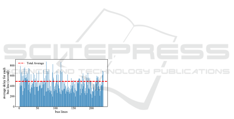
Figure 3: Average delay among all bus lines. Initial analysis

of records in the New York dataset shows that the average

delay across all bus lines equals 491 seconds.

So, data is ﬁrst analyzed regarding mismatching

between the scheduled arrival time and the actual ar-

rival time. Mismatch time refers to any difference

between the bus’s scheduled time and arrival time.

When the bus arrives at the bus stop earlier, passen-

gers might miss the bus, and also, for late buses, pub-

lic transportation infrastructure suffers from the delay.

Any of these two arrival time variations impact com-

muters’ satisfaction signiﬁcantly (Dubey et al., 2019).

Our study found that the average delay and mismatch

time across all lines of this dataset is around 8 minutes

(491 seconds) and 6 minutes, respectively. The aver-

age delay for these 232 bus lines has been illustrated

in Figure 3.

4 PROPOSED NEURAL

NETWORK METHODOLOGY

4.1 Feature Extraction

The New York data set has 232 lines, and each line has

been segmented into the number of bus stops. Assign-

ing each line an integer value would not be a practical

approach since an ordered relationship exists between

integer values and may lead to poor performance of

the model. One-hot encoding applies to categorical

variables like bus lines without an ordinal relation-

ship. This encoding helps the bus lines be injected

into the model in terms of binary variables. Applying

one-hot encoding on bus lines expands the input fea-

tures and adds 232 more inputs. On the other hand,

bus stops have some order, and they are fed into the

model through integer encoding. The bus stop input

variable can help the model track the trafﬁc condi-

tions and passenger ﬂow varying from one bus stop to

another.

As mentioned before, the bus records in this

dataset were collected for a month. Because of the

wide time variation, time is injected into the model in

terms of two categories rather than feeding it directly

into the model. This approach avoids injecting a lot

of noise into the model.

First, based on the day of the bus operation, the

variable ”day type” is added to the input features,

which can get two values, ”weekend” and ”workday”.

The other time-related variable is the rush hour status.

According to the operation time of the bus, this fea-

ture assigns to each record of the dataset, determin-

ing whether the bus operates during rush hour or not.

Rush hour in New York spans from 6 AM to 10 AM

and 3 PM to 7 PM (MTA, 2023).

In addition to the features that were previously

mentioned, there are two distance-related features in

the model. The distance input feature, the most im-

portant feature among other features, indicates how

many meters the bus is far from the next stop. Far

status is another distance-related feature added to in-

put features according to the distance value. It is

a binary feature that changes depending on whether

the distance is below or above a speciﬁed threshold.

Research on the distribution of bus stop spacings in

the United States reveals that the average distance be-

tween bus stops in New York is 328 meters (Pandey

et al., 2021). In our study, we determined a threshold

value of 250 meters through trial and error. when the

distance is below this threshold, it indicates that the

Real-Time Bus Arrival Prediction: A Deep Learning Approach for Enhanced Urban Mobility

127

bus is on its way to the next station and probably not

waiting at the previous bus stop.

Trip time (Tr) is the target variable we aim to pre-

dict with our model, representing the time required

for a bus to reach the next bus station from its current

location. It is calculated in seconds by subtracting

the bus observation time (T

), which corresponds to

the RecordedAtTime in the dataset, from the actual

arrival time (T

), associated with ArrivalTime in the

dataset. In practical scenarios, knowing the trip time

allows for the calculation of the arrival time of the

bus.

Tr = T

− T

(1)

Table 1 summarizes the input and output features that

were produced during the feature extraction step.

Table 1: Input and Output Features.

Input Features

One-hot Encoded Bus Lines

Distance

Day Type

Rush Hour Status

Bus Stops

Far Status

Output Feature Trip Time

4.2 Feature Scaling

Due to the different range of input features, data needs

to be scaled prior to being injected into the model.

Some input features, like rush hour status, are in the

binary form and represented by 1 and 0, while oth-

ers like distance, can be hundreds of meters. Without

feature scaling, the model can be affected by the dif-

ferent range of features, assigning higher weights to

the features with large scale. So, Min-Max scaling is

used to transform the value of all input features to the

range of 0 and 1.

4.3 Train and Validation Sets

The dataset is divided into a train and validation set.

80% of the dataset has been categorized as a training

set for the training of our model, while 20% of the

dataset has been used as a validation set. The total

number of instances is 2.13 million. 1.7 million is

used for training our model, while the rest is utilized

for validation. It is also worth mentioning that the

average of training data samples for each line is 7327.

4.4 Model Design

Artiﬁcial Neural Networks (ANNs) are very common

in forecasting bus trip time. Previous studies have

demonstrated that ANNs are effective in predicting

nonlinear relationships in complicated problems. (Bai

et al., 2015).

In this study, we make use of FCNNs to predict

the bus trip time. As discussed in the previous sec-

tion, due to the large number of bus lines, FCNNs

can handle high-dimensional feature spaces by using

hidden layers and non-linear activation functions. To

determine the optimal architecture for our model, we

conducted various experiments with different conﬁg-

urations, including the number of hidden layers, neu-

rons in each layer, and activation functions. Based on

the results obtained, we selected the best-performing

model with enhanced prediction capabilities.

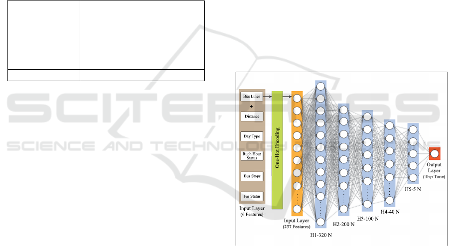
As illustrated in Figure 4, the model is fed with

237 input features, including 232 features generated

through one-hot encoding for bus lines, distance, day

type, rush hour status, bus stops, and far status. Ad-

ditionally, the output layer consists of one neuron

for predicting the bus trip time based on transformed

input data from the preceding hidden layers. Con-

sequently, throughout all our experiments, the input

layer and output layer remained identical.

H1-320 N

H2-200 N

H3-100 N

Output

Layer

(Trip Time)

H4-40 N

H5-5 N

Bus Lines

Distance

Day Type

Bus Stops

Far Status

Ruch Hour

Status

Input Layer

(237 Features)

One-Hot Encoding

Input Layer

(6 Features)

Figure 4: Structure of our model based on the Fully Con-

nected Neural Network. One-hot encoding applies to bus

lines and extends it to 232 features. These converted fea-

tures with other 5 features, including distance, day type,

rush hour status, bus stops, and far status feed to the Fully

Connected Neural Network. The proposed model consists

of 5 hidden layers and ReLU as an activation function. The

number of neurons in each hidden layer can also be seen

in the ﬁgure. H1-320N indicates that the ﬁrst hidden layer

consists of 320 neurons.

Our experimental methodology involved a thor-

ough investigation into the architecture of the neu-

ral network. Speciﬁcally, we systematically varied

the number of hidden layers from 2 to 7, evaluat-

ing their impact on model performance. Within each

ICORES 2024 - 13th International Conference on Operations Research and Enterprise Systems

128

conﬁguration, we adjusted the number of neurons in

a descending order across layers, with the ﬁrst layer

having the maximum number of neurons and the last

layer having the minimum number of neurons. By

modifying these architectural parameters, our goal

was to create a balance between model complexity

and generalization. This aimed to ensure that the

FCNN captures intricate patterns in the data without

overﬁtting.

Our experiments demonstrated that surpassing 5

hidden layers fails to enhance accuracy. Conse-

quently, we utilized 5 hidden layers for our model.

Concerning the number of neurons for each layer, we

observed that an increased number of neurons, 512

neurons, did not yield an improvement in accuracy.

Instead, it led to a more complex model with more

parameters without any beneﬁt in predictive perfor-

mance. Consequently, we settled on 320 neurons for

the ﬁrst layer, ensuring an optimal balance between

capturing complexity and preventing unnecessary pa-

rameter inﬂation. The same rationale guided our de-

cisions in determining the most suitable number of

neurons for each layer.

Moreover, another important factor in FCNNs is

the choice of activation function that plays a key role

by introducing non-linearity to the model. Rectiﬁed

Linear Unit (ReLU) function is used as an activation

function in our model. Since the number of hidden

layers in our model is large, ReLU is a better choice

than Sigmoid and Hyperbolic Tangent (Tanh), helping

to mitigate the vanishing gradient problem.

According to Figure 4, our best model has seven

layers, including an input layer, 5 hidden layers, and

an output layer. In the ﬁrst hidden layer, the model

learns more complex representations of input features

by increasing neurons to 320. The number of neurons

decreases step by step in the next hidden layers, from

200 in the second hidden layer to 5 neurons in the ﬁfth

hidden layer. The structure of the presented model

can be seen in Table 2.

Table 2: Structure of fully connected neural network ap-

plied to New York dataset with 232 bus lines.

Parameters

Number of inputs 237

Number of hidden layers 5

Activation function ReLU

Number of neurons in the ﬁrst layer 320

Number of neurons in the second layer 200

Number of neurons in the third layer 100

Number of neurons in the fourth layer 40

Number of neurons in the ﬁfth layer 5

Number of outputs 1

5 RESULTS AND DISCUSSION

5.1 Performance Measurements

The performance evaluation of arrival time predicted

by the model can be done using different measures,

including Mean Absolute Percentage Error (MAPE),

Mean Square Error (MSE), and Root Mean Square

Error (RMSE).

In this study, we assess the model’s accuracy using

RMSE, which quantiﬁes the difference between pre-

dicted trip times and actual trip times in seconds.

RMSE is a widely used metric in the ﬁeld of bus

arrival time analysis, facilitating comparisons with

other models. Furthermore, RMSE shares the same

unit as the predicted values (seconds), simplifying the

interpretation of errors in terms of time.

RMSE can be represented as the following equa-

tion where t

act

is the actual bus trip time, (Tr in Equa-

tion 1), t

pred

stands for the predicted bus trip time

based on the proposed model, and n is the sample size

for prediction. Lower RMSE represents better perfor-

mance in prediction.

RMSE =

i=1

act

−t

pred

)

(2)

5.2 Results and Model Performance

Discussion

5.2.1 Results for Fully Connected NN on all Bus

Lines

The training process was implemented on a system

with an Intel i7-1185G7 processor with 4 cores and

a speed of 3.00 GHz. Table 3 shows the results of

applying our model on 232 bus lines with the learning

rate of 1e − 2.

Table 3: Obtained results in terms of RMSE for the New

York dataset with 232 bus lines.

Results

Training RMSE 35.69 s

Validation RMSE 35.74 s

It can be observed that the average RMSE for all

bus lines is 35.74 seconds. In other words, the pre-

dicted arrival time of the bus to the next station has

an error lower than 36 seconds. This prediction er-

ror can be contrasted with the average delay observed

across all bus lines in the dataset, which equals to 491

seconds according to the data analysis section. Figure

5 demonstrates the RMSE over each bus line. While

the highest prediction error is 119.99 seconds in line

Real-Time Bus Arrival Prediction: A Deep Learning Approach for Enhanced Urban Mobility

129

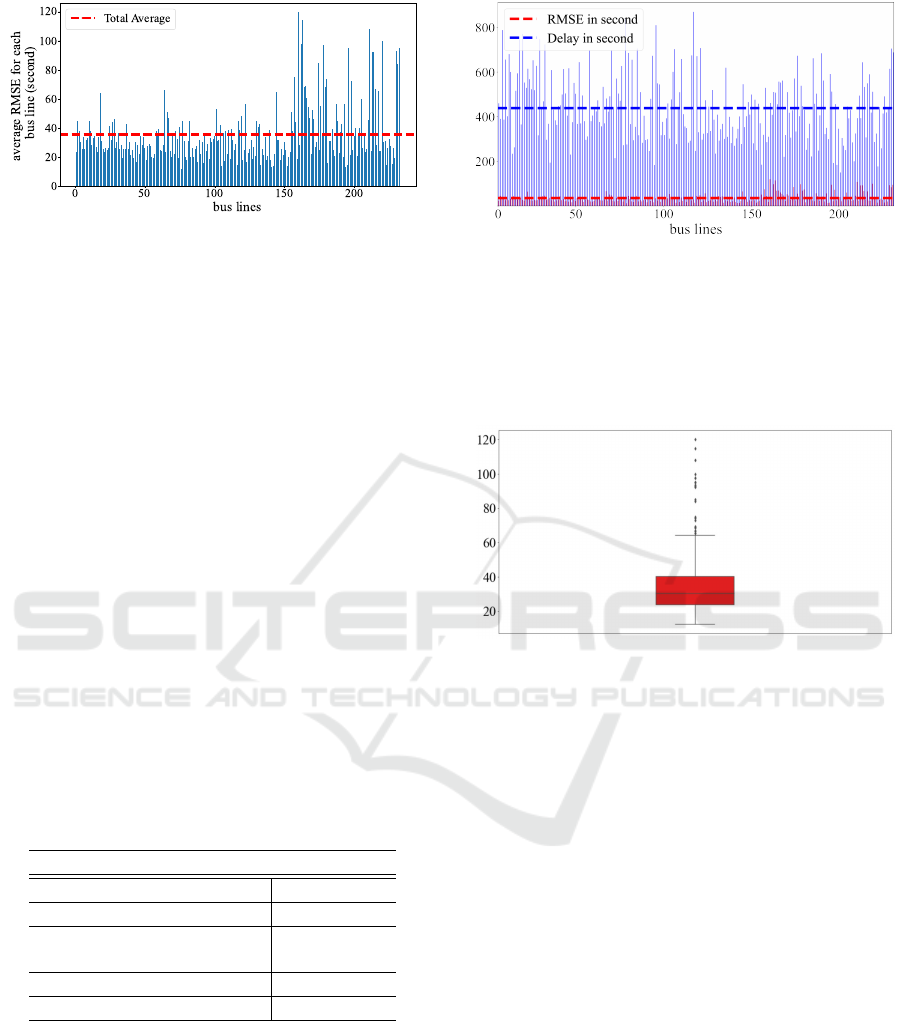
Figure 5: Performance of the model for all bus lines. The

average RMSE across all bus lines in the validation set is

35.74 seconds. Among the prediction error values, bus line

160 has the greatest RMSE, with a value of 119.99 seconds.

In contrast, the lowest error belongs to bus line 76 with an

RMSE equal to 12.42 seconds.

number 160, the lowest RMSE belongs to line num-

ber 76, with the RMSE equal to 12.42 seconds.

Additionally, Figure 6 illustrates the comparison

between the actual delay and RMSE of the predicted

arrival time across all bus lines in the validation set.

The large RMSE values in certain bus lines compared

to others could be due to the lack of relevant features

in predicting bus trip time. There is a wide range of

other factors affecting the bus trip time, but not avail-

able in this dataset. For instance, passenger demand is

a feature that this dataset does not include. By equip-

ping buses with passenger counting systems, passen-

ger demand for each bus stop can also be recorded.

This parameter impacts the bus dwell time, referring

to a bus’s time at a stop without moving. Addition-

ally, a potential area for future research could involve

investigating how weather types can inﬂuence error

arrival time prediction.

Table 4: Properties of the proposed model for bus arrival

time prediction on the New York dataset.

Model Properties

Total Training Time 7171s

Total Inference Time 2.42s

Inference Time per each

Validation Sample

0.00578 ms

Number of Parameters 164710

Computational Complexity 165380 Mac

In Figure 7, we have also shown RMSE distribu-

tion. Training time and inference time per each vali-

dation set data point are also presented in Table 4. The

average inference time for each validation data point

is 0.00578 ms. This implies if a passenger sends a re-

quest to the cloud to get the bus arrival time for their

trip, it takes less than 0.006 ms to produce AI-based

predictions. It should be noted this inference time in-

dicates the required time only for one access. When

Figure 6: Comparison between actual delay and RMSE

across validation set samples, containing 426,323 samples.

The average delay for all bus lines in the validation set is

438 seconds, while the prediction error over these samples

is less than 36 seconds.

thousands of passengers request bus arrival time to the

cloud, it will grow signiﬁcantly.

Figure 7: RMSE distribution in the form of a boxplot. It

displays the difference in RMSE values by showing the me-

dian of 35.74 seconds.

5.2.2 Scalability Comparison Between our

Model and SVR

Since there are more than 200 lines in the dataset,

a generalized model is needed to predict the arrival

time with the lowest possible error for all bus lines.

This section illustrates the scalability comparison of

our model and SVR for this dataset. The reason for

making this comparison is that SVR is among the

other machine learning approaches that are popular

for bus arrival time prediction problems, and a lot of

researchers used SVR with the Radial Basis Function

(RBF) kernel for bus arrival time prediction (Noor

et al., 2020).

So, for a different number of bus lines, SVR with

RBF kernel was used. The experimental results, as

observed in Figure 8, indicate that in a small number

of lines, SVR and our model prediction patterns are

almost the same. RMSE for prediction on 10 lines

using FCNN and SVR is 22.84 and 26.67, respec-

tively. When the number of lines rises from 10 to 20,

RMSE is 24.90 and 33.98, showing a notable increase

ICORES 2024 - 13th International Conference on Operations Research and Enterprise Systems

130

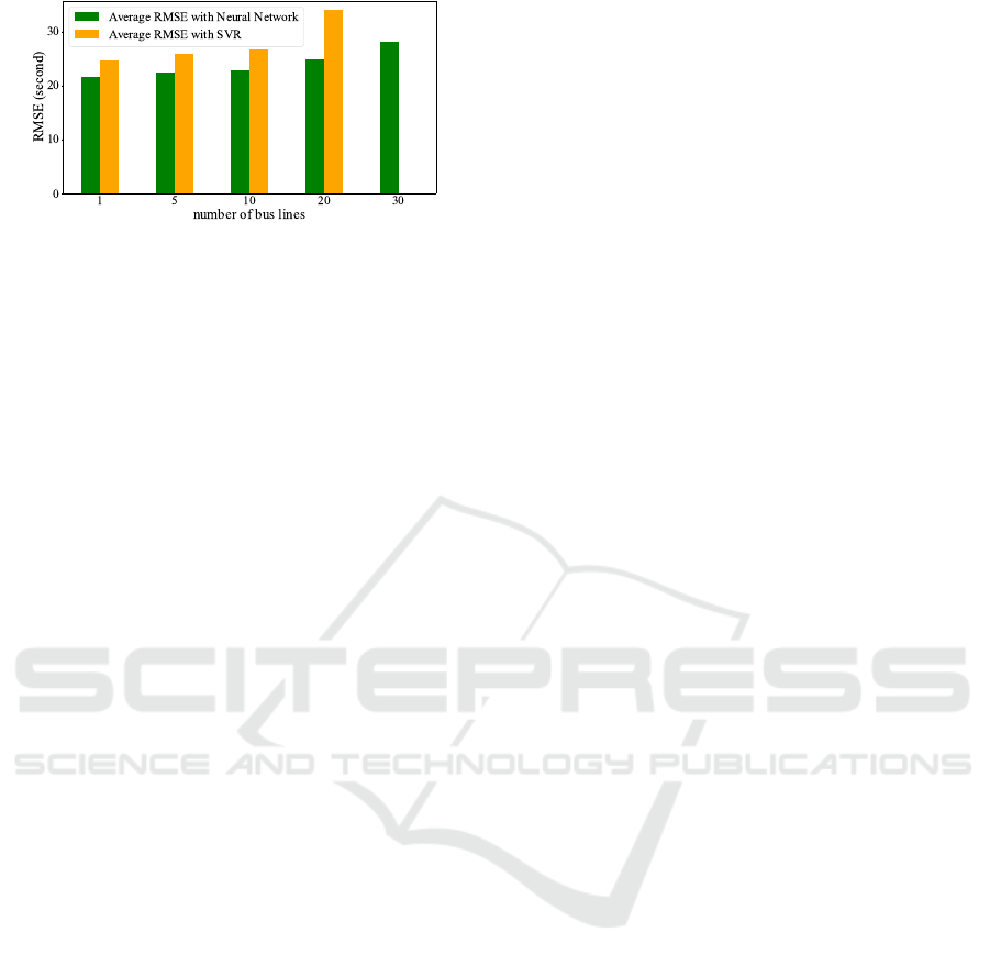
Figure 8: Scalability comparison of FCNN and SVR. These

two models were evaluated for different numbers of bus

lines. In the range of 1 to 20 bus lines, the accuracy of SVR

prediction decreased signiﬁcantly, while NN performance

remained almost unchanged. When the number of bus lines

exceeds 30, SVR can not be trained on this dataset.

in RMSE for the SVR model, and when the number of

bus lines surpasses 30, SVR becomes untrainable on

this dataset. Hence, in terms of scalability, our model

has a better prediction ability than SVR, which is why

FCNN was selected for the whole dataset.

6 CONCLUSIONS AND FUTURE

WORK

In this study, we engineered an AI-driven predic-

tion model aimed at propelling bus transit systems

into a realm of enhanced intelligence, thereby sig-

niﬁcantly elevating passenger experience by curtail-

ing protracted wait times. Our innovative blueprint

unfolds a real-time bus arrival prediction mechanism,

presenting a stark contrast to the conventional rigidity

of ﬁxed schedules.

The predictive model assimilates various input

features encompassing bus lines, distance, day type,

rush hour status, bus stops, and far status. The culmi-

nation of our endeavor, rooted in the Fully Connected

Neural Networks (FCNNs) framework, manifested in

an average estimated error reduction to less than 40

seconds across all bus lines within the dataset. This

outcome heralds a substantial leap forward when jux-

taposed against the average delay time embedded in

the dataset. Our forthcoming stride is geared towards

melding this AI-centric model within a smart mobile

application, thereby furnishing real-time insights to

commuters on the go.

The scope of this paper was partially tethered to

select features pertinent to bus trip time, dictated by

the constraints inherent in the utilized dataset. As

we move forward, numerous opportunities for future

research in this domain beckon exploration. Firstly,

investigating the integration of other factors, such

as passenger ﬂow, and meteorological conditions,

could provide a more comprehensive understanding

of the factors inﬂuencing bus arrival times. Addi-

tionally, delving into alternative architectures, partic-

ularly self-attention based neural networks, could en-

hance the model’s adaptability to diverse transporta-

tion datasets. The innate capacity of such models to

capture long-term temporal dependencies within the

bus data suggests their potential for having more ac-

curate and efﬁcient forecasting techniques in trans-

portation systems.

ACKNOWLEDGEMENT

This research is supported by the UNC Charlotte Col-

lege of Engineering seed grant and the UNC Charlotte

Urban Institute Urbain Institute for supporting this re-

search.

REFERENCES

(2017). New york city bus data.

(2017). Smart public transport – key to solving the urban

challenge - telia company. Accessed on Mar. 12, 2023.

(2019). Transport, data analytics and ai: Why tﬂ’s latest

initiative is good news. Accessed on Mar. 12, 2023.

(2022). September 2022 apta public transportation ridership

update. Accessed on Mar. 15, 2023.

(2023). Google maps vs waze – which one is better? Ac-

cessed on Mar. 15, 2023.

(2023). New york city transit key performance metrics. Ac-

cessed on Mar. 15, 2023.

Bai, C., Peng, Z.-R., Lu, Q.-C., and Sun, J. (2015). Dy-

namic bus travel time prediction models on road with

multiple bus routes. Computational intelligence and

neuroscience, 2015:63–63.

Chen, C., Chen, W., and Chen, Z. (2015). A multi-agent re-

inforcement learning approach for bus holding control

strategies. Advances in Transportation Studies.

Diab, E. I., Badami, M. G., and El-Geneidy, A. M. (2015).

Bus transit service reliability and improvement strate-

gies: Integrating the perspectives of passengers and

transit agencies in north america. Transport Reviews,

35(3):292–328.

Dubey, A. D., Basak, S. B., Sengupta, S. S., and Sun,

F. S. (2019). Data-driven optimization of public transit

schedule.

Erhardt, G. D., Hoque, J. M., Goyal, V., Berrebi, S., Brake-

wood, C., and Watkins, K. E. (2022). Why has

public transit ridership declined in the united states?

Transportation research part A: policy and practice,

161:68–87.

Freemark, Y. (2021). Us public transit has struggled to re-

tain riders over the past half century. reversing this

trend could advance equity and sustainability. urban

institute. The Urban Institute.

Real-Time Bus Arrival Prediction: A Deep Learning Approach for Enhanced Urban Mobility

131

Fu, J., Wang, L., Pan, M., Zuo, Z., and Yang, Q. (2014). Bus

arrival time prediction and release: system, database

and android application design. In International Con-

ference on Algorithms and Architectures for Parallel

Processing, pages 404–416. Springer.

Gaikwad, N. and Varma, S. (2019). Performance anal-

ysis of bus arrival time prediction using machine

learning based ensemble technique. In Proceedings

2019: Conference on Technologies for Future Cities

(CTFC).

Gholami, S., Lim, J. I., Leng, T., Ong, S. S. Y., Thompson,

A. C., and Alam, M. N. (2023). Federated learning for

diagnosis of age-related macular degeneration. Fron-

tiers in Medicine, 10.

Graehler, M., Mucci, R. A., and Erhardt, G. D. (2019).

Understanding the recent transit ridership decline in

major us cities: Service cuts or emerging modes. In

98th Annual Meeting of the Transportation Research

Board, Washington, DC.

Huang, H., Huang, L., Song, R., Jiao, F., and Ai, T.

(2022). Bus single-trip time prediction based on en-

semble learning. Computational intelligence and neu-

roscience, 2022.

Mallett, W. J. (2022). Public transportation ridership: Im-

plications of recent trends for federal policy. Technical

report.

Nannapaneni, S. and Dubey, A. (2019). Towards demand-

oriented ﬂexible rerouting of public transit under un-

certainty. In Proceedings of the Fourth Workshop on

International Science of Smart City Operations and

Platforms Engineering, pages 35–40.

Noghre, G. A., Katariya, V., Pazho, A. D., Neff, C., and

Tabkhi, H. (2022). Pishgu: Universal path prediction

architecture through graph isomorphism and attentive

convolution. arXiv preprint arXiv:2210.08057.

Noor, R. M., Yik, N. S., Kolandaisamy, R., Ahmedy, I.,

Hossain, M. A., Yau, K.-L. A., Shah, W. M., and

Nandy, T. (2020). Predict arrival time by using ma-

chine learning algorithm to promote utilization of ur-

ban smart bus.

Pandey, A., Lehe, L., and Monzer, D. (2021). Distributions

of bus stop spacings in the united states. Findings.

Pazho, A. D., Neff, C., Noghre, G. A., Ardabili, B. R.,

Yao, S., Baharani, M., and Tabkhi, H. (2023). Ancilia:

Scalable intelligent video surveillance for the artiﬁcial

intelligence of things. IEEE Internet of Things Jour-

nal.

Pulugurtha, S. S., Mishra, R., and Jayanthi, S. L. (2022).

Does transit service reliability inﬂuence ridership?

Sen, R., Bharati, A. K., Khaleghian, S., Ghosal, M., Wilbur,

M., Tran, T., Pugliese, P., Sartipi, M., Neema, H., and

Dubey, A. (2022). E-transit-bench: simulation plat-

form for analyzing electric public transit bus ﬂeet op-

erations. In Proceedings of the Thirteenth ACM In-

ternational Conference on Future Energy Systems (e-

Energy 2022).

Sun, F., Dubey, A., White, J., and Gokhale, A. (2019).

Transit-hub: A smart public transportation decision

support system with multi-timescale analytical ser-

vices. Cluster Computing, 22:2239–2254.

Sun, F., Pan, Y., White, J., and Dubey, A. (2016). Real-time

and predictive analytics for smart public transporta-

tion decision support system. In 2016 IEEE Inter-

national Conference on Smart Computing (SMART-

COMP), pages 1–8. IEEE.

Xu, H. and Ying, J. (2017). Bus arrival time prediction

with real-time and historic data. Cluster Computing,

20:3099–3106.

Yin, T., Zhong, G., Zhang, J., He, S., and Ran, B.

(2017). A prediction model of bus arrival time at stops

with multi-routes. Transportation research procedia,

25:4623–4636.

Zhong, G., Yin, T., Li, L., Zhang, J., Zhang, H., and Ran,

B. (2020). Bus travel time prediction based on ensem-

ble learning methods. IEEE Intelligent Transportation

Systems Magazine, 14(2):174–189.

ICORES 2024 - 13th International Conference on Operations Research and Enterprise Systems

132