Image Edge Enhancement for Effective Image Classification
Bu Tianhao
1
, Michalis Lazarou
2
and Tania Stathaki
2
1
Glory Engineering & Tech Co., LTD, China
2
Imperial College London, U.K.
Keywords:
Data Augmentation, Image Classification, High Boost Filtering, Edge Enhancement.
Abstract:
Image classification has been a popular task due to its feasibility in real-world applications. Training neural
networks by feeding them RGB images has demonstrated success over it. Nevertheless, improving the classi-
fication accuracy and computational efficiency of this process continues to present challenges that researchers
are actively addressing. A widely popular embraced method to improve the classification performance of
neural networks is to incorporate data augmentations during the training process. Data augmentations are
simple transformations that create slightly modified versions of the training data, and can be very effective
in training neural networks to mitigate overfitting and improve their accuracy performance. In this study, we
draw inspiration from high-boost image filtering and propose an edge enhancement-based method as means to
enhance both accuracy and training speed of neural networks. Specifically, our approach involves extracting
high frequency features, such as edges, from images within the available dataset and fusing them with the
original images, to generate new, enriched images. Our comprehensive experiments, conducted on two dis-
tinct datasets—CIFAR10 and CALTECH101, and three different network architectures—ResNet-18 ,LeNet-5
and CNN-9—demonstrate the effectiveness of our proposed method.
1 INTRODUCTION
Deep learning has undeniably been at the forefront of
technological advancement over the past decade, with
a transformative influence, particularly in the field of
computer vision (He et al., 2016). However, training
neural networks effectively for computer vision tasks
poses many limitations, because of the reliance on
substantial amount of data to avoid overfitting(Zhang
et al., 2019).
Data augmentation is a widely recognized tech-
nique for mitigating model overfitting and enhancing
generalization, effectively addressing the issue of in-
sufficient sample diversity(Shao et al., 2023). A com-
mon practice within the realm of data augmentation
is to apply colour space and/or other geometric trans-
formations to the original images in order to increase
the size and diversity of the training dataset. Some
notable works of data augmentation techniques in-
clude image mix-up approaches, such as the creation
of new images by directly merging two images from
distinct classes (Zhang et al., 2017), replacing specific
regions of an image with patches from other images
(Yun et al., 2019) and various other inventive varia-
tions (Liu et al., 2022), (Yin et al., 2021), (Kim et al.,
2020). Other approaches utilize the frequency domain
information (Chen and Wang, 2021), (Mukai et al.,
2022) with a focus on generating new sets of images
from diverse sources.
In our work, we present a novel data augmentation
method that transforms the original images by merg-
ing them with their corresponding extracted edges,
that we will refer to as Edge Enhancement (E
2
). It
operates on the same principle as high boost image
filtering, a technique that accentuates the edges of
an image without completely eliminating the back-
ground. The proposed E
2
method extracts the edges
(high frequency components) from each of the RGB
channels of the original images and subsequently in-
tegrates these extracted features with the original im-
age to yield the edge-enhanced images. E
2
adheres to
the fundamental concept of introducing subtle modi-
fications by utilizing these extracted features to gen-
erate new images, all without relying on complex al-
gorithms, thus ensuring efficient preprocessing.
The main contributions of our work are summa-
rized as follows:
1. We propose a novel data augmentation method
that enhances the semantic information of every
image in the training dataset which in turn im-
proves the training of neural networks.
2. Our method has undergone rigorous evaluation
on two distinct datasets, CIFAR10 and CAL-
TECH101, employing neural network models in-
444
Tianhao, B., Lazarou, M. and Stathaki, T.
Image Edge Enhancement for Effective Image Classification.
DOI: 10.5220/0012364900003660
Paper published under CC license (CC BY-NC-ND 4.0)
In Proceedings of the 19th International Joint Conference on Computer Vision, Imaging and Computer Graphics Theory and Applications (VISIGRAPP 2024) - Volume 3: VISAPP, pages
444-451
ISBN: 978-989-758-679-8; ISSN: 2184-4321
Proceedings Copyright © 2024 by SCITEPRESS – Science and Technology Publications, Lda.

Figure 1: Edge enhancement process. Leftmost: original image. Mid left: corresponding R,G,B channels of the original
labelled data. Mid right:corresponding extracted edges Rightmost: edge enhanced image.
cluding CNN-9, LeNet-5 and RESNET-18. These
experiments have consistently showcased sub-
stantial improvements in classification accuracy,
accompanied by a reduced requirement for train-
ing epochs to achieve optimal classification accu-
racy.
2 BACKGROUND
2.1 Data Augmentation
Data augmentation is a technique that expands dataset
sizes by introducing subtle alterations.
The simplest data augmentation strategies are
through applying geometric transformations as rota-
tion and flipping (Chlap et al., 2021). Our research
aligns with this principle of generating new labeled
data by modifying the original dataset. However, it
deviates from the conventional methods of rotation
and flipping. Instead, we propose a novel approach
that prioritizes the enhancement of semantic informa-
tion. This innovative method draws inspiration from
the concept of high-boost filtering, which will be elab-
orated upon in the subsequent section.
2.2 High Boost Filtering
High-boost filtering is a well-established image pro-
cessing technique, representing a variation of high-
pass filtering. In contrast to high-pass filtering, high-
boost filtering aims to accentuate an image’s high-
frequency information while preserving the back-
ground. Let’s denote an image undergoing this pro-
cess as I(u,v) (Srivastava et al., 2009), where u,v cor-
respond to spatial coordinates. High boost filtering
can be formally defined as follows:
I
boost
(u,v) = A · I(u,v) − I
low
(u,v) (1)
where I
boost
(u,v) is the high boosted image pixel
at location u, v, and A is a scaling factor greater than
1 (common choices are 1.15, 1.2) and I
low
(u,v) is the
low pass filtered image pixel. Respectively, the high
pass filtering can be presented in a similar way as,
I
high
(u,v) = I(u,v) − I
low
(u,v) (2)
where I
high
(u,v) is the high pass filtered image pixel
at location u, v. Our method employs the concept of
high-boost filtering, where we combine the high-pass
filtered image with the original version, with A = 2.
This selection for A can be viewed as a particular in-
stance of high-boost filtering.
2.3 Canny Edge Detection
Canny edge detection algorithm was invented by John
F Canny in 1986 (Canny, 1986). The procedure of
canny edge detection can be shown as follows: 1)
Noise suppression within the image is accomplished
by employing a Gaussian filter (a low-pass filter)
(Deng and Cahill, 1993). The kernel for the 2-D
Gaussian filter can be represented as:
G(u,v) =
1
2πσ
2
e
−
u
2
+v
2
2σ
2
(3)
The denoised result is achieved by convolving the ker-
nel with the image, where σ
2
represents the filter vari-
ance. 2) Determine the edge strength ∇G and the four
orientations θ (horizontal, vertical and the two diago-
nals), expressed as
∇G = (
∂G
∂u
+
∂G
∂v
)
0.5
(4)
θ = tan
−1
(
∂G
∂v
/
∂G
∂u
) (5)
where
∂G
∂u
,
∂G
∂v
are the first order derivatives (gradi-
ents) in the horizontal and vertical directions. 3)
Non-maximum suppression, which utilizes the edge
strength to suppress non-edge pixels. 4) Double
thresholding, a method which involves establishing
both high and low edge strength thresholds, which
Image Edge Enhancement for Effective Image Classification
445

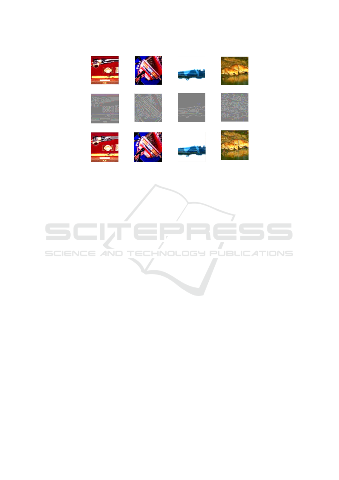
Figure 2: A batch of 4 images. Top row: original data. Mid row: corresponding extracted edges. Bottom row: corresponding
edge enhanced data.
are employed to categorize the strength of edge pix-
els into three levels: strong, weak, and non-edges.
Additionally, non-edge pixels are subsequently sup-
pressed. 5) Hysteresis edge tracking represents the
final step, employing blob analysis to further han-
dle weak edges. Those weak edges which lack a
strong edge neighbor connection are identified as po-
tential noise or color variation-induced edges and sub-
sequently removed. In our work we use Canny edge
detection as a core technique to extract the edge in-
formation in each colour channel from the dataset of
interest.
3 METHODOLOGY
3.1 Problem Definition
Let us define a labeled image dataset D = (x
i
,y
i
),
where x
i
represents the i
th
image and y
i
represents
the corresponding class label of image x
i
.This dataset
comprises the images, each containing three RGB
channels. The dataset is partitioned into three splits:
the training set split, D
train
= (x
i
,y
i
), the valida-
tion set split, D
val
= (x
i
,y
i
) and testing set split,
D
test
= (x
i
,y
i
). We use D
train
to train a neural net-
work, that consists of a backbone f
θ
and a classifier
g
φ
(last layer of the network). Additionally, we denote
the edge features extracted from the training data as
v
i
, this is merged with x
i
to create the edge enhanced
data e
i
.
The validation set D
val
is used in order to save the
model with the highest validation accuracy. Finally,
we use D
test
to calculate the test set classification ac-
curacy.
3.2 Edge Enhancement
Our E
2
pre-processing can be illustrated in Figure 1,
where the leftmost image is the original data. Af-
ter applying Canny filtering the extracted edges are
shown and the rightmost image is the edge enhanced
result. We first apply normalization to the sample
images, and then resize the images to ensure all im-
ages have exactly the same resolution, also maintain-
ing consistent image size across the datasets. Canny
filters are employed to the every image at each of its
RGB channels to obtain the extracted edge informa-
tion. The extracted edge information is then com-
bined with their respective original versions, resulting
in a transformed image set. Each image in this set is
labeled according to the original class labels.
3.3 Training Phase
In each batch, we apply edge enhancement to a set
of training images, as depicted in Figure 2. In
this representation, the top four images represent the
original data, while the bottom four belong to the
edge-enhanced images, corresponding to the edge-
enhanced dataset
e
D =
e
x,
e
y, where
e
x is the edge-
enhanced image and
e
y is the corresponding class label
of image
e
x. These edge-enhanced images are com-
bined with the original training set images to create
the input data for the network model. Consequently,
each batch sample comprises a total of eight images,
contributing to the generation of classification results.
During the forward propagation, we extract the
features v
i
by inputting every image x
i
into the Canny
edge detection function, denoted as Canny(). These
VISAPP 2024 - 19th International Conference on Computer Vision Theory and Applications
446

Original data
Original data
+
Edge enhanced data
Edge Enhancement
Training
+
Classification
Classification results
class 1
class 2
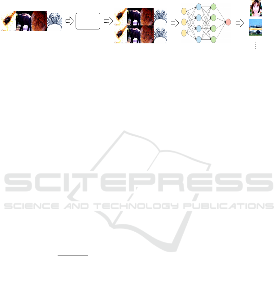
Figure 3: The flowchart of the edge enhancement method for model training. i) Original data is edge enhanced to the
transformed data. ii) The original and transformed data is concatenated then feed into the network. iii) Model training. iv)
Classification results obtained through test dataset.
features can be expressed as follows:
e
x
i
:= Canny(x
i
) + x
i
(6)
During the training phase, the edge-enhanced and
original images are both used to train the network by
concatenating them together before feeding them to
the network. Therefore, every batch size now con-
tains both the edge enhanced images, {
e
x
i
}
b
i=1
, and the
original images, {x
i
}
b
i=1
, where b represents the batch
size. After, the concatenation we have {u
i
}
2b
i=1
be-
cause the size of the new batch size is 2b. We feed
every image u
i
from the new batch to network f
θ
to
obtain the feature vector z
i
that corresponds to image
u
i
, expressed as
z
i
:= f
θ
(u
i
)
(7)
We pass z
i
to g
φ
so that
c
i
:= g
φ
(z
i
) (8)
where c
i
is the vector of logits of image i. We obtain
the probability of each class ˆp
i
by using the softmax
activation function
ˆp
i
:=
exp(c
i
)
∑
N
i=1
exp(c
i
)
, (9)
where N is the total number of classes. With the aid of
equation (9), we calculate the cross-entropy loss L
ce
as
L
ce
:= −
∑
i∈N
y
i
log( ˆp
i
), (10)
where y
i
represents the one hot encoded version of y
i
.
Back propagation is then performed to calculate the
gradient of L
ce
with respect to the network weight.
Algorithm 1 summarizes the training procedure of
E
2
, and the corresponding flowchart is illustrated in
Figure 3
3.4 Inference Stage
During the inference stage, we calculate the proba-
bility vector, ˆp
i
, for each image x
i
in the test dataset,
D
test
by embedding image x
i
using the functions f
θ
,
g
φ
and equation (9). To predict the class label
ˆ
y
i
of
image x
i
we employ the following formula:
ˆ
y
i
:= arg max
j∈[N]
ˆp
i j
(11)
where N is the number of possible classes and the re-
sult corresponds to the position of the element with
the highest class probability in the class probability
vector p
i
.
We calculate the test dataset accuracy using the
following formula:
S
c
:= Acc(y
i
,
ˆ
y
i
) (12)
where S
c
is the overall classification accuracy, and
Acc is the accuracy function that sums up the numbers
of correct comparison results between the prediction
and true class labels, we denote the sum as N
correct
. To
scale them into percentage, the results are divided by
total number of images and multiplied by a hundred,
we express it as
N
correct
N
total
× 100.
4 EXPERIMENTS
4.1 Setup
Datasets. In our experiments two datasets are used:
1) CIFAR10, which is one of the most popular data
sets in image classification research (Recht et al.,
2018). It contains a total of 60000 color images of
10 classes, each with dimensions of 32 by 32 pixels.
In our experiment we use 45000 images for training,
5000 images for validation and 10000 for testing.
2) CALTECH101, considered as one of the challeng-
ing datasets (Bansal et al., 2021), CALTECH101 fea-
tures higher resolution images in comparison to CI-
FAR10, as depicted in Figure 1,Figure 2, and Fig-
ure 3. This dataset contains 101 classes and includes
8,677 images. For consistency in feeding images into
the networks, we resized each image to 256 by 256
pixels and then center-cropped them to 224 by 224
Image Edge Enhancement for Effective Image Classification
447

Algorithm 1: Edge enhancement training procedure.
input : training dataset D
train
= x
i
,y
i
output : trained neural network model
1
batch size: 4; if D
train
∈ CALTECH101 then
2 D
train
= Resize(D
train
, 256 x 256),
3 D
train
= CenterCrop(D
train
, 224 x 224)
4 D
train
= Normalization( D
train
) while epoch not
finished do
5 for i <= D
train
.size() do
6 feature = Canny(x
i
,sigma = 3),
7
e
x
i
= add(x
i
,feature),
8 Inputs = concat(x
i
,
e
x
i
)
9 Model = Model.train(Inputs, D
val
)
pixels. Out of these images, 5,205 were used in the
training set, 579 for validation, and 2,893 for testing.
Implementation Details. Our implementation is
based in Python. We utilized the skimage package
for the Canny edge detector and Pytorch for training
our neural networks.
Networks. In our work, we used three differ-
ent neural network architectures tailored to the two
datasets to investigate the robustness of our method
with different networks and datasets. 1) LeNet-5:
This convolutional neural network (CNN) originally
proposed by LeCun in 1998(lec, 1998), was ini-
tially designed for hand written character classifica-
tion. Given its compatibility with 32 by 32 pixel im-
ages and suitability for datasets with small class sizes
(10 in CIFAR10), we selected this network for the CI-
FAR10 dataset, due to its nature of accepting 32 by
32 images and suitable for small class sizes (10 for
CIFAR10). 2) CNN-9: A standard neural network
model with six convolutional layers and three linear
layers, again suitable for 32 by 32 images. 3) ResNet-
18: This network, proposed by (He et al., 2016) in
2016. It is designed for larger images of size 224
by 224 pixels. We used this network for the high-
resolution CALTECH101 dataset after preprocessing
the data to meet the network’s input requirements.
Hyperparameters. In the experiment, the batch
size is fixed at 4, meaning 4 labeled images were en-
hanced with edge information simultaneously. We set
the standard deviation σ of the Canny edge detector to
3 and trained the CIFAR10 dataset with LeNet-5 and
CNN-9 for 50 epochs. For the CALTECH101 dataset,
we trained ResNet-18 for 100 epochs. The loss func-
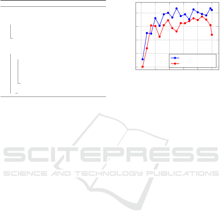
0 10 20 30 40 50
55
60
65
70
75
Epochs
validation accuracy
edge-enhancement
original
Figure 4: CIFAR10 through CNN-9.
tion used is the cross-entropy loss due to its strong
performance in multi-class classification tasks.(Zhou
et al., 2019). For weight optimization during network
training, we used Stochastic Gradient Descent (SGD)
with a momentum of 0.9, weight decay of 0.0005, and
learning rate of 0.01. We use the validation set to cal-
culate the validation accuracy and save the model with
the highest validation accuracy through comparisons
at each epoch.
4.2 Ablation Study
In our experimental setup, for each training dataset
and network architecture, we compared our edge en-
hancement method with the baseline method, which
involved training on the original data without any
modifications. We assessed this comparison through
two aspects: 1) Validation Accuracy Variation: We
monitored the validation accuracies for both meth-
ods throughout the training process, recording them
at each epoch and presenting the results in graph-
ical form. 2) Testing Accuracy: After identifying
the models that achieved the best validation results,
we tested them on the respective testing datasets to
obtain optimal classification accuracies, which were
then presented in a tabular format.
1) CIFAR10: Figure 4 and Figure 5 display the results
obtained from both LeNet-5 and CNN-9 networks.
In these figures, the edge enhancement method is
represented by the blue lines, and it consistently
outperforms the original method indicated by the
red lines. The validation accuracy of the edge en-
hancement method surpasses that of the original at
nearly every epoch. Under LeNet-5, the edge en-
hancement method achieves its highest accuracy at
55.74%, differing from its lowest accuracy (40.05%)
by a substantial 15.69%. In contrast, the original
VISAPP 2024 - 19th International Conference on Computer Vision Theory and Applications
448

method exhibits a maximum-minimum difference of
15.24%. Similarly, with CNN-9, the edge enhance-
ment method shows a maximum-minimum differ-
ence of 18.86%, compared to the original method’s
18.62%. These results clearly indicate that the edge
enhancement method consistently provides greater
accuracy improvement during the training process.
Furthermore, our results reveal a noteworthy trend:
for both network architectures within the CIFAR10
dataset, the validation accuracy variations are notably
more stable and compact when using the edge en-
hancement method. CALTECH101: In Figure 6,
we present the results obtained through ResNet-18.
Here, the edge enhancement method demonstrates a
maximum-minimum difference of 44.73%, while the
original method yields a value of 40.61%. Once
again, these findings underscore the effectiveness of
our method in achieving more substantial accuracy
improvements.
2) In Table 1, we present the testing accuracy results,
where E
2
denotes the edge enhancement method, and
’epoch’ indicates the epoch at which the optimal
model was achieved. CIFAR10: For the CIFAR10
dataset employing LeNet-5, our method stands out
with an impressive 5.7% increase in accuracy over the
original approach. Moreover, it achieves this remark-
able performance while converging 12 epochs faster
to reach an optimal model. In the case of CNN-9 ap-
plied to CIFAR10, our method still shines, delivering
a substantial 4.03% accuracy improvement. Notably,
it accomplishes this while requiring 18 fewer epochs
to converge. These outcomes underscore the signif-
icant enhancements our method brings to both net-
work architectures when working with the CIFAR10
dataset.
CALTECH101: Through ResNet-18, our method
demonstrated a 1.56% improvement over the original
method, required 30 less epochs to converge. To con-
clude, the experiment results are sufficient to show
that the proposed edge enhancement method for neu-
ral network training provide noticeable classification
accuracy improvement and it is more computationally
efficient.
4.3 Comparisons with Transformation
Methods
To further investigate the effectiveness of our edge en-
hancement method, we conducted a comprehensive
evaluation by integrating it with various geometric
transformation techniques. Specifically, we assessed
its performance in combination with transformations
like random horizontal flipping and random image
size cropping. Our objective was to compare the out-
comes with a baseline approach that underwent the
same corresponding transformations. We refer to the
use of Random Cropping as C and Random Flipping
as F.
In this experiment, we use the pytorch built-in
transform functions and we split the comparisons
within each dataset into three types: 1. exclusively
applying random horizontal flipping. 2. solely im-
plementing random image cropping . 3. simultane-
ously employing both random flipping and random
cropping. The image classification accuracy results
specified to each dataset section are compared, along
with the results obtained without any geometric trans-
formations, as shown in Table 1.
Random Horizontal Flip. The "random horizontal
flip" operation involves flipping the input data hori-
zontally with a specified probability. In our experi-
ment, we maintained a default probability of 50 per-
cent for applying this random flipping to the input
data.
Random Image Crop. The "random image crop"
operation involves selecting a random location within
the given input data and then resizing the cropped por-
tion to a specified size. In our experiment, we adapted
the resizing process based on the dataset being used:
for CIFAR10, we resize the cropped data to 32 by 32
matching the original data size, suitable for LeNet-5
and CNN-9; for CALTECH101, since we use ResNet-
18 for this data set, we again resize the cropped data
to 224 by 224 fitting the requirement.
As the results shown in Table 2, when applied
to the CIFAR10 dataset with network LeNet-5 our
edge enhancement method provides significant ac-
curacy improvements over the baseline under every
transformation scenario. These improvements range
from 3.16% to 3.97% when compared to the base-
line. Notably, even when combined with random flip-
ping, our method performs just 0.32% worse than
our method without any transformations, as detailed
in Table 1. Turning our attention to the Caltech101
dataset with ResNet-18, Table 3 showcases a sim-
ilar trend. Our edge enhancement method consis-
tently outperforms the original approach for all se-
lected transformation combinations, with improve-
ments ranging from 0.96% to 1.97%. In this case,
both edge enhancement with random cropping and
edge enhancement with both cropping and flipping
surpass the unmodified method (with no transforma-
tions) from Table 1 in terms of performance. Further-
more, when considering the impact of these transfor-
Image Edge Enhancement for Effective Image Classification
449

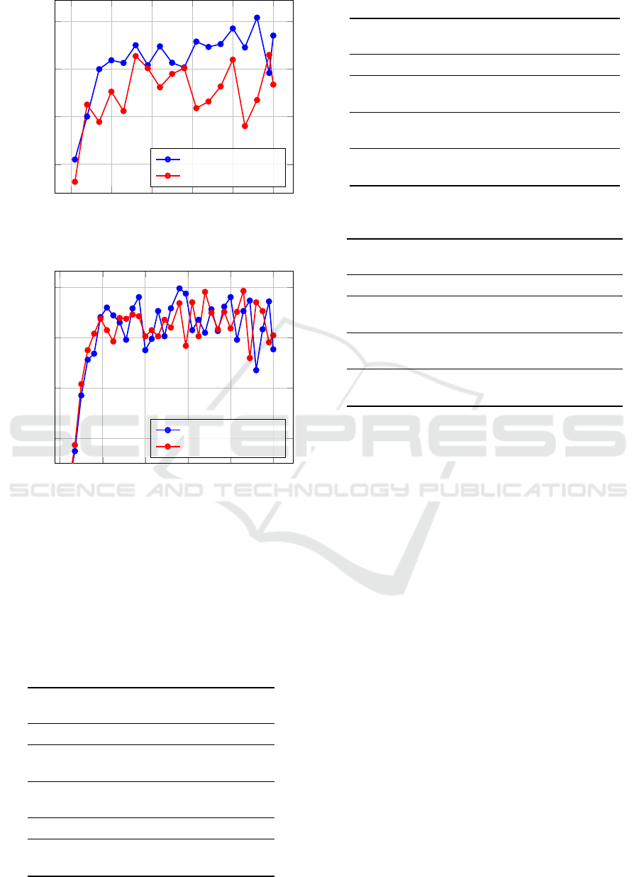
0 10 20 30 40 50
40
45
50
55
Epochs
validation accuracy
edge-enhancement
original
Figure 5: CIFAR10 through LeNet-5.
0 20 40 60 80 100
40
50
60
70
Epochs
validation accuracy
edge-enhancement
original
Figure 6: CALTECH101 through ResNet-18.
mation techniques, our results affirm the claim that
edge enhancement substantially enhances image clas-
sification accuracy. Intriguingly, for both datasets us-
ing LeNet-5 and ResNet-18, the original method with
random cropping and flipping demonstrates a faster
convergence to optimal performance compared to all
other results.
Table 1: Testing accuracy results.
METHOD
backbone accuracy% epoch
CIFAR10
Original LeNet-5 49.26 45
E
2
LeNet-5 54.96 33
Original CNN-9 72.61 43
E
2
CNN-9 76.64 25
CALTECH101
Original ResNet-18 72.83 86
E
2
ResNet-18 74.39 56
Table 2: CIFAR10 transformation testing accuracy results.
METHOD
backbone accuracy% epoch
CIFAR10
Original + F LeNet-5 50.67 45
E
2
+ F LeNet-5 54.64 32
Original + C LeNet-5 46.74 29
E
2
+ C LeNet-5 49.90 17
Original + F+C LeNet-5 44.59 16
E
2
+ F+C LeNet-5 48.54 49
Table 3: CALTECH101 transformation testing accuracy re-
sults.
METHOD
backbone accuracy% epoch
CALTECH101
Original + F ResNet-18 71.00 80
E
2
+ F ResNet-18 71.96 53
Original + C ResNet-18 79.23 88
E
2
+ C ResNet-18 81.20 58
Original + C+F ResNet-18 78.40 89
E
2
+ F+C ResNet-18 79.81 92
5 CONCLUSION
In our research, we introduced a novel approach for
enhancing image classification accuracy and com-
putational efficiency. Our method, based on the
high boost filtering principle, focuses on edge en-
hancement. This technique leverages the edge infor-
mation from labeled data to transform the original
dataset, thereby increasing both the size and diver-
sity of the training samples. Through extensive ex-
periments on popular datasets such as CIFAR-10 and
CALTECH-101, using well-known neural network ar-
chitectures including LeNet-5, CNN-9, and ResNet-
18, we have demonstrated the effectiveness of our
proposed method. Our results substantiate the validity
of our hypothesis. Regarding our future research di-
rections, we are interested in exploring the impact of
data augmentation techniques in conjunction with our
current state-of-the-art approach; additionally, scal-
ing our method to larger datasets such as ImageNet
and other domains as semi-supervised learning would
be another potential research direction. Our goal is
to further enhance classification accuracy while at the
same time improving the training efficiency, pushing
the boundaries of what is achievable in image classi-
fication.
VISAPP 2024 - 19th International Conference on Computer Vision Theory and Applications
450

ACKNOWLEDGEMENTS
In the loving memory of TianHao Bu’s father
BingXin Bu: 10/01/1965 - 13/09/2023.
REFERENCES
(1998). Gradient-based learning applied to document recog-
nition. Proceedings of the IEEE, 86(11):2278–2324.
Bansal, M., Kumar, M., Sachdeva, M., and Mittal, A.
(2021). Transfer learning for image classification us-
ing vgg19: Caltech-101 image data set. Journal of
ambient intelligence and humanized computing, pages
1–12.
Canny, J. (1986). A computational approach to edge de-
tection. IEEE Transactions on pattern analysis and
machine intelligence, (6):679–698.
Chen, X. and Wang, G. (2021). Few-shot learning by inte-
grating spatial and frequency representation. In 2021
18th Conference on Robots and Vision (CRV), pages
49–56. IEEE.
Chlap, P., Min, H., Vandenberg, N., Dowling, J., Holloway,
L., and Haworth, A. (2021). A review of medical im-
age data augmentation techniques for deep learning
applications. Journal of Medical Imaging and Radia-
tion Oncology, 65(5):545–563.
Deng, G. and Cahill, L. (1993). An adaptive gaussian fil-
ter for noise reduction and edge detection. In 1993
IEEE conference record nuclear science symposium
and medical imaging conference, pages 1615–1619.
IEEE.
He, K., Zhang, X., Ren, S., and Sun, J. (2016). Deep resid-
ual learning for image recognition. In Proceedings of
the IEEE conference on computer vision and pattern
recognition, pages 770–778.
Kim, J.-H., Choo, W., and Song, H. O. (2020). Puzzle
mix: Exploiting saliency and local statistics for op-
timal mixup. In International Conference on Machine
Learning, pages 5275–5285. PMLR.
Liu, Z., Li, S., Wu, D., Liu, Z., Chen, Z., Wu, L., and Li,
S. Z. (2022). Automix: Unveiling the power of mixup
for stronger classifiers. In European Conference on
Computer Vision, pages 441–458. Springer.
Mukai, K., Kumano, S., and Yamasaki, T. (2022). Im-
proving robustness to out-of-distribution data by
frequency-based augmentation. In 2022 IEEE In-
ternational Conference on Image Processing (ICIP),
pages 3116–3120. IEEE.
Recht, B., Roelofs, R., Schmidt, L., and Shankar, V. (2018).
Do cifar-10 classifiers generalize to cifar-10? arXiv
preprint arXiv:1806.00451.
Shao, S., Wang, Y., Liu, B., Liu, W., Wang, Y., and Liu,
B. (2023). Fads: Fourier-augmentation based data-
shunting for few-shot classification. IEEE Transac-
tions on Circuits and Systems for Video Technology.
Srivastava, R., Gupta, J., Parthasarthy, H., and Srivastava,
S. (2009). Pde based unsharp masking, crispening
and high boost filtering of digital images. In Contem-
porary Computing: Second International Conference,
IC3 2009, Noida, India, August 17-19, 2009. Proceed-
ings 2, pages 8–13. Springer.
Yin, W., Wang, H., Qu, J., and Xiong, C. (2021). Batch-
mixup: Improving training by interpolating hidden
states of the entire mini-batch. In Findings of the Asso-
ciation for Computational Linguistics: ACL-IJCNLP
2021, pages 4908–4912.
Yun, S., Han, D., Oh, S. J., Chun, S., Choe, J., and Yoo,
Y. (2019). Cutmix: Regularization strategy to train
strong classifiers with localizable features. In Pro-
ceedings of the IEEE/CVF international conference
on computer vision, pages 6023–6032.
Zhang, H., Cisse, M., Dauphin, Y. N., and Lopez-Paz, D.
(2017). mixup: Beyond empirical risk minimization.
arXiv preprint arXiv:1710.09412.
Zhang, H., Zhang, L., and Jiang, Y. (2019). Overfitting
and underfitting analysis for deep learning based end-
to-end communication systems. In 2019 11th inter-
national conference on wireless communications and
signal processing (WCSP), pages 1–6. IEEE.
Zhou, Y., Wang, X., Zhang, M., Zhu, J., Zheng, R., and Wu,
Q. (2019). Mpce: a maximum probability based cross
entropy loss function for neural network classification.
IEEE Access, 7:146331–146341.
Image Edge Enhancement for Effective Image Classification
451