Assessing the Performance of Autoencoders for Particle Density

Estimation in Acoustoﬂuidic Medium: A Visual Analysis Approach

Lucas M. Massa

1 a

, Tiago F. Vieira

1 b

, Allan de M. Martins

2 c

and Bruno G. Ferreira

3 d

Institute of Computing, Federal University of Alagoas, Lourival Melo Mota Av., Macei

o, Brazil

Department of Electrical Engineering, Federal University of Rio Grande do Norte, Natal, Brazil

Edge Innovation Center, Federal University of Alagoas, Macei

o, Brazil

Keywords:

Particle Density Estimation, Convolutional Autoencoder, Particle Size Estimation, Acoustoﬂuidics.

Abstract:

Micro-particle density is important for understanding different cell types, their growth stages, and how they

respond to external stimuli. In previous work, a Gaussian curve ﬁtting method was used to estimate the

size of particles, in order to later calculate their density. This approach required a long processing time,

making the development of a Point of Care (PoC) device difﬁcult. Current work proposes the application

of a convolutional autoencoder (AE) to estimate single particle density, aiming to develop a PoC device that

overcomes the limitations presented in the previous study. Thus, we used the AE to bottleneck a set of particle

images into a single latent variable to evaluate its ability to represent the particle’s diameter. We employed

an identical physical apparatus involving a microscope to take pictures of particles in a liquid submitted to

ultrasonic waves before the settling process. The AE was initially trained with a set of images for calibration.

The acquired parameters were applied to the test set to estimate the velocity at which the particle falls within

the ultrasonic chamber. This velocity was later used to infer the particle density. Our results demonstrated that

the AE model performed much better, notably exhibiting signiﬁcantly enhanced computational speed while

concurrently achieving comparable error in density estimation.

1 INTRODUCTION

Density establishes a fundamental relationship be-

tween the mass and volume of a particle, thereby as-

sisting in the determination of cell types and their cor-

responding stage cycles (Bryan et al., 2010). Addi-

tionally, cell volume shows a direct correlation with

the mass and energy requirements of cell division. By

leveraging density measurements, it becomes possi-

ble to estimate ﬂuctuations in the volume of a cell. To

(Zhao et al., 2014), cell mass and density measure-

ments offer a powerful and direct method for monitor-

ing cellular responses to various external stimuli, such

as drug interventions and environmental changes.

On this basis, researchers across various scientiﬁc

areas have employed different methods to measure the

density of particles. In (Castiglioni et al., 2021), a

method is proposed to measure the density of porous

particles, speciﬁcally activated carbons, by measur-

https://orcid.org/0009-0001-6023-9318

https://orcid.org/0000-0002-5202-2477

https://orcid.org/0000-0002-9486-4509

https://orcid.org/0000-0003-1345-5103

ing the volume of pores using gas or solution expo-

sure. The work proposed by (Pl

uisch et al., 2021)

presents a microﬂuidic device to measure the den-

sity of single cells using a suspended microchannel

resonator (SMR). Some authors propose using cen-

trifuges (Minelli et al., 2018; Uttinger et al., 2020;

Ullmann et al., 2017; Maric et al., 1998) to obtain this

measurement. However, these methods have some

signiﬁcant downsides. While SMRs have a costly

and challenging fabrication process (De Pastina et al.,

2018), centrifuges may potentially damage the cells

under analysis.

There is a particularly interesting method based on

acoustoﬂuidics where the particle is placed inside a

resonant chamber containing a speciﬁc ﬂuid and sub-

mitted to an ultrasonic ﬁeld used for manipulation and

observation. This consists of a contactless, biocom-

patible approach and has been applied to different ar-

eas of science (Wu et al., 2019; Yazdani and S¸is¸man,

2020; Rasouli et al., 2023; Xie et al., 2019; Li and

Huang, 2018).

To the best of our knowledge, the most recent

work using computer vision in this context was in-

436

Massa, L., Vieira, T., Martins, A. and Ferreira, B.

Assessing the Performance of Autoencoders for Particle Density Estimation in Acoustoﬂuidic Medium: A Visual Analysis Approach.

DOI: 10.5220/0012364500003660

Paper published under CC license (CC BY-NC-ND 4.0)

In Proceedings of the 19th International Joint Conference on Computer Vision, Imaging and Computer Graphics Theory and Applications (VISIGRAPP 2024) - Volume 3: VISAPP, pages

436-443

ISBN: 978-989-758-679-8; ISSN: 2184-4321

2 - TRAINING

1 - PREPROCESSING

Resize

Contrast

Enhacement

PROPORTIONAL

TO PARTICLE

AREA

A1 A2 A3 A4 A5 A6

3 - INFERENCE

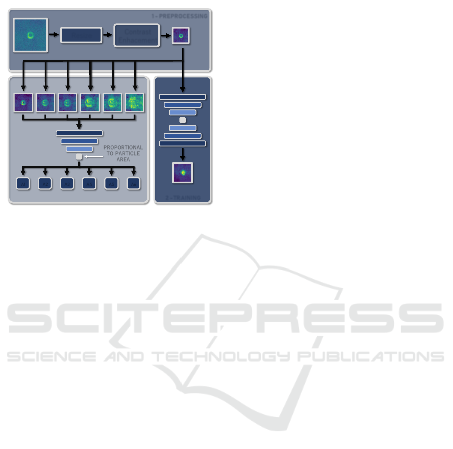
Figure 1: Overview of the proposed approach. Initially,

some particle images collected from a microscope were

used to train a convolutional autoencoder that squeezes a

single latent variable. Hypothetically, this value is expected

to be proportional to the particle area. Lastly, the values

returned by the encoder are used along with the calibration

curve and physical relationship to estimate the particle den-

sity.

troduced in (Massa et al., 2023), where they analyzed

microscopic images acquired during the settling pro-

cess within an acoustoﬂuidic medium. Their method

involves extracting particle areas by ﬁtting 2D Gaus-

sian functions to estimate particle size using a ge-

netic algorithm optimization. These extracted values

are subsequently employed to estimate the particle

fall velocity and its density. While the authors have

demonstrated promising outcomes, some aspects ne-

cessitate improvement. The primary concern is the

requirement of executing the genetic algorithm for ev-

ery new image along a given experiment. In contrast,

we propose using a machine learning pipeline, which

allows the training of the model with a ﬁxed calibra-

tion single particle image dataset. Subsequently, the

same model can be applied to compute particle ar-

eas in new input image sets, removing the need for

retraining and greatly improving inference execution

time.

In the context of deep learning, Autoencoders

(AE) have been widely used to analyze microscopic

scenarios, leveraging their ability to capture intricate

non-linear relationships, reduce dimensionality, and

retain essential features. In (Ignatans et al., 2022)

deep learning, variational autoencoders (VAE), and

matrix factorization were combined to learn latent

representations with rotational equivalence, enabling

the exploration of dynamic data in diverse imag-

ing techniques with improved descriptors. Also, the

approach proposed by (Kalinin et al., 2021a) uti-

lizes VAE to describe dynamic structural changes and

chemical transformations. It focuses on disordered

systems and extracts order parameters to study dy-

namic processes. The work proposed by (Kalinin

et al., 2021b) presents a machine-learning workﬂow

that combines semantic segmentation and rotationally

invariant VAE. It explores complex ordering systems,

separating rotational dynamics and ordering transi-

tions.

As discussed later in Section 2.5, Autoencoders

tend to compress the inputs into meaningful represen-

tations in the latent space. So, it can be assumed that,

by correctly training an AE with particle images, one

can get the latent space to deliver values representa-

tive of the particle area. In addition, as the AE is

trained in an unsupervised fashion, there is no need

to give the real particle area as input for the model.

Thus, this allows an improvement from the work pre-

sented by (Massa et al., 2023), as they manually ex-

tract particle area values for each image for calibra-

tion.

Given what has been said, the present work pro-

poses using a standard convolutional autoencoder to

evaluate its performance in the particle density esti-

mation process. The AE is speciﬁcally applied to the

area calculation task, replacing the Gaussian curves

presented by (Massa et al., 2023). Finally, a compari-

son will be made between the results obtained in this

study and those achieved by (Massa et al., 2023) in or-

der to assess the scenarios in which the autoencoder

solution outperforms the previous one. An overview

of the proposed Autoencoder area estimation can be

seen in Fig. 1. This approach will also be explained

in more detail in Sections 2.2 and 2.5.

2 EXPERIMENTAL

METHODOLOGY

The methodology followed in this paper is similar to

the one presented by (Massa et al., 2023). The uti-

lized acustoﬂuidic device is formed by a disk cast in-

side a cylindrical structure that is sealed with glass.

The disk can be ﬁlled with ﬂuidic solutions that con-

tain the studied particle and is also used as an acous-

tic chamber. A piezoelectric actuator was placed at

the bottom of the device. When the actuator is on,

the glass cover acts as an acoustic reﬂector, causing

the formation of an acoustic standing wave inside the

chamber. As exposed in Fig. 2 (a), the force created

by the standing wave traps the particle present in the

solution into the wave node. A microscope was at-

tached at the top of the device to capture images of

Assessing the Performance of Autoencoders for Particle Density Estimation in Acoustoﬂuidic Medium: A Visual Analysis Approach

437

Fluid

medium

Confocal

plane

Levitated

particle

Standing

wave

Confocal

plane

Fluid

medium

Falling

particle

(a)

(b)

Actuator off

Microscope lens

Actuator on

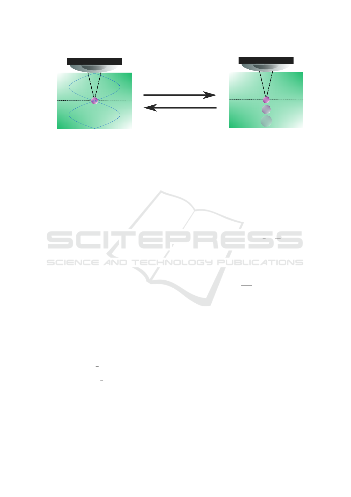
Figure 2: The hardware follows the same setup used by (Massa et al., 2023). Figure above illustrates the main stages of the

process. (a) When the actuator is on, a generated acoustic standing wave traps the particle in the microscope confocal plane.

(b) When the actuator is turned off, as the acoustic wave vanishes, the particle falls to the bottom of the cavity (perpendicular

to the confocal plane) and presents the physical behaviour explained in Section 2.1.

the particle. The acoustic wave frequency is carefully

deﬁned so that the levitation node plane matches the

confocal plane of the microscope. Once the actuator

is turned off, the particle starts to fall along the ﬂuid,

moving away from the microscope’s confocal plane,

as shown in Fig. 2 (b). Due to this displacement, sub-

sequent images acquired from the particle present in-

creasingly higher amounts of blur, which can be seen

as an increase in their area. Thus, a relationship be-

tween particle area, fall velocity and, consequently,

particle density can be established. During the course

of this work we attempted the usage of a computer

vision approach to measure the density of a 10µm di-

ameter polystyrene bead, which has a known density

of around 1050 kg·m

−3

. We also utilized a solution

with density of ρ

f luid

= 997 kg·m

−3

and a dynamic

viscosity of µ = 0.89 × 10

−1

Pa·s along with a gravi-

tational acceleration of g = 9.82 m·s

−2

2.1 Physical Background

The velocity with which a particle falls when embed-

ded in a ﬂuidic medium is directly related to its den-

sity. When the particle is approximated by a perfect

sphere, this relation is mainly controlled by gravita-

tional (Eq. 1), buoyancy (Eq. 2) and viscosity (Eq. 3)

forces (Zhao et al., 2014), i.e.;

πgr

particle

, (1)

= −

πgr

f luid

, (2)

and

= 6πrµv, (3)

where:

• ρ

particle

: Particle density.

• ρ

f luid

: Fluid density.

• r: Particle spherical approximation radius.

• µ: Fluid dynamic viscosity.

• g: Gravitational acceleration.

• v: Particle velocity.

The resulting force pulls the particle down to the

bottom of the cavity in which it is inserted and can be

found by the application of Newton’s Second Law.

∑

F = F

+ F

πr

(4)

Solving the ﬁrst order differential Eq. 4 and subse-

quently simplifying the results, it is possible to reach

the equation that describes the physical relation be-

tween fall velocity and particle density:

particle

9µv

+ ρ

f luid

. (5)

2.2 Dataset

As previously stated, we apply an optical micro-

scope to extract images from particle fall experiments.

The original images obtained by the microscope are

monochromatic (grayscale) and have a resolution of

2448×1920 pixels. Used images are 500×500 pixels

containing a single particle during the settlement pro-

cess. This resolution allows us to capture the whole

particle across the entire size range observed in exper-

iments due to the defocus.

Conducting the discussed experiments typically

presents signiﬁcant challenges. It is very common for

particles to group together in packs. In this way, the

number of images that enable the analysis of isolated

particles is extremely reduced, leading to a challeng-

ing problem. Only two successful experiments could

deliver calibration and test image sets. The calibration

set was comprised of 18 images acquired during the

VISAPP 2024 - 19th International Conference on Computer Vision Theory and Applications

438

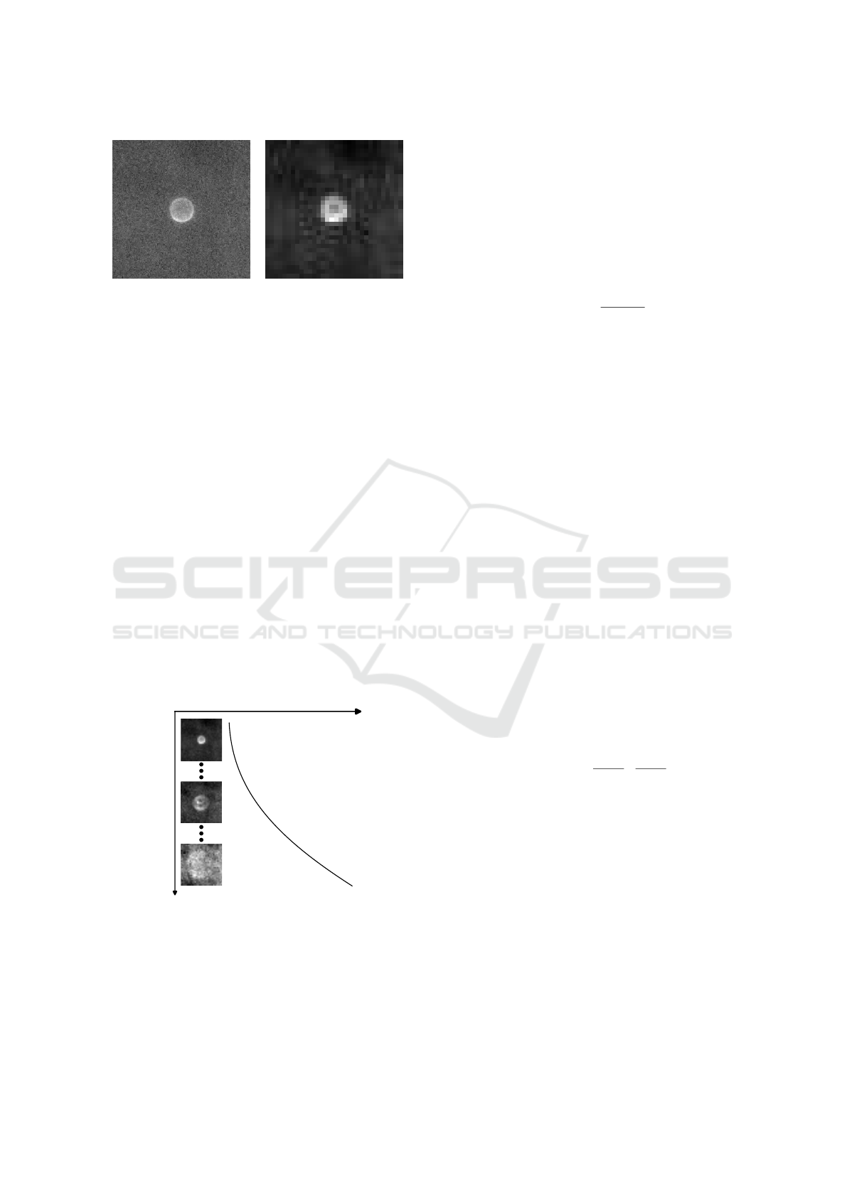
(a) Original image. (b) Preprocessed image.

Figure 3: Example of the images obtained through the ex-

plained pipeline. The left one represents the original image.

The right one represents the result after preprocessing.

particle settlement. The test set consisted of 13 im-

ages acquired in the same manner. With such limited

number of examples, the risk of overﬁtting was man-

aged with the adjustment of model’s hyperparameters

to reduce its complexity (cf. Sec. 2.5).

For the sake of reproducibility, we applied the

same preprocessing steps used in (Massa et al., 2023)

to each acquired image. The preprocessing stage in

our approach involves cropping, resizing, and enhanc-

ing, as illustrated in Fig. 1. Examples can be observed

in Fig. 3. It is also worth noting that last images in the

sequence, where the particle is close to cavity’s bot-

tom, are very noisy and unfocused, making it hard

to segment the particle via classical image process-

ing approaches. This noisy behaviour can be seen in

the bottom particle image from Fig. 4 and also in the

input image from Fig. 5.

2.3 Calibration

Relative Area

Height

Calibration curve

Figure 4: Illustration of the calibration process. As the par-

ticle falls, the blur causes an increase in the area related to

the particle’s height in each image. This relationship can be

expressed as a calibration curve.

When the particle falls, the distance to the image con-

focal plane becomes larger, resulting in a defocus that

“increases” the particle size in the acquired images.

Therefore, the dynamics of a particle embedded into

a ﬂuidic medium can be analyzed by knowing its area

and height in each image acquired during the fall pro-

cess. To do so, we ﬁt a calibration curve capable

of modeling the correspondence between the relative

area of the particle in each image and the respective

height relative to the bottom of the chamber.

For a set of n acquired images, relative area values

can be calculated with the following equation:

i relative

− A

(6)

where A

, A

, and A

are, respectively, area values for

the ﬁrst, current, and last captured images.

The computed values for relative area and their re-

spective height values can ﬁt an exponential function,

as illustrated in Fig. 4, which is used as a calibra-

tion curve. With this curve, it is possible to obtain

the height of a different particle by giving as input

the area value, as long as the studied particle has the

same diameter as the calibrated one. Finally, the fall

velocity can be derived from the height values and

used along with Eq.(5) to calculate the particle den-

sity. This highlights the importance of obtaining an

efﬁcient and automated way to estimate the particle

area, a process which, in general, is done manually.

2.4 Baseline

To serve as a baseline for further investigations, we

applied the Gaussian curve ﬁtting approach proposed

by (Massa et al., 2023) to the task of estimating parti-

cle areas. The main idea is to ﬁt a Gaussian model to

the image by minimizing an error function. As we are

dealing with images, we need to use the 2D version

of the Gaussian curve, which can be generated by the

following expression:

G(x, y) = α e

−



(x−µ

)

2σ

(y−µ

)

2σ



(7)

where:

• α: Gaussian amplitude.

• µ

: Position of the Gaussian’s center in the image

along the horizontal axis.

• µ

: Position of the Gaussian’s center in the image

along the vertical axis.

• σ: Standard deviation of the Gaussian.

As discussed in (Massa et al., 2023), deﬁning val-

ues for α, µ

, µ

and σ

which generate a Gaussian

that ﬁts a speciﬁc image is not trivial. Furthermore, as

the particle is centered in the image, µ

and µ

were

always zero, and we only had to optimize α and σ.

Thus, aiming to reproduce the experiment, we also

Assessing the Performance of Autoencoders for Particle Density Estimation in Acoustoﬂuidic Medium: A Visual Analysis Approach

439

delegated this task to a Genetic Algorithm approach.

The evolutionist theory inspires this algorithm and is a

common choice for optimization tasks (Katoch et al.,

2021).

One core concept of this method is ﬁtness, which

is the metric that determines how much an individ-

ual is adapted to the problem it intends to solve. This

metric is deﬁned according to the problem necessi-

ties. As we need to measure the error between a 2D

Gaussian-generated image and the particle image, the

Mean Squared Error was chosen as the ﬁtness metric.

Considering the particle image I(x, y) and the Gaus-

sian G(x, y), where x and y are the pixel coordinates,

the Mean Squared Error can be calculated by the fol-

lowing expression:

MSE =

W H

∑

x=1

∑

y=1

[I(x, y) − G(x, y)]

(8)

where W and H are, respectively, the width and height

of the images.

First, we used the calibration image set, which had

previously known area and height values, to calculate

a calibration curve, as discussed in Section 2.3. Then,

the test set was applied to the Genetic Algorithm op-

timization, which was executed for 1000 generations

with a population of 100 individuals. We also applied

an elitist selection by, in each generation, maintaining

the most adapted half of the population and mixing

it with the newly generated individuals. The calcu-

lated Gaussian curves were used to estimate the par-

ticle area in each image, which served as input to the

calibration curve to reach height values for the test

images and, subsequently, particle fall velocity and

density.

2.5 Autoencoder

As stated in Section 1, autoencoders (AEs) are a pow-

erful type of neural network. Their architecture com-

prises two main parts: an encoder and a decoder. The

encoder is formed by a set of layers that consecutively

reduces the dimensionality of data until it reaches the

intermediary layer, also known as bottleneck. On the

other hand, the decoder aims to reconstruct the in-

put data from the values delivered by the intermediary

layer. Both encoder and decoder can be composed of

various combinations of layer types, including convo-

lutional layers, which are ideal for computer vision-

related tasks.

The main goal of autoencoders is to reduce dimen-

sionality so the input data is compressed into mean-

ingful representations. This is done by minimizing

the distance between an input and its respective re-

construction. Encoded data is projected into a so-

ENCODER

LATENT SPACE

Convolutional: 16 kernels (3x3) - ReLU

DECODER

Dense: 1 unit - Linear

Dense: 256 units - Sigmoid

Convolutional: 16 kernels (3x3) - ReLU

Dense: 512 units - Sigmoid

Deconvolutional: 8 kernels (3x3) - ReLU

PROPORTIONAL

TO PARTICLE

AREA

NETWORK

INPUT

NETWORK

OUTPUT

LATENT

VALUE

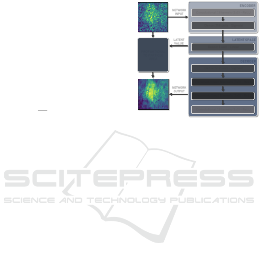
Figure 5: Autoencoder architecture diagram. Images on the

left side show examples of a particle image (upper) given as

input and a reconstructed image (lower) received as output.

The latent space is represented by a single dense unit and

is expected to contain relevant information about the parti-

cle contained in the input image, more speciﬁcally about its

area.

called latent representation space. This approach also

forces the model to focus on features with high vari-

ability, being well-suited to denoising tasks (Pratella

et al., 2021). As exposed by (Bank et al., 2020), an

AE can be formally deﬁned as learning the functions

F : R

→ R

and G : R

→ R

that satisfy the expres-

sion

argmin

F,G

E[L (x, G ◦ F(X))], (9)

where L is the reconstruction loss function and E is

the expectation over the distribution of the input x.

Furthermore, F, G, n, and l represent the encoder, the

decoder, the input data dimension and the latent space

dimension, respectively.

In this phase of our methodology, we intended to

test the limits of this architecture by squeezing parti-

cle images into a latent vector comprised by a single

real value. The purpose was to validate if the network

could extract a value proportional to the particle area

in each image through the encoder.

To do so, we used the same calibration and test im-

ages, which is a challenge due to the small number of

examples. The AE followed a simple and asymmetric

architecture, as seen in Fig. 5. The encoder was com-

prised of a single convolutional layer followed by a

dense layer that was later squeezed into a single neu-

ron. The decoder, in turn, was formed by a dense layer

followed by two deconvolutional layers.

First, we trained the autoencoder using the cali-

bration set. The target was to reconstruct the original

VISAPP 2024 - 19th International Conference on Computer Vision Theory and Applications

440

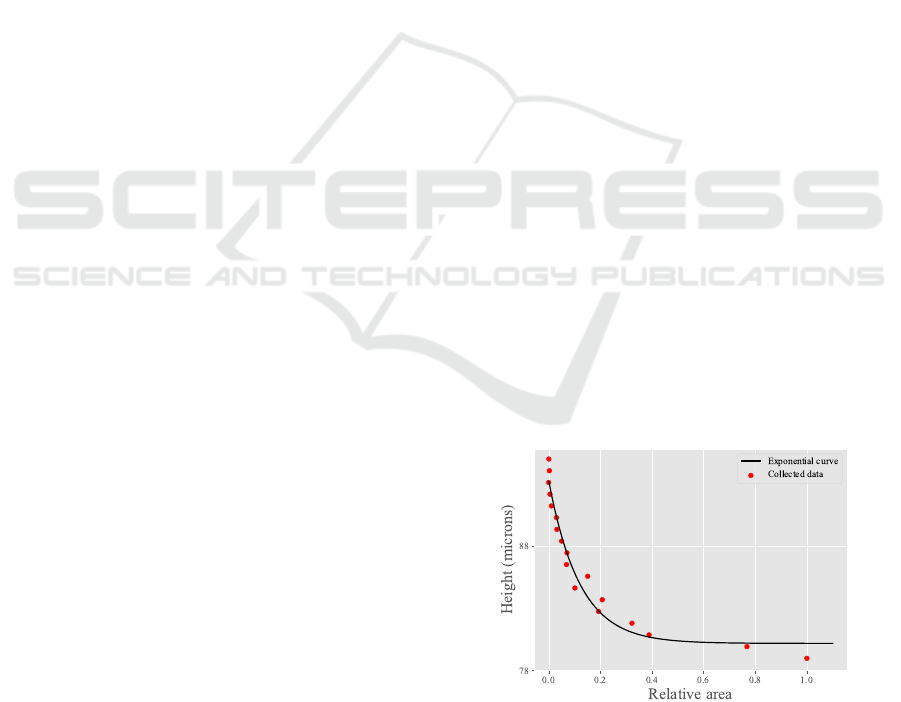
image after squeezing it to a single value. The train-

ing loop was executed for 1000 epochs. Was used the

Adam optimizer along with a learning rate of 10

−3

and a batch size of 1. As we are dealing with images,

the MSE was chosen as the loss function. No area tar-

gets were given to the latent space layer. This step is

represented by the training section in Fig. 1.

After the training, we extracted the values deliv-

ered by the latent space for each calibration image and

ﬁt them to an exponential curve. As we are dealing

with relative areas, values used to generate the cali-

bration curve do not need to be the exact areas of each

particle, as long as they are proportional to them.

Lastly, as shown in the inference section of Fig.

1, the test set was also given as input to the trained

network to obtain latent space values expected to be

proportional to the particle area. These values were

later used as input to the calibration curve to estimate

particle height. As in Section 2.4, the resulting height

values for the test images were used to derive the fall

velocity and, consequently, estimate the particle den-

sity.

All experiments were performed on a computer

with the following settings: an Intel Core i7-9700

CPU, 32GB RAM, and RTX 2060 GPU. For a fair

comparison with the baseline work, the GPU is only

used during training, leaving the CPU exclusively for

inference time calculation. Also, we used Python

3 language along with TensorFlow 2.8 (Keras) and

OpenCV 4.7 for training and inference.

3 RESULTS AND DISCUSSION

3.1 Baseline Results

After applying the pipeline proposed in Section 2.4,

we could estimate the area of the test images. The

particle radius was manually extracted for each cali-

bration image and converted via a pixel-nanometer re-

lation. By considering the particles as a perfect circle,

we calculated their areas. These values were used,

along with previously known height, to generate the

calibration curve, as discussed in section 2.3.

Compared to the results obtained by (Massa et al.,

2023), the genetic algorithm showed some lack of

performance. Despite ﬁnding good parameters for

the 2D Gaussian functions on most test images, the

curve sometimes did not ﬁt the particle correctly. The

obtained Gaussian curves were then used to compute

particle areas in each image and generate relative area

values by applying Eq. (6). Such values served as in-

put for the calibration curve. By deriving the fall ve-

locity and applying the result to Eq. (5), we could cal-

culate the particle density. The lack of performance

from the Genetic Algorithm was translated in a den-

sity estimation of 999 kg·m

−3

, which is farther from

the real value when compared to the 1059 kg·m

−3

ob-

tained by (Massa et al., 2023).

Even though the resulting density was reasonable,

the baseline approach presented some other limita-

tions. The main problem, as discussed in Section

1, is the lack of replicability, as the Genetic Algo-

rithm must be executed for each new image that will

be applied to the pipeline. Furthermore, the neces-

sity of rerunning the algorithm leads to a time efﬁ-

ciency problem, as the optimization loop takes, on

average, 13 minutes to ﬁnish (Table 1). The man-

ual extraction of the particle radius for the calibration

step is also worth mentioning, which can lead to er-

rors more easily when compared to an automated and

well-designed area extraction algorithm.

3.2 Autoencoder Results

By applying the methodology proposed in Section

2.5, we could as well estimate the density of the

polystyrene bead. The values extracted from the au-

toencoder latent space showed a valid proportional-

ity concerning the expected area values, as the ob-

tained relative areas could be successfully ﬁtted to an

exponential function, which is exposed in Figure 6.

Then, we input the test image set to the autoencoder

and used the resulting values to calculate their relative

areas. As in Section 3.1, we applied the calibration

curve to extract a height curve, which can be seen in

Fig. 7. In order to determine the fall velocity we con-

sidered this curve along with the time between each

consecutively captured images, calculating the mean

value of height variations for each interval. The veloc-

ity was ﬁnally applied to estimate the particle density.

Figure 6: Calibration curve calculated by ﬁtting height and

relative area values obtained from the autoencoder to an ex-

ponential function.

Using the same experiment conﬁguration as in

Section 3.1, this approach achieved a result of

Assessing the Performance of Autoencoders for Particle Density Estimation in Acoustoﬂuidic Medium: A Visual Analysis Approach

441

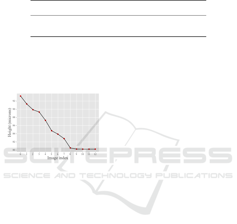
Table 1: Model Performance.

Model

Predicted

density

Absolute

error

Mean

inference time

Previous work (Massa et al., 2023) 1059 kg·m

−3

0.8% -

Baseline experiment 999 kg·m

−3

4.85% 13 minutes

Autoencoder (Ours) 1005 kg·m

−3

4.28% 6.4ms

This table summarizes the experiments discussed in this paper. The best results from the conducted ex-

periments are highlighted in bold.

1005 kg·m

−3

, which represents an absolute error of

4.28% ( Table 1). This represents some reasonable

performance, specially considering the small number

of training images. Compared to the baseline exper-

iment, this method could achieve a better result and

was executed without manual information extraction.

Figure 7: Height curve obtained by giving the relative areas

calculated through the autoencoder for the test set as input

to the calibration curve.

Moreover, after training, the AE can be applied to

any new image, without retraining. This is important

due to the fact that the baseline approach is done by

a classical Genetic Algorithm, which runs an iterative

optimization process. This process does not create a

model capable of generalizing for new inputs. Thus,

there is an increase in the computational cost of the

pipeline, as the optimization process needs to be run

for each new input image.

Lastly, the neural network is more time efﬁcient

and can be trained faster than the Genetic Algorithm.

Indeed, the AE took approximately 2.5 minutes to

train along 1000 epochs in the hardware described

in Section 2.5. Moreover, regarding the Genetic Al-

gorithm (GA) optimization loop time as its inference

time, the AE is also much more efﬁcient, presenting

a mean prediction time of only 6.4ms for each input

image, without using a GPU. The GA, on the other

hand, delivered a much higher prediction time of 13

minutes. Results are summarized in Table 1.

It is also worth mentioning that the resulting curve

obtained with the autoencoder (Fig. 7) exposes satura-

tion of some height values. This can be seen in the last

4 points since, despite the fact that the particle was

still falling, the network predicted similar area values,

resulting in an almost constant curve. We believe that

some limitations of the AE might cause this in dealing

with data outside of its training range (original man-

ifold). In this way, if an image with a larger particle

than the ones presented during the training is given

as input, the value returned by the latent space might

be saturated and lead to wrong predictions. Thus, we

intend to investigate this scenario in future work.

4 CONCLUSIONS

In this paper, we reproduced a previous work and pro-

posed a method to estimate the density of particles on

a microscopic scale using acoustoﬂuidics and com-

puter vision. Aiming at obtaining an automated par-

ticle area extraction, we proposed the use of a simple

convolutional autoencoder (AE) architecture capable

of reconstructing the input image while delivering,

through its latent space layer, a value proportional to

the particle area. The model was trained with a cali-

bration set and the values returned by the latent space

were used to ﬁt a calibration curve. Then, test im-

ages were given as input to the autoencoder and the

resulting latent values were used along with the cali-

bration curve to estimate the fall velocity and, ﬁnally,

the particle density.

Our experiments revealed a reasonable perfor-

mance for the AE model, estimating a density of

1005 kg·m

−3

which improves the baseline approach.

The network also vastly outperforms the baseline

model when considering the efﬁciency and usability,

as it has a much quicker inference time and does not

require retraining for a new experiment.

As future work, we intend to analyze the applica-

bility of VAEs, as they tend to learn continuous latent

spaces that allow the generation of data from values

outside the training range, a property that can help

in mitigating the saturation that was previously dis-

cussed. It is also worth investigating an increase in

the amount of bottleneck neuron units, as it may be

VISAPP 2024 - 19th International Conference on Computer Vision Theory and Applications

442

capable of learning a latent space that, besides parti-

cle area, can describe other important image features.

ACKNOWLEDGEMENTS

This project was supported by the Science, Tech-

nology and Innovations Ministry of Brazil, with re-

sources from law nº 8.2428 of October 23, 1991

within the Softex

National Innovation Priority pro-

gram, coordinated by Softex and EDGE Innovation

Center and published by [RESIDENCIA EM TIC ˆ

09(process[01245.005714/2022-18])].

REFERENCES

Bank, D., Koenigstein, N., and Giryes, R. (2020). Autoen-

coders. arXiv preprint arXiv:2003.05991.

Bryan, A. K., Goranov, A., Amon, A., and Manalis, S. R.

(2010). Measurement of mass, density, and volume

during the cell cycle of yeast. Proceedings of the Na-

tional Academy of Sciences, 107(3):999–1004.

Castiglioni, M., Rivoira, L., Ingrando, I., Del Bubba, M.,

and Bruzzoniti, M. C. (2021). Characterization tech-

niques as supporting tools for the interpretation of

biochar adsorption efﬁciency in water treatment: A

critical review. Molecules, 26(16).

De Pastina, A., Maillard, D., and Villanueva, L. (2018).

Fabrication of suspended microchannel resonators

with integrated piezoelectric transduction. Microelec-

tronic Engineering, 192:83–87.

Ignatans, R., Ziatdinov, M., Vasudevan, R., Valleti, M.,

Tileli, V., and Kalinin, S. V. (2022). Latent mecha-

nisms of polarization switching from in situ electron

microscopy observations. Advanced Functional Ma-

terials, 32(23):2100271.

Kalinin, S. V., Dyck, O., Jesse, S., and Ziatdinov, M.

(2021a). Exploring order parameters and dynamic

processes in disordered systems via variational au-

toencoders. Science Advances, 7(17):eabd5084.

Kalinin, S. V., Zhang, S., Valleti, M., Pyles, H., Baker, D.,

De Yoreo, J. J., and Ziatdinov, M. (2021b). Disentan-

gling rotational dynamics and ordering transitions in

a system of self-organizing protein nanorods via ro-

tationally invariant latent representations. ACS nano,

15(4):6471–6480.

Katoch, S., Chauhan, S. S., and Kumar, V. (2021). A re-

view on genetic algorithm: past, present, and future.

Multimedia Tools and Applications, 80:8091–8126.

Li, P. and Huang, T. J. (2018). Applications of acoustoﬂu-

idics in bioanalytical chemistry. Analytical chemistry,

91(1):757–767.

Maric, D., Maric, I., and Barker, J. L. (1998). Buoyant den-

sity gradient fractionation and ﬂow cytometric analy-

https://softex.br/

sis of embryonic rat cortical neurons and progenitor

cells. Methods, 16(3):247–259.

Massa, L., Vieira, T. F., de Medeiros Martins, A., Ara

ujo,

I. B. Q., Silva, G. T., and Santos, H. D. A. (2023).

Model ﬁtting on noisy images from an acoustoﬂu-

idic micro-cavity for particle density measurement. In

VISIGRAPP.

Minelli, C., Sikora, A., Garcia-Diez, R., Sparnacci, K.,

Gollwitzer, C., Krumrey, M., and Shard, A. G. (2018).

Measuring the size and density of nanoparticles by

centrifugal sedimentation and ﬂotation. Analytical

Methods, 10(15):1725–1732.

uisch, C. S., Stuckert, R., and Wittemann, A. (2021). Di-

rect measurement of sedimentation coefﬁcient distri-

butions in multimodal nanoparticle mixtures. Nano-

materials, 11(4).

Pratella, D., Ait-El-Mkadem Saadi, S., Bannwarth, S.,

Paquis-Fluckinger, V., and Bottini, S. (2021). A sur-

vey of autoencoder algorithms to pave the diagnosis

of rare diseases. International journal of molecular

sciences, 22(19):10891.

Rasouli, R., Villegas, K. M., and Tabrizian, M. (2023).

Acoustoﬂuidics–changing paradigm in tissue engi-

neering, therapeutics development, and biosensing.

Lab on a Chip, 23(5):1300–1338.

Ullmann, C., Babick, F., Koeber, R., and Stintz, M. (2017).

Performance of analytical centrifugation for the parti-

cle size analysis of real-world materials. Powder Tech-

nology, 319:261–270.

Uttinger, M. J., Boldt, S., Wawra, S. E., Freiwald, T. D.,

Damm, C., Walter, J., Lerche, D., and Peukert, W.

(2020). New prospects for particle characteriza-

tion using analytical centrifugation with sector-shaped

centerpieces. Particle & Particle Systems Characteri-

zation, 37(7):2000108.

Wu, M., Ozcelik, A., Rufo, J., Wang, Z., Fang, R., and

Jun Huang, T. (2019). Acoustoﬂuidic separation of

cells and particles. Microsystems & nanoengineering,

5(1):32.

Xie, Y., Bachman, H., and Huang, T. J. (2019). Acoustoﬂu-

idic methods in cell analysis. TrAC Trends in Analyti-

cal Chemistry, 117:280–290.

Yazdani, A. M. and S¸ is¸man, A. (2020). A novel numeri-

cal model to simulate acoustoﬂuidic particle manipu-

lation. Physica Scripta, 95(9):095002.

Zhao, Y., Lai, H. S. S., Zhang, G., Lee, G.-B., and Li, W. J.

(2014). Rapid determination of cell mass and density

using digitally controlled electric ﬁeld in a microﬂu-

idic chip. Lab on a Chip, 14(22):4426–4434.

Assessing the Performance of Autoencoders for Particle Density Estimation in Acoustoﬂuidic Medium: A Visual Analysis Approach

443