Challenging the Black Box: A Comprehensive Evaluation of Attribution

Maps of CNN Applications in Agriculture and Forestry

Lars Nieradzik

1 a

, Henrike Stephani

1 b

, J

ordis Sieburg-Rockel

3 c

, Stephanie Helmling

3 d

Andrea Olbrich

3 e

and Janis Keuper

2 f

Image Processing Department, Fraunhofer ITWM, Fraunhofer Platz 1, 67663, Kaiserslautern, Germany

Institute for Machine Learning and Analysis (IMLA), Offenburg University, Badstr. 24, 77652, Offenburg, Germany

unen Institute of Wood Research, Leuschnerstraße 91, 21031, Hamburg, Germany

Keywords:

Explainable AI, Class Activation Maps, Saliency Maps, Attribution Maps, Evaluation.

Abstract:

In this study, we explore the explainability of neural networks in agriculture and forestry, speciﬁcally in fer-

tilizer treatment classiﬁcation and wood identiﬁcation. The opaque nature of these models, often considered

’black boxes’, is addressed through an extensive evaluation of state-of-the-art Attribution Maps (AMs), also

known as class activation maps (CAMs) or saliency maps. Our comprehensive qualitative and quantitative

analysis of these AMs uncovers critical practical limitations. Findings reveal that AMs frequently fail to

consistently highlight crucial features and often misalign with the features considered important by domain

experts. These discrepancies raise substantial questions about the utility of AMs in understanding the decision-

making process of neural networks. Our study provides critical insights into the trustworthiness and practi-

cality of AMs within the agriculture and forestry sectors, thus facilitating a better understanding of neural

networks in these application areas.

1 INTRODUCTION

The application of neural networks in agriculture and

forestry has proven beneﬁcial in various tasks such

as wood identiﬁcation (Nieradzik et al., 2023), plant

phenotyping, yield prediction, and disease detection.

However, a signiﬁcant roadblock to wider adoption is

the inherently opaque nature of these models, which

tends to dampen user conﬁdence due to their limited

explainability.

Wood identiﬁcation serves as a prime example of

this challenge. It remains unclear whether the de-

cisions of neural networks focus on the same set of

features as a human expert would. Humans use 163

structural features deﬁned by the International Asso-

ciation of Wood Anatomists (Wheeler et al., 1989) for

microscopic descriptions of approximately 8,700 tim-

https://orcid.org/0000-0002-7523-5694

https://orcid.org/0000-0002-9821-1636

https://orcid.org/0009-0001-7547-269X

https://orcid.org/0009-0009-6611-3140

https://orcid.org/0009-0007-2249-2797

https://orcid.org/0000-0002-1327-1243

bers, as collected in various databases (Richter and

Dallwitz, ards; Wheeler, ards; Koch and Koch, 2022).

To demystify these black-box models, Attribution

Methods have emerged as standard tools for visualiz-

ing the decision processes in neural networks (Zhang

et al., 2021b). These methods, particularly relevant

in Computer Vision tasks with image inputs, com-

pute Attribution Maps (AMs), also known as Saliency

Maps, for individual images based on trained mod-

els. AMs aim to provide human-interpretable visu-

alizations that reveal the weighted impact of image

regions on model predictions, enabling intuitive ex-

planations of the complex internal mappings. Despite

their potential, the practical adoption of AMs in vari-

ous domains remains limited.

Addressing this gap, our paper conducts a thor-

ough evaluation of multiple state-of-the-art attribution

maps using two real-world datasets from the agricul-

ture and forestry domain. We have trained state-of-

the-art Convolutional Neural Networks (CNNs) on a

wood identiﬁcation dataset and a dataset concerning

fertilizer treatments for nutrient deﬁciencies in winter

wheat and winter rye. The key contributions of this

paper include:

Nieradzik, L., Stephani, H., Sieburg-Rockel, J., Helmling, S., Olbrich, A. and Keuper, J.

Challenging the Black Box: A Comprehensive Evaluation of Attribution Maps of CNN Applications in Agriculture and Forestry.

DOI: 10.5220/0012363400003660

Paper published under CC license (CC BY-NC-ND 4.0)

In Proceedings of the 19th International Joint Conference on Computer Vision, Imaging and Computer Graphics Theory and Applications (VISIGRAPP 2024) - Volume 2: VISAPP, pages

483-492

ISBN: 978-989-758-679-8; ISSN: 2184-4321

483

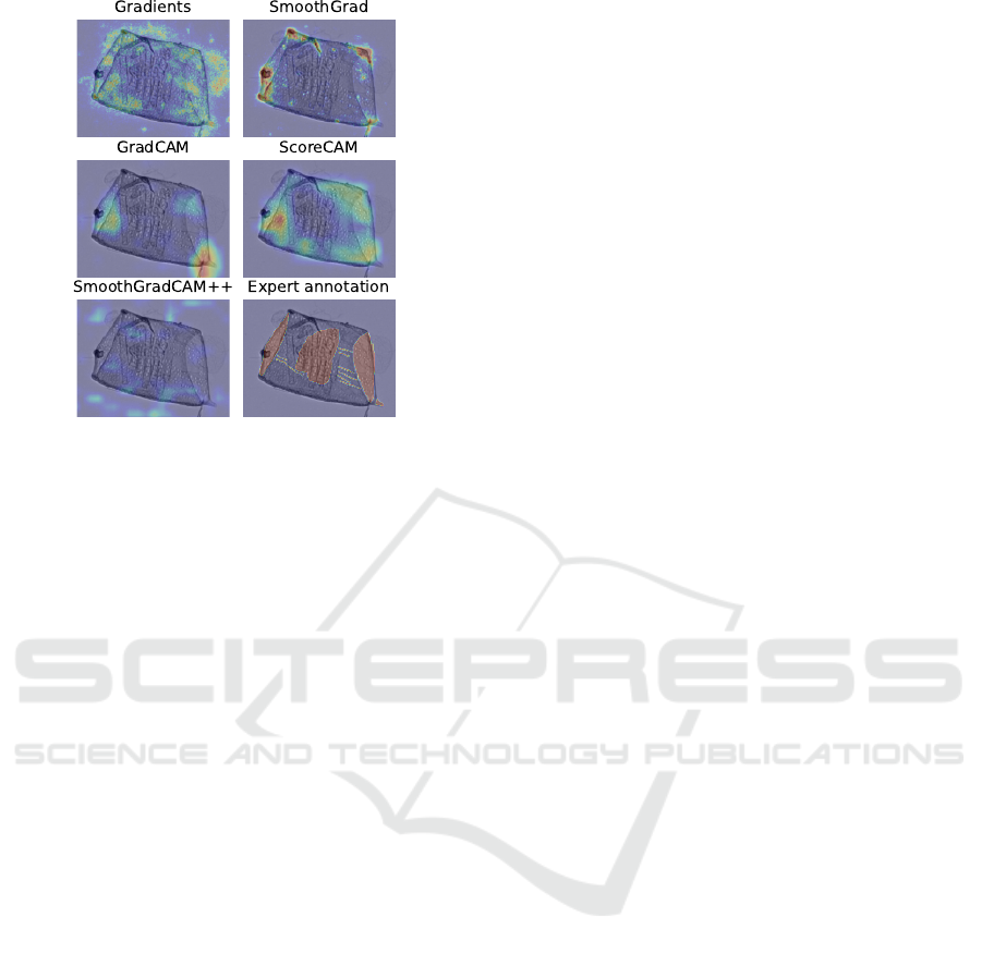
Figure 1: Visualization of different attribution maps (AM)

on the same input image of a wood identiﬁcation dataset.

All the AMs focus on different regions that are also different

from the expert annotation. Notably, SmoothGradCAM++

(Omeiza et al., 2019) appears to exclusively show noise.

• A comprehensive analysis of state-of-the-art attri-

bution maps for wood identiﬁcation and fertilizer

treatment, both qualitatively and quantitatively.

• We identify signiﬁcant variance among attribution

methods, leading to inconsistent region highlight-

ing and excessive noise in certain methods.

• Our results raise concerns regarding attribution

maps that display excessive feature sharing across

distinct classes, suggesting potential issues.

• In collaboration with wood anatomists, key fea-

tures were annotated in the wood identiﬁcation

dataset. These annotations were used to measure

the alignment with respect to the attribution maps.

Notably, none of the maps showed high alignment

with expert annotations.

By investigating these aspects, this study provides

valuable insights into the effectiveness and reliabil-

ity of attribution maps for wood species identiﬁcation

and fertilizer treatment classiﬁcation, beneﬁting do-

main experts in agriculture and forestry.

2 RELATED WORK

2.1 Attribution Methods

The ﬁeld of attribution methods has witnessed sig-

niﬁcant growth in recent years, with numerous tech-

niques being developed and widely used in the con-

text of neural networks. Full back-propagation meth-

ods, such as Gradients (Simonyan et al., 2014), have

played a fundamental role in the early approaches

to attribution maps for classiﬁcation models. These

methods compute gradients of a learned neural net-

work with respect to a given input, providing insights

into the importance of different image regions. De-

ConvNet (Zeiler and Fergus, 2013) and Guided back-

propagation (Springenberg et al., 2015) were intro-

duced as extensions to Gradients, modifying the gra-

dients to allow the backward ﬂow of negative gradi-

ents. Another variant, SmoothGrad (Smilkov et al.,

2017), enhances the gradient computation by adding

Gaussian noise to the input and averaging the results.

Path backpropagation methods take a different ap-

proach by parameterizing a path from a baseline im-

age to the input image and computing derivatives

along this path. Integrated Gradients (Sundararajan

et al., 2017), for example, uses a straight line path be-

tween a black (all-zero) image and the test input, and

integrates the partial derivatives of the neural network

along this path. Variations of Integrated Gradients,

such as Blur Integrated Gradients (Xu et al., 2020)

and Guided Integrated Gradients (Kapishnikov et al.,

2021), have been proposed to improve the path initial-

ization and computation.

Class Activation Maps (CAMs) offer an alterna-

tive to computing gradients with respect to the input.

CAM methods stop the back-propagation of gradients

at a chosen layer of the network. GradCAM (Sel-

varaju et al., 2019), a popular CAM approach, com-

putes an attribution map by summing weighted acti-

vations at the chosen layer. GradCAM++ (Chattopad-

hay et al., 2018) further enhances the original Grad-

CAM by incorporating different gradient weighting

schemes. Smooth GradCAM++(Omeiza et al., 2019)

adds Gaussian noise to the input, similar to Smooth-

Grad, to improve the visualization. Other CAM vari-

ants, such as LayerCAM (Jiang et al., 2021) and

XGradCAM (Fu et al., 2020), introduce different

weighting schemes for the computed gradients.

In contrast to gradient-based methods, ScoreCAM

(Wang et al., 2020b) does not rely on gradient compu-

tations for attribution. Instead, it measures the impor-

tance of channels in an intermediate layer by observ-

ing the change in conﬁdence when removing parts of

the activation values.

Beyond these well-known approaches, numer-

ous other attribution map methods have been pro-

posed, building upon and combining existing tech-

niques (Ancona et al., 2017). These methods in-

clude SS-CAM (Wang et al., 2020a), IS-CAM (Naidu

et al., 2020), Ablation-CAM (Desai and Ramaswamy,

2020), FD-CAM (Li et al., 2022), Group-CAM

(Zhang et al., 2021a), Poly-CAM (Englebert et al.,

VISAPP 2024 - 19th International Conference on Computer Vision Theory and Applications

484

2022), Zoom-CAM (Shi et al., 2020), and Eigen-

CAM (Muhammad and Yeasin, 2020), each introduc-

ing unique modiﬁcations and improvements to the at-

tribution map generation process.

Additionally, black-box methods offer an alterna-

tive approach by masking the input in various ways.

For instance, RISE (Petsiuk et al., 2018a) and its pre-

cursor, introduced in earlier works (Zeiler and Fergus,

2013), randomly occlude the input image and record

the resulting change in class probabilities. Several

other black-box methods have also been proposed in

the literature (Fong et al., 2019; Fong and Vedaldi,

2017; Petsiuk et al., 2018b; Ribeiro et al., 2016).

Overall, the ﬁeld of attribution methods offers

a diverse range of techniques, each with its own

strengths and limitations.

2.2 Evaluation of Attribution Methods

In this work, we aim to evaluate and compare various

state-of-the-art attribution map methods in the context

of wood species identiﬁcation and fertilizer treatment

classiﬁcation, speciﬁcally focusing on their applica-

bility and usefulness in real-world domains such as

agriculture and forestry.

A similar study conducted by (Saporta et al.,

2022) in the medical ﬁeld evaluated attribution maps

for interpreting chest x-rays. However, their analysis

focused mainly on comparing attribution maps with

human annotations. In contrast, we extend our study

to scenarios where annotations are not available. It is

important to note that annotations are not necessarily

the basis for the network’s decision. As a surrogate,

we measure the consistency between different attribu-

tion maps, use established metrics from the existing

literature, and perform a thorough qualitative analy-

sis.

In another relevant research endeavor in the area

of plant phenotyping (Toda and Okura, 2019), various

methods for visualizing network behavior were con-

sidered. While qualitative analysis is certainly valu-

able, our approach places a greater emphasis on the

quantitative aspects.

Finally, we argue for the use of modern CNN

architectures. The aforementioned works relied on

models such as InceptionV3 (Szegedy et al., 2015),

DenseNet121 (Huang et al., 2018), or ResNet152 (He

et al., 2015), which are considered somewhat out-

dated in light of the rapidly evolving ﬁeld of Deep

Learning. These models produce suboptimal results

on both standard and real-world datasets (Fang et al.,

2023). We propose to use more modern architectures

that potentially produce better class activation maps

(Liu et al., 2022) (as seen in (Tan and Le, 2019)).

3 METHOD

3.1 Consistency

The output of attribution methods are matrices, nor-

malized within the range of [0, 1]

n×m

, where n and m

represent the image’s dimensions. Given that these

matrices do not typically exhibit high structural com-

plexity necessitating adjustments for shifts or color

adaptations, we opt for straightforward metrics per-

forming pixel-wise comparisons between the saliency

maps. A low similarity index among saliency maps

indicates reduced consistency, as different regions are

deemed important by different maps. Moreover, when

all the saliency maps roughly agree with each other, it

means that the choice of the saliency map is not that

important. However, in situations where all saliency

maps disagree, one may prove superior to the rest.

We introduce two metrics to measure consistency.

The ﬁrst metric is the Pearson correlation coefﬁcient,

deﬁned as:

∑

i=1

− ¯x)(y

− ¯y)

∑

i=1

− ¯x)

∑

i=1

− ¯y)

where x

is the ith pixel in the AM and ¯x is the sam-

ple mean. Similarly, y

is the ith pixel of the second

AM. The output range of r

is [−1, 1], with 1 indicat-

ing the highest consistency and ≤ 0 a low consistency.

= 0 is intuitively random noise and r

= −1 an

”inverted” saliency map.

The second metric is the Jensen–Shannon diver-

gence (JSD). We assume that each pixel is the result of

a binary regression model, which classiﬁed the pixel

as either important or unimportant (Bernoulli distri-

bution). Then we can compare the distribution X of

this pixel against a second distribution Y to see how

similar the two distributions are.

First, let us deﬁne the Kullback–Leibler diver-

gence between all the pixels of two saliency maps.

D(X ∥ Y ) =

∑

i=1

log





+(1−x

)log



1 − x

1 − y



The formula D(X ∥ Y ), while informative, lacks

symmetry and does not have an upper bound of 1,

making the results less interpretable. To yield more

understandable numbers, we opt for JSD instead. This

is a smoothed and symmetric variant of the Kullback-

Leibler divergence, thereby offering an enhanced in-

terpretability. It is deﬁned as

0 ≤ JSD(X ∥ Y ) =

D(X ∥ M)+

D(Y ∥ M) ≤ 1 ,

where M =

(X +Y).

Challenging the Black Box: A Comprehensive Evaluation of Attribution Maps of CNN Applications in Agriculture and Forestry

485

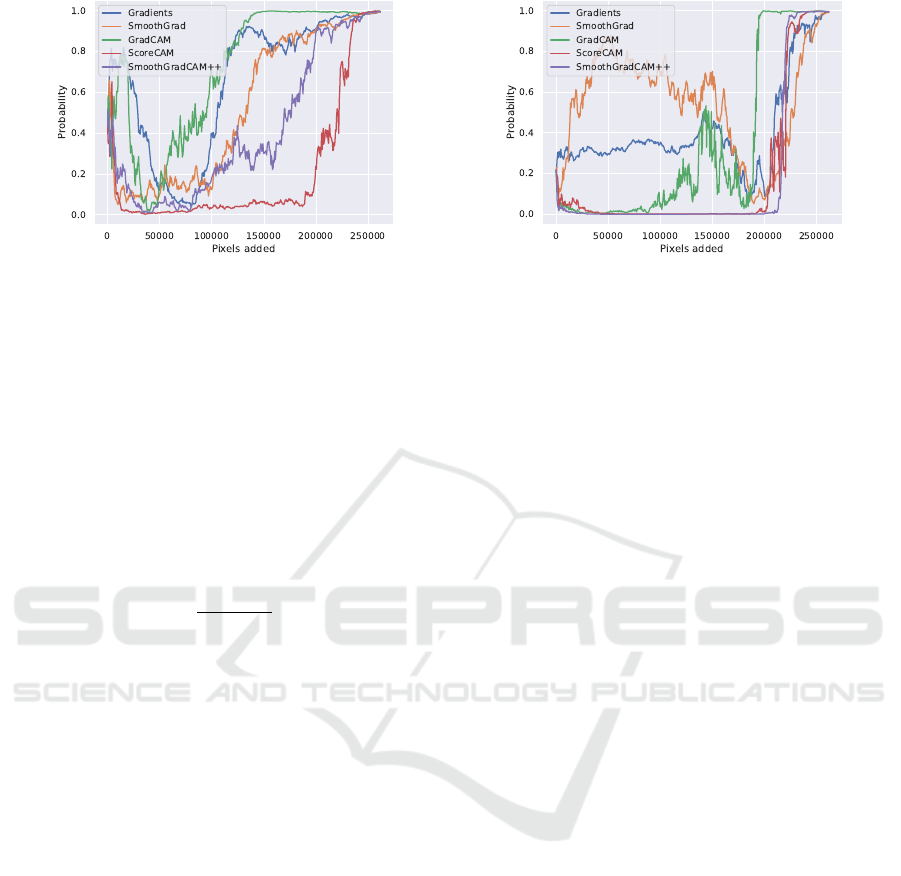
(a) Insertion with blurring. (b) Insertion without blurring.

Figure 2: The ”Insertion” metric evaluated on an example image illustrates the impact of the parameter ”blurring” in com-

parison to ”no blurring”. In (a), the starting image is a completely blurred image. In (b), the starting image is a black image.

We input this modiﬁed image into the neural network to obtain a probability (see y-axis). First, the most important pixels

of the original image are inserted. Then gradually less important pixels are inserted. At each step, the network predicts the

probability of this modiﬁed image. The process ends with the complete original image and the original probability. The best

saliency map in the plots is determined by computing the area under the curve (AUC).

The results of both metrics can be visualized in a

confusion matrix. We take the average of the upper

triangular elements of the confusion matrix to obtain

a single value. Then the consistency for Pearson’s r is

deﬁned as

Consistency

Corr

m(m − 1)

m−1

∑

i=1

∑

j=i+1

We deﬁne Consistency

JSD

in the same way.

3.2 Qualitative and Quantitative

Evaluation of Saliency Maps

In situations where saliency maps demonstrate sub-

stantial inconsistency among themselves, the selec-

tion of the most suitable saliency map for the speciﬁc

task becomes critical. Numerous metrics have been

proposed to assess the quality of these saliency maps

(Chattopadhay et al., 2018; Poppi et al., 2021; Fong

and Vedaldi, 2017; Petsiuk et al., 2018b; Gomez et al.,

2022; Zhang et al., 2016; Raatikainen and Rahtu,

2022), with the intent to discern which one is pre-

dicted to yield the best performance for a particular

dataset, or even across datasets.

Among the state-of-the-art metrics, two promi-

nent ones are ”Insertion” and ”Deletion”. These met-

rics will be utilized in our comparison analysis to

evaluate the saliency maps’ performance and deter-

mine their effectiveness.

Deletion and Insertion were proposed by (Fong

and Vedaldi, 2017) and (Petsiuk et al., 2018b). It is an

iterative process of pixel deletion or insertion within

the test image. The pixels are ordered by the impor-

tance given by the saliency map. For instance, the

deletion process initiates with the input test image,

and then sequentially masks the subsequent impor-

tant regions with a value of 0. Each modiﬁed image

is given to the neural network to produce a probabil-

ity. The ﬁrst image is the original image and the last

image is a black image. This process can be visual-

ized by plotting the count of inserted or deleted pixels

(x-axis) against the probability of the target class (y-

axis). To summarize this plot into a scalar value, the

area under the curve (AUC) is calculated.

While these evaluation methods are sensible, they

have certain intrinsic limitations. They are not com-

prehensive measures, as they overlook critical fac-

tors such as the noise level in the saliency map and

the map’s degree of user-informativeness. Moreover,

these methods are inﬂuenced by their respective pa-

rameters. Frequently, they work based on conceal-

ing parts of the image that the neural network deems

signiﬁcant. The process of obscuring these areas,

whether through blurring or masking, introduces an-

other parameter. The size of the blurring/masking ker-

nel or the number of pixels chosen for image modiﬁ-

cation at each iteration can have a signiﬁcant impact

on the metric’s result. An example can be seen in

ﬁg. 2. Therefore, it is not enough to look only at the

metrics to prove that a particular saliency map reﬂects

the correct decision process of a neural network.

Thus, visual comparison of the results with ex-

pert annotations remains indispensable for veriﬁ-

cation. Instead of comparing the attribution map

purely with previously mentioned metrics, we also

propose a comparison with manual feature annota-

tions. It is crucial to note that convolutional neu-

ral networks (CNNs) might select different image

features for decision-making than a human expert

VISAPP 2024 - 19th International Conference on Computer Vision Theory and Applications

486

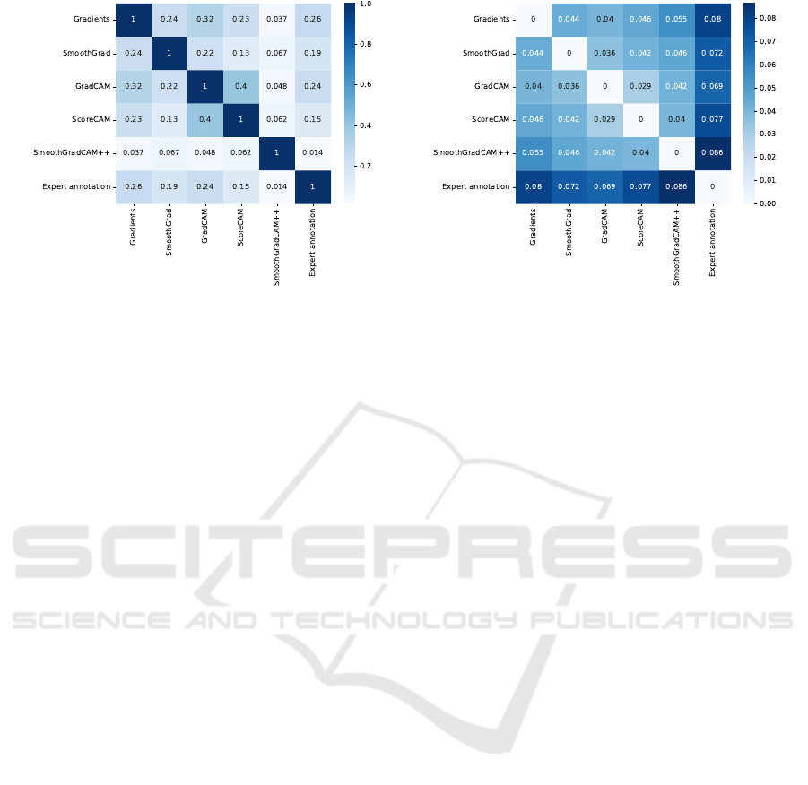
(a) Pearson correlation coefﬁcient (higher is better). (b) Jensen–Shannon divergence (lower is better).

Figure 3: This plot illustrates the degree of similarity among all attribution maps. The matrices were computed by averaging

the individual metric results across all attribution maps in the wood identiﬁcation dataset. Both similarity measures indicate a

weak agreement among the different maps.

would. Nonetheless, utilizing human annotations of-

fers a form of ”ground truth” that, while it may not

represent ”the” deﬁnitive decision-making process of

the CNN, at least provides ”a” valid process for this

classiﬁcation problem.

Finally, it is also worthwhile examining the same

saliency map of different target classes. From the

perspective of a human expert, the highlighting of a

region in the saliency map signiﬁes the presence of

a particular feature. Therefore, if a region appears

in the saliency maps of multiple classes, it suggests

that those classes share a common feature. However,

for a neural network, the decision-making process is

not solely based on the existence or absence of spe-

ciﬁc regions in the saliency map. Even a slight vari-

ation in the range of values at certain pixels can lead

to a change in the assigned class label. Therefore,

while observing features in the saliency map indi-

cates a more interpretable representation, it does not

guarantee an accurate mapping of the actual decision-

making process. The advantage of uniquely high-

lighted regions across multiple classes is that such a

saliency map method would resemble a more human-

like reasoning process.

4 EVALUATION

We perform our qualitative and quantitative analysis

on two datasets: (1) Wood identiﬁcation (Nieradzik

et al., 2023): the dataset consists of high-resolution

microscopy images for hardwood ﬁber material. Nine

distinct wood species have to be distinguished. (2)

DND-Diko-WWWR (Yi, 2023): This dataset, ob-

tained from unmanned aerial vehicle (UAV) RGB im-

agery, provides image-level labels for the classiﬁca-

tion of nutrient deﬁciencies in winter wheat and win-

ter rye. Classiﬁers are tasked with distinguishing be-

tween seven types of fertilizer treatments.

We trained CNNs for each of these datasets. The

ConvNeXt (Liu et al., 2022) architecture was selected

due to its good accuracy on real-world datasets as

demonstrated in the research by (Fang et al., 2023).

The same paper also shows that many architectures

that boast improved accuracy on ImageNet often fail

to replicate this performance on real-world datasets.

Further substantiating this choice, the study in (Nier-

adzik et al., 2023) demonstrated ConvNeXt’s supe-

rior accuracy in wood species identiﬁcation, surpass-

ing other tested architectures, and performing on par

with human experts.

In terms of the fertilizer treatment dataset, we at-

tained approximately 75% accuracy, representing a

robust baseline for our experiments. This ensures that

our models are capable at identifying key features,

critical for evaluating the attribution maps, across

both datasets. Moreover, by submitting our predic-

tions with a slightly stronger model to the fertilizer

dataset’s competition, we achieved an accuracy >

89%, further validating the effectiveness of our mod-

els.

4.1 Consistency and Expert Annotation

4.1.1 Wood Identiﬁcation Dataset

Expert wood anatomists annotated key features within

a carefully curated subset of 270 samples from this

dataset. These samples were selected for their dis-

tinct and easily discernible features. We suspect that

Challenging the Black Box: A Comprehensive Evaluation of Attribution Maps of CNN Applications in Agriculture and Forestry

487

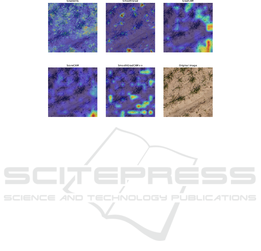
Figure 4: Visualization of different attribution maps for the fertilizer dataset of an individual image. Similar to the maps for

the wood identiﬁcation dataset, they exhibit inconsistency in identifying what they consider important.

the neural network may also base its decision on these

features. All experiments were conducted using these

270 samples. Empirical tests conﬁrmed that increases

in sample size did not affect the outcomes, thus estab-

lishing the statistical signiﬁcance of the results.

For our initial experiment, we examine the con-

sistency among various attribution maps. As demon-

strated in ﬁg. 3, there is only a marginal correla-

tion between different saliency maps. We obtained a

Consistency

Corr

of 0.17 and a Consistency

JSD

of 0.05.

Both measures similarly rank the consistency across

most methods.

Notably, only GradCAM and ScoreCAM demon-

strate a reasonably high level of agreement. This can

be attributed to the fact that both methods utilize the

pre-logit output feature matrix, whereas other meth-

ods depend on backpropagation from the output to the

input image. However, even in this case, the correla-

tion coefﬁcient shows an agreement barely over 40%.

The visual display of attribution maps for an individ-

ual vessel, as depicted in ﬁg. 1 on the front page, fur-

ther underscores this disparity.

This ﬁnding is surprising given that the task of

wood species identiﬁcation is well-deﬁned in terms

of expert consensus on important features. Hence, the

saliency maps’ behavior diverges from that of human

experts.

Upon considering the expert annotation, we ob-

serve that the Gradients method shows the highest

similarity with Pearson’s correlation coefﬁcient, al-

beit the agreement falls short of 30%. Another less

apparent issue is the high noise level associated with

this method, which complicates the interpretation of

results. Conversely, GradCAM and ScoreCAM of-

fer more comprehensible visual explanations, as they

are not inﬂuenced by backpropagation through mul-

tiple distinct layers. In terms of JSD, GradCAM is

deemed the most similar to expert annotation, which

aligns more closely with expectations from visual in-

spection.

4.1.2 Fertilizer Treatment Dataset

Similar to the Wood identiﬁcation dataset, we use

around 300 images for performing tests and comput-

ing the metrics.

Despite the fertilizer dataset comprising entirely

different images, it still exhibits similar inconsistency

patterns as witnessed in the previous dataset. With

our deﬁned metrics, we measured a Consistency

Corr

of 0.1 and a Consistency

JSD

of 0.06. The correlation

coefﬁcient is even lower for this dataset. Both con-

fusion matrices have similar values as the one for the

wood identiﬁcation dataset.

As demonstrated visually in ﬁg. 4, all the attribu-

tion maps identify varying regions as signiﬁcant. In

parallel with our earlier observations, we note a sub-

stantial amount of noise within the method Gradients.

4.2 Metrics and Feature Sharing

As seen in the previous section, attribution maps lack

consistency, underscoring the importance of selecting

the most suitable map for the task at hand.

VISAPP 2024 - 19th International Conference on Computer Vision Theory and Applications

488

(a) GradCAM. (b) SmoothGrad.

Figure 5: Attribution maps are intended to visualize the most crucial regions inﬂuencing the decision for a speciﬁc class in a

given model. However, this image comparison reveals that both saliency maps highlight vastly different regions for each class,

even though we aim to visualize the same model and classes. SmoothGrad tends to highlight the same regions regardless of

the correct class (Euca), whereas GradCAM emphasizes distinct regions. This lack of consistency raises uncertainty about

which region the model truly deems most important, making it challenging to identify easily interpretable features for humans.

4.2.1 Wood Identiﬁcation Dataset

We evaluated the maps using two metrics – ”Inser-

tion” and ”Deletion”, as seen in table 1.

Table 1: Evaluation of the attribution methods using ”Dele-

tion” and ”Insertion”. The metrics do not provide a conclu-

sive answer on which saliency map is best.

Attribution Method Deletion ↓ Insertion ↑

GradCAM 0.4622 0.9899

ScoreCAM 0.5302 0.9783

SmoothGradCAM++ 0.5885 0.9372

Gradients 0.2183 0.9099

SmoothGrad 0.2741 0.9552

Expert annotation 0.6868 0.8908

Interestingly, the metrics suggest differing ”best”

attribution methods: ”Deletion” points to Gradients

as superior, while ”Insertion” favors GradCAM. Fur-

thermore, neither metric rates the expert annotation

highly. This divergence might indicate that the neural

network is learning different features from those that

human experts would typically recognize.

However, an alternative explanation could be that

these metrics themselves may not be fully suitable

as evaluation measures. Ideally, we would employ a

”metric of a metric” that evaluates the effectiveness of

the evaluation metrics themselves. In absence of such

a measure, we ﬁnd ourselves in a situation where ”In-

sertion” and ”Deletion” suggest different ”best” attri-

bution maps. Hence, visual inspection becomes ex-

tremely important when metrics alone cannot conclu-

sively guide the selection of an attribution map.

For this reason, we also explore the visualiza-

tion for incorrect classes. Figure 5 illustrates vessel

elements from two species: Eucalyptus and Popu-

lus. For each image, we provide visualizations for

both the correct and incorrect classes. As can be

observed from the images, the SmoothGrad saliency

map seems to highlight almost identical pixels in both

instances. While we cannot deﬁnitively determine

the correctness of the saliency map’s decision-making

process without knowledge of the ground truth, this

behavior makes it challenging to identify unique fea-

tures that distinguish between classes. When the same

regions are highlighted for two different classes, the

interpretation of results becomes more difﬁcult.

From the perspective of a human expert, high-

lighted regions represent distinctive features that de-

termine the class. In this regard, GradCAM performs

more like a human expert. As observed in the ﬁg-

ure, the image is partitioned into distinct areas. Al-

though certain regions may be highlighted multiple

times, there is a trend of assigning speciﬁc regions to

a single class, enhancing interpretability.

The behavior of ScoreCAM and SmoothGrad-

CAM++ closely aligns with GradCAM, as all three

methods are based on the last feature map. These

methods demonstrate a tendency to excel in identi-

fying unique features, mirroring human-like behav-

ior. On the other hand, Gradients exhibits a behavior

similar to SmoothGrad in that it assigns almost equal

importance to regions across different classes.

4.2.2 Fertilizer Treatment Dataset

We repeated the previous experiment for the fertilizer

dataset as can be seen in table 2.

Table 2: Evaluation of the attribution methods using ”Dele-

tion” and ”Insertion”.

Attribution Method Deletion ↓ Insertion ↑

GradCAM 0.201 0.674

ScoreCAM 0.274 0.573

SmoothGradCAM++ 0.32 0.48

Gradients 0.312 0.451

SmoothGrad 0.289 0.546

This time the two metrics are more consistent.

However, the reliability of these metrics remains

questionable, as their consistency varies across differ-

ent datasets. Additionally, it is important to establish

the efﬁcacy of these metrics through rigorous mathe-

matical analysis, ensuring they perform as intended.

Challenging the Black Box: A Comprehensive Evaluation of Attribution Maps of CNN Applications in Agriculture and Forestry

489

(a) GradCAM. (b) Gradients.

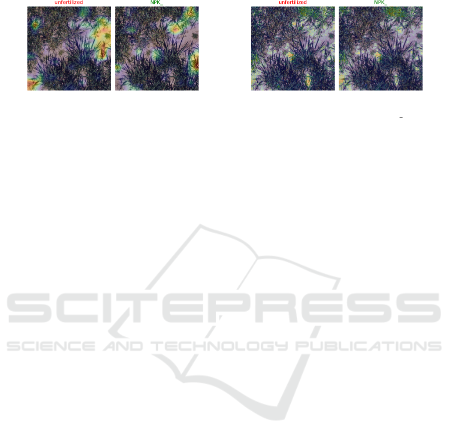
Figure 6: Visualization of the incorrect (red) and correct class (green) for two saliency maps. The label ”NPK ” correspond

to different nutrient statuses: nitrogen, phosphorous, and without potassium. Similar to the wood identiﬁcation dataset exper-

iment, GradCAM emphasizes distinct regions for each class, while full-backpropagation methods like Gradients tend to focus

on the same region for all classes.

Currently, the metrics rely primarily on intuitive rea-

soning and logical arguments, emphasizing the need

for further investigation to establish their soundness.

Figure 6 showcases the impact of visualizing the

saliency map for both incorrect and correct classes of

an image. In the case of the incorrect class assumption

where the plants were unfertilized, GradCAM pre-

dominantly emphasizes the soil. However, when as-

suming the plants are fertilized (correct class), Grad-

CAM shifts its focus towards the plants. On the other

hand, Gradients consistently highlights the plants for

both assumptions. This observation suggests that

Gradients may place greater importance on the dif-

ference in pixel value range between the two classes,

whereas GradCAM relies on distinct regions to de-

termine the class. Without knowing the ground truth

decision-making process, both approaches are possi-

ble.

5 DISCUSSION AND OUTLOOK

In this study, we conducted a comprehensive evalua-

tion of multiple state-of-the-art attribution maps using

real-world datasets from the agriculture and forestry

domains. Our analysis unveiled several crucial ﬁnd-

ings that shed light on the challenges and limitations

of these methods.

Firstly, we discovered a signiﬁcant lack of consis-

tency among attribution maps, both qualitatively and

quantitatively. Different methods often highlighted

different regions as important, resulting in inconsis-

tent region highlighting and excessive noise in certain

approaches. This inconsistency raises concerns about

the reliability and robustness of attribution maps for

interpreting neural network decisions in agriculture

and forestry tasks. We proposed two new metrics for

comparing the consistency of attribution maps: Pear-

son’s correlation coefﬁcient and Jensen-Shannon di-

vergence. Both metrics indicated weak agreement

among the maps.

Furthermore, when we compared the attribution

maps with expert annotations in the wood identiﬁca-

tion dataset, none of the maps showed high alignment

with expert annotations. This suggests that the neu-

ral network may learn different features from those

identiﬁed by human experts, highlighting a disparity

in the decision-making process. However, it is also

plausible that the maps themselves have limitations

in reﬂecting the true decision-making process of the

neural network.

Another important observation was the excessive

feature sharing across distinct classes in certain attri-

bution maps. This behavior can make it challenging

to interpret the results and uncover features that are

easily interpretable by humans. The ability to identify

unique features for each class is crucial for gaining a

better understanding of the decision-making process

of neural networks and providing meaningful expla-

nations.

Our evaluation of attribution maps using the met-

rics ”Insertion” and ”Deletion” showed certain lim-

itations. The parameters can have a signiﬁcant in-

ﬂuence on the results and the metrics are in general

not consistent across datasets. It is worth emphasiz-

ing that many CAMs (Wang et al., 2020a; Wang et al.,

2020b; Naidu et al., 2020) have asserted their superi-

ority based on the ”Insertion” and ”Deletion” metrics.

Given our ﬁndings, which highlight the unreliability

of these metrics, a question arises: Do these CAMs

genuinely demonstrate improvements compared to

GradCAM?

It is necessary to prove that the evaluation metrics

actually work. Otherwise, selecting the most suitable

attribution map for a speciﬁc task can only be based

on visual inspection and comparison with human an-

notation.

In conclusion, our research highlights the effec-

tiveness and reliability challenges of attribution maps

for wood species identiﬁcation and fertilizer treat-

VISAPP 2024 - 19th International Conference on Computer Vision Theory and Applications

490

ment classiﬁcation in the agriculture and forestry do-

mains. The lack of consistency among attribution

maps and the disparity between the maps and expert

annotations underscore the need for further research

and development in this ﬁeld. Future work should fo-

cus on developing improved attribution methods that

address the limitations identiﬁed in this study. Addi-

tionally, there is a necessity to ﬁnd metrics that can

objectively evaluate the attribution maps, as current

metrics such as ”Insertion” and ”Deletion” may lead

to conﬂicting results. By addressing these challenges,

we can enhance the interpretability and trustworthi-

ness of neural networks in critical applications within

agriculture and forestry.

REFERENCES

Ancona, M., Ceolini, E.,

Oztireli, A. C., and Gross,

M. H. (2017). A uniﬁed view of gradient-based at-

tribution methods for deep neural networks. CoRR,

abs/1711.06104.

Chattopadhay, A., Sarkar, A., Howlader, P., and Balasub-

ramanian, V. N. (2018). Grad-CAM++: Generalized

gradient-based visual explanations for deep convolu-

tional networks. In 2018 IEEE Winter Conference on

Applications of Computer Vision (WACV). IEEE.

Desai, S. and Ramaswamy, H. G. (2020). Ablation-cam: Vi-

sual explanations for deep convolutional network via

gradient-free localization. In 2020 IEEE Winter Con-

ference on Applications of Computer Vision (WACV),

pages 972–980.

Englebert, A., Cornu, O., and De Vleeschouwer, C. (2022).

Poly-cam: High resolution class activation map for

convolutional neural networks.

Fang, A., Kornblith, S., and Schmidt, L. (2023). Does

progress on ImageNet transfer to real-world datasets?

Fong, R., Patrick, M., and Vedaldi, A. (2019). Under-

standing deep networks via extremal perturbations

and smooth masks. CoRR, abs/1910.08485.

Fong, R. and Vedaldi, A. (2017). Interpretable explanations

of black boxes by meaningful perturbation. CoRR,

abs/1704.03296.

Fu, R., Hu, Q., Dong, X., Guo, Y., Gao, Y., and Li,

B. (2020). Axiom-based grad-cam: Towards accu-

rate visualization and explanation of cnns. CoRR,

abs/2008.02312.

Gomez, T., Fr

eour, T., and Mouch

ere, H. (2022). Metrics

for saliency map evaluation of deep learning explana-

tion methods. CoRR, abs/2201.13291.

He, K., Zhang, X., Ren, S., and Sun, J. (2015). Deep resid-

ual learning for image recognition.

Huang, G., Liu, Z., van der Maaten, L., and Weinberger,

K. Q. (2018). Densely connected convolutional net-

works.

Jiang, P.-T., Zhang, C.-B., Hou, Q., Cheng, M.-M., and Wei,

Y. (2021). Layercam: Exploring hierarchical class ac-

tivation maps for localization. IEEE Transactions on

Image Processing, 30:5875–5888.

Kapishnikov, A., Venugopalan, S., Avci, B., Wedin, B.,

Terry, M., and Bolukbasi, T. (2021). Guided inte-

grated gradients: An adaptive path method for remov-

ing noise. CoRR, abs/2106.09788.

Koch, G. and Koch, S. (2022). Holzartenwissen im app-

format : neue app ”macroholzdata” zur holzartenbes-

timmung und -beschreibung. Furnier-Magazin,

26:52–56.

Li, H., Li, Z., Ma, R., and Wu, T. (2022). Fd-cam: Improv-

ing faithfulness and discriminability of visual expla-

nation for cnns.

Liu, Z., Mao, H., Wu, C., Feichtenhofer, C., Darrell, T.,

and Xie, S. (2022). A convnet for the 2020s. CoRR,

abs/2201.03545.

Muhammad, M. B. and Yeasin, M. (2020). Eigen-cam:

Class activation map using principal components.

CoRR, abs/2008.00299.

Naidu, R., Ghosh, A., Maurya, Y., K, S. R. N., and

Kundu, S. S. (2020). IS-CAM: integrated score-

cam for axiomatic-based explanations. CoRR,

abs/2010.03023.

Nieradzik, L., Sieburg-Rockel, J., Helmling, S., Keuper,

J., Weibel, T., Olbrich, A., and Stephani, H. (2023).

Automating wood species detection and classiﬁcation

in microscopic images of ﬁbrous materials with deep

learning.

Omeiza, D., Speakman, S., Cintas, C., and Weldemariam,

K. (2019). Smooth grad-cam++: An enhanced infer-

ence level visualization technique for deep convolu-

tional neural network models. CoRR, abs/1908.01224.

Petsiuk, V., Das, A., and Saenko, K. (2018a). Rise: Ran-

domized input sampling for explanation of black-box

models.

Petsiuk, V., Das, A., and Saenko, K. (2018b). RISE: ran-

domized input sampling for explanation of black-box

models. CoRR, abs/1806.07421.

Poppi, S., Cornia, M., Baraldi, L., and Cucchiara, R. (2021).

Revisiting the evaluation of class activation mapping

for explainability: A novel metric and experimental

analysis. CoRR, abs/2104.10252.

Raatikainen, L. and Rahtu, E. (2022). The weighting game:

Evaluating quality of explainability methods.

Ribeiro, M. T., Singh, S., and Guestrin, C. (2016). ”why

should I trust you?”: Explaining the predictions of any

classiﬁer. CoRR, abs/1602.04938.

Richter, H. G. and Dallwitz (2000-onwards). Commercial

timbers: Descriptions, illustrations, identiﬁcation, and

information retrieval. (accessed on 15 May 2023).

Saporta, A., Gui, X., Agrawal, A., Pareek, A., Truong, S.

Q. H., Nguyen, C. D. T., Ngo, V.-D., Seekins, J.,

Blankenberg, F. G., Ng, A. Y., Lungren, M. P., and

Rajpurkar, P. (2022). Benchmarking saliency methods

for chest x-ray interpretation. Nature Machine Intelli-

gence, 4(10):867–878.

Selvaraju, R. R., Cogswell, M., Das, A., Vedantam, R.,

Parikh, D., and Batra, D. (2019). Grad-CAM: Visual

explanations from deep networks via gradient-based

Challenging the Black Box: A Comprehensive Evaluation of Attribution Maps of CNN Applications in Agriculture and Forestry

491

localization. International Journal of Computer Vi-

sion, 128(2):336–359.

Shi, X., Khademi, S., Li, Y., and van Gemert, J. (2020).

Zoom-cam: Generating ﬁne-grained pixel annotations

from image labels. CoRR, abs/2010.08644.

Simonyan, K., Vedaldi, A., and Zisserman, A. (2014).

Deep inside convolutional networks: Visualising im-

age classiﬁcation models and saliency maps. In Ben-

gio, Y. and LeCun, Y., editors, 2nd International

Conference on Learning Representations, ICLR 2014,

Banff, AB, Canada, April 14-16, 2014, Workshop

Track Proceedings.

Smilkov, D., Thorat, N., Kim, B., Vi

egas, F. B., and Wat-

tenberg, M. (2017). Smoothgrad: removing noise by

adding noise. CoRR, abs/1706.03825.

Springenberg, J. T., Dosovitskiy, A., Brox, T., and Ried-

miller, M. A. (2015). Striving for simplicity: The all

convolutional net. In Bengio, Y. and LeCun, Y., ed-

itors, 3rd International Conference on Learning Rep-

resentations, ICLR 2015, San Diego, CA, USA, May

7-9, 2015, Workshop Track Proceedings.

Sundararajan, M., Taly, A., and Yan, Q. (2017). Axiomatic

attribution for deep networks. CoRR, abs/1703.01365.

Szegedy, C., Vanhoucke, V., Ioffe, S., Shlens, J., and Wojna,

Z. (2015). Rethinking the inception architecture for

computer vision.

Tan, M. and Le, Q. V. (2019). Efﬁcientnet: Rethink-

ing model scaling for convolutional neural networks.

CoRR, abs/1905.11946.

Toda, Y. and Okura, F. (2019). How convolutional neural

networks diagnose plant disease. Plant Phenomics,

2019.

Wang, H., Naidu, R., Michael, J., and Kundu, S. S. (2020a).

Ss-cam: Smoothed score-cam for sharper visual fea-

ture localization.

Wang, H., Wang, Z., Du, M., Yang, F., Zhang, Z., Ding, S.,

Mardziel, P., and Hu, X. (2020b). Score-cam: Score-

weighted visual explanations for convolutional neural

networks.

Wheeler, E. A. (2004-onwards). Insidewood. (accessed on

15 May 2023).

Wheeler, E. A., Baas, P., Gasson, P. E., et al. (1989). Iawa

list of microscopic features for hardwood identiﬁca-

tion. Technical report.

Xu, S., Venugopalan, S., and Sundararajan, M. (2020). At-

tribution in scale and space. CoRR, abs/2004.03383.

Yi, J. (2023). CVPPA@ICCV’23: Image Classiﬁcation

of Nutrient Deﬁciencies in Winter Wheat and Winter

Rye.

Zeiler, M. D. and Fergus, R. (2013). Visualizing

and understanding convolutional networks. CoRR,

abs/1311.2901.

Zhang, J., Lin, Z., Brandt, J., Shen, X., and Sclaroff, S.

(2016). Top-down neural attention by excitation back-

prop. CoRR, abs/1608.00507.

Zhang, Q., Rao, L., and Yang, Y. (2021a). Group-cam:

Group score-weighted visual explanations for deep

convolutional networks. CoRR, abs/2103.13859.

Zhang, Y., Ti

no, P., Leonardis, A., and Tang, K. (2021b). A

survey on neural network interpretability. IEEE Trans-

actions on Emerging Topics in Computational Intelli-

gence, 5(5):726–742.

VISAPP 2024 - 19th International Conference on Computer Vision Theory and Applications

492