Dynamic Path Planning for Autonomous Vehicles Using Adaptive

Reinforcement Learning

Karim Wahdan

, Nourhan Ehab

, Yasmin Mansy

and Amr El Mougy

German University in Cairo, Cairo, Egypt

American University in Cairo, Cairo, Egypt

Keywords:

Dynamic Path Planning Autonomous Vehicles, Adaptive Reinforcement Learning.

Abstract:

This paper focuses on local dynamic path planning for autonomous vehicles, using an Adaptive Reinforcement

Learning Twin Delayed Deep Deterministic Policy Gradient (ARL TD3) model. This model effectively navi-

gates complex and unpredictable scenarios by adapting to changing environments. Testing, using simulations,

shows improved path planning over static models, enhancing decision-making, trajectory optimization, and

control. Challenges such as vehicle conﬁguration, environmental factors, and top speed require further reﬁne-

ment. The model’s adaptability could be enhanced by integrating more data and exploring a fusion between

supervised reinforcement learning and adaptive reinforcement learning techniques. This work advances au-

tonomous vehicle path planning by introducing an ARL TD3 model for real-time decision-making in complex

environments.

1 INTRODUCTION

Modern transportation systems are an essential cor-

nerstone of contemporary society, revolutionizing ur-

ban mobility and the efﬁcient movement of goods.

Yet, the increased utilization of these systems has

been accompanied by a surge in accident rates, a sig-

niﬁcant proportion of which can be attributed to hu-

man errors (Singh, 2017). In response to this chal-

lenge, the pursuit of fully autonomous transportation

has emerged as a promising solution. By reducing ac-

cidents and mitigating trafﬁc congestion, autonomous

vehicles hold the potential to transform transportation

systems fundamentally.

However, the realization of autonomous trans-

portation systems is not without its critical challenges.

One of the most threatening obstacles faced by cur-

rent autonomous systems is their ability to execute

real-time dynamic path planning in the face of unpre-

dictable environments. In these dynamic and ever-

changing scenarios, autonomous systems often strug-

gle to determine the optimal route and trajectory for

vehicles to navigate complex urban settings, avoid-

ing potential collisions in real-time. Traditional rule-

based systems and even earlier reinforcement learn-

ing methods have shown limitations in adapting to the

rapidly shifting conditions of the road (Sharma et al.,

2021).

This is precisely where Adaptive Reinforcement

Learning (ARL) takes center stage. ARL is a special-

ized subﬁeld of machine learning and reinforcement

learning, uniquely designed to create autonomous

systems that possess the capacity to adapt their behav-

ior and decision-making processes in response to real-

time changes in their environment (Li et al., 2021). In

the context of autonomous vehicles, ARL becomes a

critical enabler, as it allows these vehicles to contin-

ually reﬁne their policies, optimizing their decision-

making in complex and uncertain trafﬁc situations.

The need for ARL in the development of autonomous

vehicles stems from the dynamic and unpredictable

nature of real-world trafﬁc environments. Unlike tra-

ditional rule-based systems or static reinforcement

learning, ARL algorithms can adapt to unexpected oc-

currences, rapidly shifting trafﬁc patterns, and diverse

driving conditions. These models are robust to uncer-

tainties, less likely to fall victim to biases, and can

learn efﬁciently even with limited data, making them

well-suited for real-world applications.

The objective of this research is to harness the

potential of ARL models for dynamic path planning

in autonomous systems, speciﬁcally autonomous ve-

hicles. We aim to create a ﬂexible model that can

adapt seamlessly to evolving environmental condi-

tions. This adaptability not only enhances the navi-

gational capabilities of autonomous vehicles but also

272

Wahdan, K., Ehab, N., Mansy, Y. and El Mougy, A.

Dynamic Path Planning for Autonomous Vehicles Using Adaptive Reinforcement Learning.

DOI: 10.5220/0012363300003636

Paper published under CC license (CC BY-NC-ND 4.0)

In Proceedings of the 16th International Conference on Agents and Artiﬁcial Intelligence (ICAART 2024) - Volume 1, pages 272-279

ISBN: 978-989-758-680-4; ISSN: 2184-433X

minimizes data requirements and reduces the impact

of biases. In our evaluation, we place signiﬁcant em-

phasis on metrics such as control smoothness and suc-

cess rate to provide a comprehensive assessment of

real-world performance. Our ultimate goal is to con-

tribute to the ongoing evolution of autonomous trans-

portation systems, thereby advancing their capacity

for real-time decision-making in ever-changing envi-

ronments and enhancing the safety and efﬁciency of

our transportation networks, all while highlighting the

pivotal role of ARL in this endeavor.

The rest of this paper is structured as follows. Sec-

tion 2 presents the design and implementation of our

ARL model for dynamic path planning. Section 3 un-

veils the speciﬁc evaluation metrics and testing sce-

narios employed, presenting their corresponding re-

sults. Section 4 presents the analysis of these results,

discusses their implications, and draws comparisons

with other related work in the ﬁeld. Finally, Section 5

presents some concluding remarks.

2 PROPOSED FRAMEWORK

DESIGN

In the pursuit of developing advanced dynamic path

planning for autonomous vehicles, our paper intro-

duces a comprehensive framework that leverages the

power of Adaptive Reinforcement Learning (ARL).

This section provides a detailed overview of this

framework, which is divided into three main com-

ponents: the Meta-Drive simulation environment, the

TD3 model and its policy, and an adaptive module.

2.1 Framework Overview

The core of our approach lies in the interaction be-

tween three central components: the Meta-Drive sim-

ulation environment, the TD3 model and its policy,

and the adaptive module. Figure 1 is a visualization

of those interactions.

The Meta-Drive environment (Li et al., 2022)

stands as a robust simulation platform, purpose-built

for the training and evaluation of Reinforcement

Learning (RL) autonomous vehicles within intricate

urban trafﬁc environments. With its high ﬁdelity and

realistic features, including an accurate physics en-

gine, diverse vehicle dynamics, and realistic trafﬁc

patterns, Meta-Drive provides an exceptional setting

for training autonomous vehicles.

At the heart of our framework, the Twin Delayed

Deep Deterministic Policy Gradients (TD3) model

plays a pivotal role in policy development and action

Figure 1: Framework Overview.

generation. Informed by observations from the Meta-

Drive environment, the TD3 model formulates actions

to be executed by autonomous vehicles. The policy

embedded within the TD3 model guides the process

of action selection.

Finally, the MetaDrive environment not only sup-

plies observation states and receives actions from the

TD3 model but also provides rewards for the ac-

tions taken, serving as a feedback signal for learning.

Additionally, it shares crash information for speciﬁc

episodes with the adaptive module, allowing it to initi-

ate new training cycles as necessary. In what follows,

we delve into the details of each module.

2.2 Meta-Drive Environment

The Meta-Drive (Li et al., 2022) is a driving simula-

tion platform that provides observations with a wide

range of sensory input including low-level sensors LI-

DAR and depth camera, and high-level scene infor-

mation such as the road environment, nearby vehicles,

and vehicle status. Our observation space can be di-

vided into three main sections: the vehicle state, nav-

igation information, and surrounding data. The vehi-

cle state variables are 19 values including values like

steering, heading, and velocity. The navigation infor-

mation variables are 10 values that represent the rela-

tionship between the vehicle and its ﬁnal destination

and following checkpoints The surrounding informa-

tion is a vector that captures various aspects of the en-

vironment, including data from 2 side detectors, and

40 LIDAR points input.

In our context, the action space comprises two es-

sential components: steering and throttle. These com-

ponents are assigned numerical values that span from

-1 to 1. This numerical range facilitates precise and

adaptable maneuvering in various driving scenarios.

The reward function in Meta-Drive is designed to

Dynamic Path Planning for Autonomous Vehicles Using Adaptive Reinforcement Learning

273

incentivize desirable behaviors and discourage unde-

sirable ones. It is be deﬁned as:

R(s,a,s

) = c

· Driving reward + c

· Speed reward

+ Termination reward

The driving reward is calculated as d(t +1)−d(t),

where d(t + 1) and d(t) denote the longitudinal co-

ordinates of the target vehicle. with c

= 1 The

speed reward is calculated asv

max

, which encour-

ages the agent to maintain a high speed while min-

imizing unnecessary accelerations and decelerations.

with c

= 0.1

The termination reward is given to the au-

tonomous vehicle at the end of the episode, based on

the termination state. That can be a success reward

(a positive reward), an out-of-road penalty, a crashed-

vehicle penalty, or a crashed-object penalty — all of

which are negative.

There is one additional optional parameter that we

introduced to the reward function called the ”lateral

reward”. This is a multiplier that is added to the driv-

ing reward to incentivize the agent to stay in lane. The

lateral reward is used on some models in testing

2.3 TD3 Model Development

The TD3 model serves as the fundamental component

of our adaptive reinforcement learning (ARL) solu-

tion. It is a signiﬁcant advancement over the tradi-

tional policy of the Gradient actor-critic and DDPG

model by enhancing the error approximation associ-

ated with the Actor-Critic models through the incor-

poration of twin critics. This effectively mitigates

the issue of the overestimation bias commonly ob-

served and a delayed policy update mechanism en-

abling a more precise estimation of values and target

policy smoothing. Consequently, this encourages ex-

ploration and prevents the policy from becoming too

deterministic by incorporating noise during the train-

ing phase.

2.3.1 Replay Buffer

The ﬁrst component of our model is the replay buffer,

which serves as the main memory of the reinforce-

ment learning model and is utilized to store and sam-

ple past experiences, allowing the model to draw from

its accumulated experiences to generate training data

for efﬁcient learning. Our replay buffer is imple-

mented with a ﬁxed capacity, to prevent the model

from being inﬂuenced by ancient data in new training

cycles, allowing it to be more dynamic in new envi-

ronments. Each transition represents the change of

state based on the actions of the autonomous vehicle

and is stored in the replay buffer as ﬁve components:

the current state, the resulting next state, the action

taken, the associated reward, and an episode comple-

tion indicator.

The initialized replay buffer comprises a data

structure of a predetermined size, featuring an indica-

tor pointing to either the subsequent vacant position

or the position earmarked for replacement.

Transitions can be added to the replay buffer and

they are added to the next vacant position or the oldest

transition is replaced with the newest.

Any sample subset of the replay buffer can be gen-

erated for training the model on a subset of previous

experiences.

2.3.2 Neural Networks Infrastructure

The model consists of six dense deep neural networks

each with their functionality, the actor-network serves

as the policy network, responsible for generating ac-

tions based on the current state of the environment.

The critic-networks play a crucial role in esti-

mating the action-value function, which evaluates the

quality of the actions taken by the actor-network, the

critic-networks output a scalar value that represents

the estimated action-value or Q-value for the given

state-action pair.

To stabilize the training process and enhance the

overall performance of the TD3 model, the introduc-

tion of two sets of target networks is crucial. These

networks include the target actor-network and the

target-critic networks, which play integral roles in es-

timating action values and reducing overestimation

bias.

The target actor-network and target critic-

networks are replicas of their respective actor and

critic networks. They do not get updated during

training; instead, their parameters change gradually

through soft target network updates. This process in-

volves smoothly blending the target network’s param-

eters with those of the actual network, using a small

factor to achieve a gradual update. Soft target net-

work updates are crucial for stabilizing the learning

process.

2.3.3 TD3 Mechanisms

The TD3 model follows a comprehensive training ap-

proach, involving actions like sampling transitions,

computing target Q-values, minimizing overestima-

tion bias, and employing soft target network updates.

These mechanisms collectively enable precise value

estimation, enhanced exploration, and stabilization of

the learning process.

ICAART 2024 - 16th International Conference on Agents and Artiﬁcial Intelligence

274

The intricacies of the TD3 model and its training

process are encapsulated in a single entity, as demon-

strated in Algorithm 2. This entity efﬁciently orches-

trates the model’s interactions with its environment,

facilitating learning, and adaptation.

Data: state dim, action dim, max action

Result: TD3 Agent

Function TD3(state dim, action dim,

max action)

Initialize actor, actor target, critic, and

critic target networks;

Load actor, critic weights into actor target,

critic target;

Initialize actor and critic optimizer;

Set maximum action value;

Function select action(state)

return actor(state);

Function train(replay buffer,

iterations, batch size, discount,

tau, policy noise, noise clip,

policy freq)

for it ← 1 to iterations do

Sample transitions (s, s’, a, r, d);

From the next state s’, compute the

next action a’ using actor target;

Add Gaussian noise to the next action

and clamp it;

Compute target Q-values using the two

critic targets;

Keep the minimum of these two

Q-values: min(Qt1, Qt2);

Compute target Q-values with discount

factor;

Compute current Q-values using two

critic networks;

Compute critic loss;

Backpropagate the Critic loss and

update the parameters of the two

Critic models using SGD optimizer;

if it % policy freq == 0 then

Compute actor loss;

Update actor parameters using

gradient ascent optimizer;

Update actor target and critic target

weights using Polyak averaging

every two iterations;

end

Function save(filename, directory)

Save actor, critic weights to a ﬁle;

Function load(filename, directory)

Load actor, critic weights from a ﬁle;

Algorithm 1: TD3 Class.

2.3.4 Model Training

The training process unfolds over millions of

timesteps, driven by a robust training loop. The key

steps in the training loop encompass episode monitor-

ing, policy evaluation, reward calculation, and storage

of evaluation results. These iterative steps ensure that

the agent continuously reﬁnes its policy through in-

teractions, training, and evaluations within the envi-

ronment.

At each timestep, the procedure checks if the

episode has ended or if the maximum steps per

episode have been reached. If so, training begins.

Using experiences from the replay buffer, the pol-

icy is learned with the train() function, but only

if there are enough experiences and it’s not the ﬁrst

timestep. After training, the current policy is eval-

uated with the evaluate_policy() function, based

on the eval_freq argument. The evaluation results

are stored, and the policy is saved.

The evaluate_policy() function takes a given

model and ”n” episodes to test it on each episode con-

sisting of ”m” steps and then returns the average re-

ward over testing and the average number of steps per

episode before termination. In our train the models

were tested on 10 episodes of 10e4 steps each. again

these values were obtained through multiple iterations

of tuning of trying to ensure a steady reward output of

the same model.

Episode-related variables are updated, timesteps

increase, and the environment state resets. The agent

decides whether to explore (before start timesteps)

or choose an action based on the learned policy. If

there’s exploration noise, it adds noise to the ac-

tion within action space boundaries. The chosen ac-

tion is executed in the environment, and the code re-

trieves the next observation, reward, and episode sta-

tus. Episode and overall rewards are updated, and the

transition is stored in the replay buffer.

Once the main loop ends, the ﬁnal policy evalu-

ation is added to the evaluations list, and if the save

models ﬂag is set, the policy is stored. The ﬁnal

evaluation result is saved as well. The environment

is closed and restarted. The average reward across

episodes is computed by dividing the total reward by

the number of episodes (episode num). This loop it-

eratively improves the agent’s policy through interac-

tions, training, and periodic evaluations with the en-

vironment.

2.4 Adaptive Module

The ﬁnal piece of our framework is the adaptive mod-

ule, a hybrid approach that combines batch learn-

Dynamic Path Planning for Autonomous Vehicles Using Adaptive Reinforcement Learning

275

ing and online learning to maximize adaptability. It

begins with an ofﬂine training phase in which the

model calculates an average reward across all training

episodes. This average reward serves as a threshold

for subsequent episodes.

During new episodes, if the model’s performance

falls below 20% of the average reward, it triggers

an online learning session, indicating a signiﬁcant

environmental change. If, during three consecutive

episodes, the model scores below 70% of the average

reward, it initiates another online training session, ad-

dressing more subtle changes in the environment.

To ensure continual adaptability, the model en-

gages in batch learning cycles every 10

timesteps,

enabling it to remain up-to-date with evolving trends

and environmental shifts. This hybrid incremen-

tal/batch adaptive learning approach enhances the

model’s capacity to adapt to both signiﬁcant and

subtle changes in the environment, making it well-

equipped to handle dynamic, complex trafﬁc scenar-

ios.

The parameters of 20%, 70%, and 10

steps were

derived through multiple sessions of hyperparameter

tuning by trying multiple permutations of values for

each parameter.

3 RESULTS

To test the effectiveness of our proposed model, rigor-

ous tests on 5 different challenging real-world urban

scenarios were performed. Each is designed to test an

aspect of the model’s performance. Four distinct TD3

models, each with variations in training type, train-

ing duration, and the presence of lateral reward were

tested.

3.1 Scenarios and Model Variations

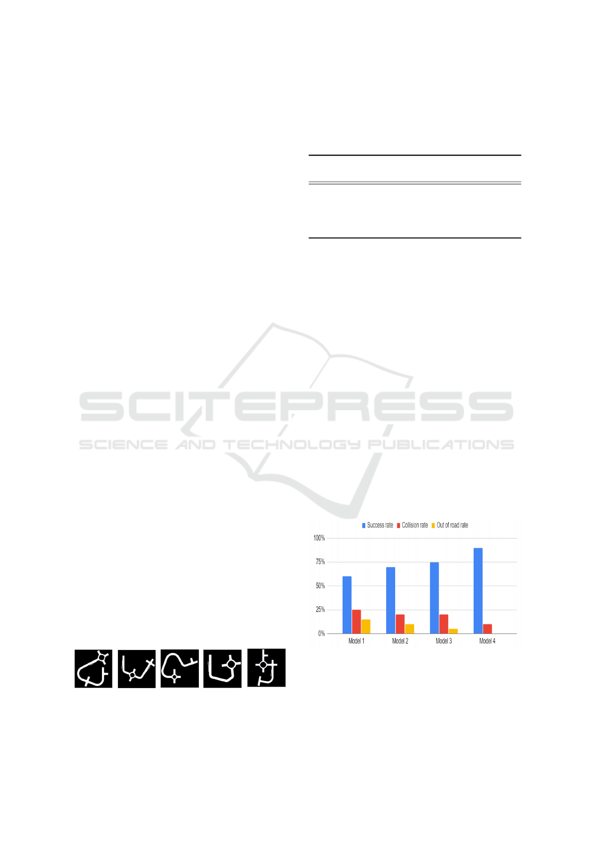
Figure 2 Represents a top overview of each of the 5

distinct maps that models were tested on, tests include

high trafﬁc density, complex road layouts, and diverse

lane conﬁgurations. This diversity ensures a compre-

hensive assessment of the models’ adaptability to var-

ious urban settings. a detailed description of each sce-

nario will be provided in the corresponding scenario

result’s sub-section

Figure 2: Scenarios Maps Overview.

Table 1 shows a comparison between the attributes

and distinguishing features of the four models sub-

jected to testing which can be elaborated upon as fol-

lows:

Table 1: Model Performance Summary.

Model Training

Type

Duration Lateral

Reward

Model 1 Static 10

Model 2 Static 2 ∗ 10

Model 3 Adaptive 10

Yes

Model 4 Adaptive 2 ∗ 10

Yes

3.2 Scenario 1

In the ﬁrst scenario, the models face a map with six

blocks. The environment is conﬁgured with a trafﬁc

density of 0.1, representing a moderate level of trafﬁc.

The lanes on the roads are randomly assigned, and the

vehicle spawn lane is randomized.

As Illustrated by ﬁgure 3 the performance of the

four models on this map. Model 1 achieved a 60%

success rate, indicating a moderate level of compe-

tence in completing driving tasks. However, it had a

higher collision rate of 25% and a 15% out-of-road

rate. Model 2 showed improvement with a 70% suc-

cess rate, a lower collision rate of 20%, and a reduced

out-of-road rate of 10%. Model 3 displayed further

improvement, achieving a 75% success rate, match-

ing Model 2’s collision rate while signiﬁcantly reduc-

ing out-of-road incidents to 5%. The top-performing

model in this scenario was Model 4, with an impres-

sive 90% success rate, excellent collision avoidance

(10% collision rate), and perfect adherence to the des-

ignated road path (0% out-of-road rat

Figure 3: Scenario 1 Results.

ICAART 2024 - 16th International Conference on Agents and Artiﬁcial Intelligence

276

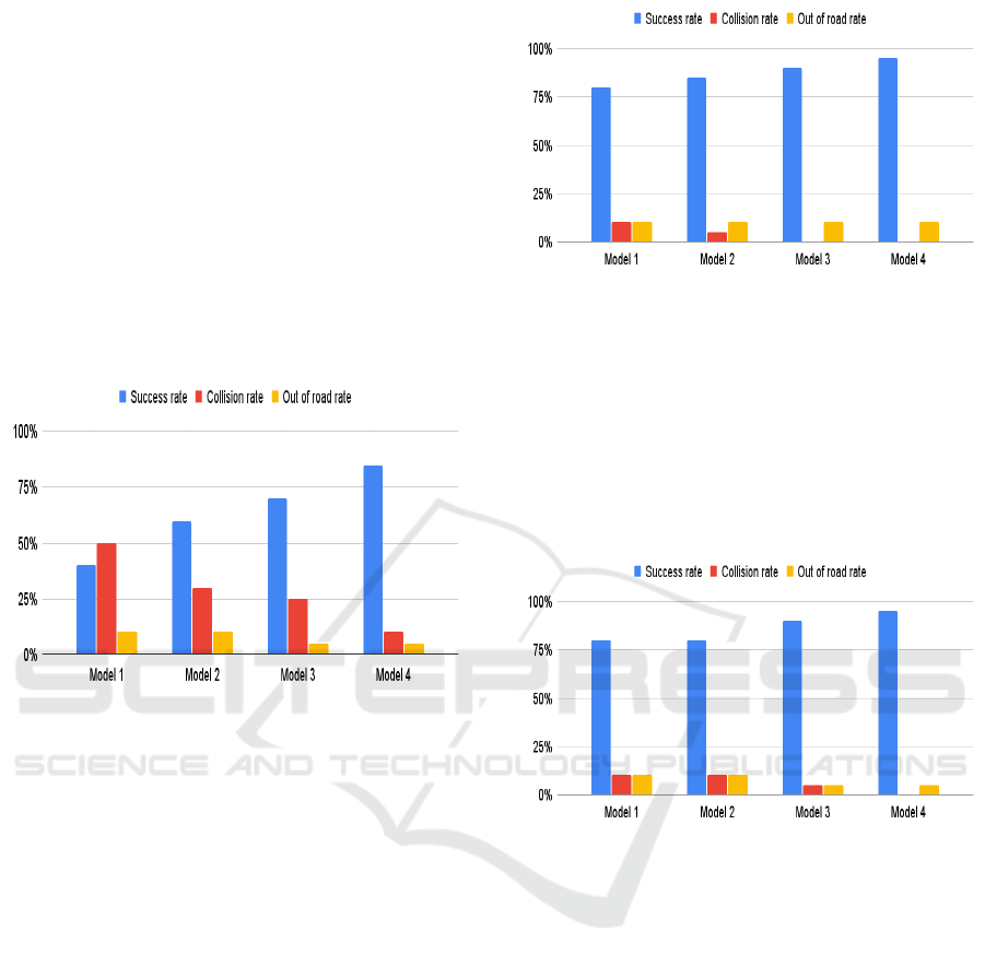
3.3 Scenario 2

In the second scenario, the models are tested on a map

with six blocks, featuring a higher trafﬁc density of

0.4, representing heavy trafﬁc. The lanes on the roads

are randomly assigned, and the vehicle spawn lane is

randomized.

As Illustrated by ﬁgure 4 All Models had slightly

worse performance than scenario 1 due to it being a

challenging scenario with a more complex conﬁgura-

tion of blocks and higher trafﬁc density Model 4 had

the best performance by quite a large margin while

model 1 had the worst performance. while model 3

slightly outperformed model 2.

Figure 4: Scenario 2 Results.

3.4 Scenario 3

In the third scenario, the models face a map with six

blocks and a trafﬁc density of 0.1, similar to Scenario

1. However, the number of lanes on the roads is as-

signed to three lanes, and the vehicle spawn lane is

also randomized.

As Illustrated by ﬁgure 5 All Models had signiﬁ-

cantly better performance than scenario 1,2 due to it

being a simple scenario with a less complex conﬁgu-

ration of blocks, lower trafﬁc density, and a known

number of lanes The highest-performing model re-

mained Model 4 with its success rate at 90% while

model 1 had the worst performance. while model 3

slightly outperformed model 2.

3.5 Scenario 4

Scenario 4 presents a map with six blocks and a traf-

ﬁc density of 0.1, mirroring Scenario 3. However, in

this scenario, the lanes on the roads are assigned to

three lanes, and the vehicle spawn lane is placed in

the middle lane.

As Illustrated by ﬁgure 6 All Models had the best

Figure 5: Scenario 3 Results.

performance due to it being a simple scenario with

a less complex conﬁguration of blocks lower trafﬁc

density and a known number of lanes and spawning

point Model 4 had the best performance by quite a

large margin with a success rate of 95% while model

1 had the worst performance with a success rate of

about 80%. while model 3 slightly outperformed

model 2.

Figure 6: Scenario 4 Results.

3.6 Scenario 5

In this scenario, the four models are tested on the ﬁfth

map, which consists of 7 blocks. The environment is

conﬁgured with a trafﬁc density of 0.7, meaning that

there is a moderate amount of trafﬁc on the roads. The

lanes in the environment roads are randomly assigned

and the vehicle spawn lane is also randomized.

As Illustrated by ﬁgure 7 All Models had the worst

performance due to it being a simple scenario with a

more complex conﬁguration of ”7” blocks, and higher

trafﬁc density. Model 4 had the best performance by

quite a large margin with a success rate of 85% while

model 1 had the worst performance with a success

rate of about 50%. while model 3 slightly outper-

formed model 2.

Dynamic Path Planning for Autonomous Vehicles Using Adaptive Reinforcement Learning

277

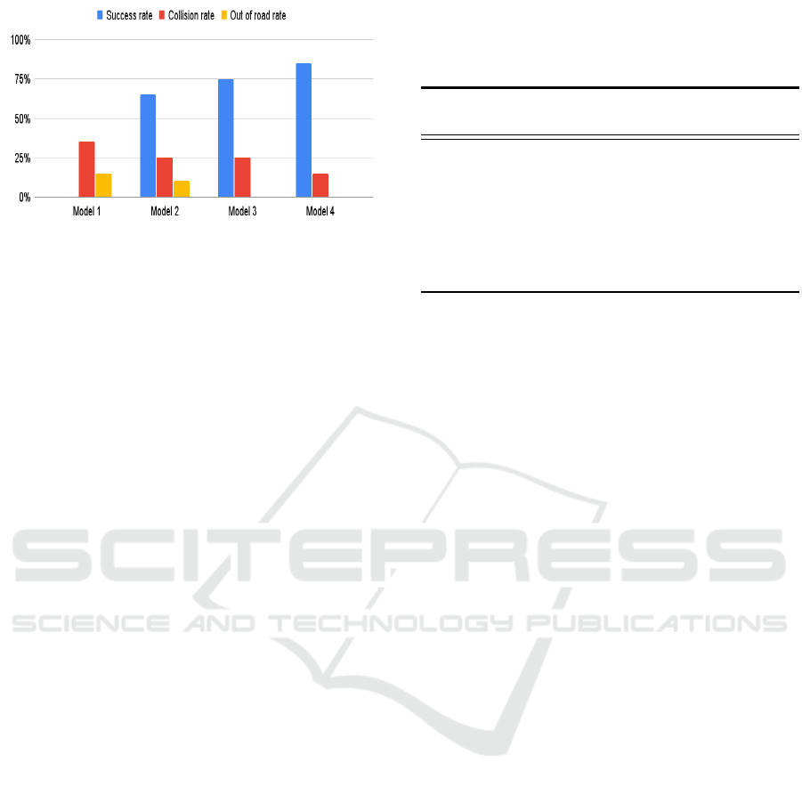
Figure 7: Scenario 5 Results.

4 DISCUSSION

The evaluation of the four models in realistic urban

environments provided valuable insights into their

performance, accuracy, and adaptability. The compar-

ison of metrics across different scenarios sheds light

on the strengths and weaknesses of each model con-

ﬁguration.

4.1 Model Performance and Accuracy

The adaptive TD3 models (Models 3 and 4) consis-

tently outperformed the static TD3 models (Models 1

and 2) in all scenarios. They showed higher success

rates, lower collision rates, and better adherence to

trafﬁc rules, indicating their effectiveness in handling

dynamic urban scenarios.

Model 4 outperformed all other models across var-

ious scenarios, achieving the highest success rate in

urban driving. Its success can be attributed to adap-

tive training, longer training duration, and the inclu-

sion of a lateral reward component. This model ex-

celled in collision avoidance and adherence to trafﬁc

rules, making it the preferred choice for real-world

urban driving.

Model 3 also performed well, with success rates

comparable to Model 4. This highlights the signiﬁ-

cance of adaptive elements in reinforcement learning

models for urban driving.

In contrast, Models 1 and 2, which employed

static training, exhibited lower success rates and

higher collision rates due to their inability to adapt to

changing conditions. While Model 2 performed bet-

ter than Model 1, both lagged behind adaptive mod-

els, underscoring the limitations of static training for

handling complex urban driving scenarios.

Furthermore, Models 3 and 4 demonstrated im-

proved steering control smoothness, thanks to their

adaptability and continuous learning during testing.

This improvement in steering control contributed to

their higher success rates and better adherence to traf-

ﬁc rules.

Table 2: Model Performance Summary.

Model Success

Rate

Collision

Rate

Steering

Control

Model 1 Low High Not

Smooth

Model 2 Moderate Moderate Not

Smooth

Model 3 Above

Model 2

Moderate Improved

Model 4 Highest Low Improved

4.2 Training Time and Average Reward

The training time and average reward achieved dur-

ing the training phase were analyzed, revealing some

noteworthy ﬁndings. Models 2 and 4, beneﬁting

from longer training durations of 2 ∗ 10

steps, out-

performed Models 1 and 3 in terms of average re-

ward. This highlights the positive correlation between

extended training time and improved training perfor-

mance, resulting in higher rewards.

However, it’s crucial to consider that longer train-

ing durations come with increased computational re-

source requirements and time investments. Therefore,

there exists a trade-off between training time and per-

formance, as shown in Model 3 performance, despite

having a shorter training duration of 10

steps, still

delivered impressive performance and accuracy. This

indicates that adaptive training techniques can effec-

tively optimize training efﬁciency, allowing compet-

itive results to be achieved within a reasonable time

frame.

4.3 Related Work

In the realm of local path planning for autonomous

vehicles in dynamic environments, research has iden-

tiﬁed limitations in classical algorithms for real-

time adaptability, as discussed by (Gonzalez Bautista

et al., 2015). In contrast, our Adaptive Reinforce-

ment Learning (ARL) model excels in swift decision-

making in rapidly changing situations.

Another study by (Panda et al., 2020) found ex-

isting algorithms lacking in reliability for Automated

Underwater Vehicles (AUVs) in unmapped environ-

ments. Our model addresses this challenge with an

adaptive module for effective adaptation in unmapped

territories over time.

In a different study, (Hebaish et al., 2022) in-

troduced a fusion method combining Twin Delayed

ICAART 2024 - 16th International Conference on Agents and Artiﬁcial Intelligence

278

Deep Deterministic (TD3) and Supervised Learning

(SL) to reduce training time and improve success rates

in speciﬁc scenarios.

Our model surpasses this approach and results in

even more complex scenarios with multiple lanes and

variable spawning positions, thanks to ﬁne-tuning and

its adaptive module.

Additionally, (Zhou et al., 2022) extended the

work of (Gonzalez Bautista et al., 2015) by exploring

various machine learning techniques and highlighting

the time-consuming nature of training RL policies.

Our model builds upon the TD3 model by continu-

ously updating its policy and adapting to new data

without extensive training or concept drift concerns.

5 CONCLUSION

The Adaptive TD3 model introduced shows a promis-

ing solution to the complex problem of local dy-

namic path planning in autonomous driving. It builds

upon the foundation of the classical TD3 model and

aims to address the real-world challenges faced by

autonomous vehicles. The results of our evaluation

demonstrate the model’s superior performance in var-

ious scenarios, emphasizing its adaptability and effec-

tiveness.

However, it is important to acknowledge several

key limitations. The model’s maximum velocity con-

straint of 40 km/h, while necessary for stability within

the limited training time, is a signiﬁcant drawback.

Future research should focus on developing methods

to raise the speed limit without compromising perfor-

mance, allowing the model to operate effectively at

higher speeds.

Another limitation is the lengthy training period,

especially at low speeds. This highlights the need for

more efﬁcient training techniques that can expedite

the learning process. One potential solution is the in-

tegration of Adaptive Reinforcement Learning (ARL)

with Supervised Reinforcement Learning (SRL) to

create an ASRL TD3 model, offering faster and more

effective training.

Environmental factors, such as weather condi-

tions, lighting variations, and interactions with pedes-

trians, were not considered in the evaluation. These

factors play a crucial role in real-world driving scenar-

ios, and future research should focus on incorporating

them into the model’s input and training process. Ad-

dressing these aspects is vital for enhancing the real-

world applicability of the Adaptive TD3 model.

REFERENCES

Gonzalez Bautista, D., P

erez, J., Milanes, V., and

Nashashibi, F. (2015). A review of motion planning

techniques for automated vehicles. IEEE Transactions

on Intelligent Transportation Systems, 17:1–11.

Hebaish, M. A., Hussein, A., and El-Mougy, A. (2022).

Supervised-reinforcement learning (srl) approach for

efﬁcient modular path planning. In 2022 IEEE 25th

International Conference on Intelligent Transporta-

tion Systems (ITSC), pages 3537–3542.

Li, Q., Peng, Z., Feng, L., Zhang, Q., Xue, Z., and Zhou, B.

(2022). Metadrive: Composing diverse driving sce-

narios for generalizable reinforcement learning. IEEE

Transactions on Pattern Analysis and Machine Intel-

ligence.

Li, X., Xu, H., Zhang, J., and Chang, H.-h. (2021). Opti-

mal hierarchical learning path design with reinforce-

ment learning. Applied psychological measurement,

45(1):54–70.

Panda, M., Das, B., Subudhi, B., and Pati, B. B. (2020). A

comprehensive review of path planning algorithms for

autonomous underwater vehicles. International Jour-

nal of Automation and Computing.

Sharma, O., Sahoo, N. C., and Puhan, N. B. (2021). Recent

advances in motion and behavior planning techniques

for software architecture of autonomous vehicles: A

state-of-the-art survey. Engineering applications of

artiﬁcial intelligence, 101:104211.

Singh, S. K. (2017). Road trafﬁc accidents in india: is-

sues and challenges. Transportation research proce-

dia, 25:4708–4719.

Zhou, C., Huang, B., and Fr

anti, P. (2022). A review of mo-

tion planning algorithms for intelligent robots. Jour-

nal of Intelligent Manufacturing, 33(2):387–424.

Dynamic Path Planning for Autonomous Vehicles Using Adaptive Reinforcement Learning

279