Decoupling the Backward Pass Using Abstracted Gradients

Kyle Rogers

1,∗ a

, Hao Yu

1,∗ b

, Seong-Eun Cho

2 c

, Nancy Fulda

1 d

, Jordan Yorgason

3 e

and Tyler J. Jarvis

2 f

Department of Computer Science, Brigham Young University, Provo, Utah, U.S.A.

Department of Mathematics, Brigham Young University, Provo, Utah, U.S.A.

Cellular Biology and Physiology, Center for Neuroscience, Brigham Young University, Provo, Utah, U.S.A.

Keywords:

Machine Learning, Matrix Abstraction, Biologically Inspired Learning Algorithm, Model Parallelization,

Network Modularization, Backpropagation, Skip Connections, Neuromorphic.

Abstract:

In this work we introduce a novel method for decoupling the backward pass of backpropagation using math-

ematical and biological abstractions to approximate the error gradient. Inspired by recent ﬁndings in neuro-

science, our algorithm allows gradient information to skip groups of layers during the backward pass, such that

weight updates at multiple depth levels can be calculated independently. We explore both gradient abstrac-

tions using the identity matrix as well as an abstraction that we derive mathematically for network regions that

consist of piecewise-linear layers (including layers with ReLU and leaky ReLU activations). We validate the

derived abstraction calculation method on a fully connected network with ReLU activations. We then test both

the derived and identity methods on the transformer architecture and show the capabilities of each method on

larger model architectures. We demonstrate empirically that a network trained using an appropriately chosen

abstraction matrix can match the loss and test accuracy of an unmodiﬁed network, and we provide a roadmap

for the application of this method toward depth-wise parallelized models and discuss the potential of network

modularization by this method.

1 INTRODUCTION

There are numerous types of deep neural networks

which excel on various tasks, but they heavily rely

on a rigid error backpropagation procedure. From

multilayer perceptrons to convolutional neural nets to

transformer-based architectures, these models com-

pute the gradient of the loss with respect to each

model parameter to ﬁnd a local minimum on the

model’s loss surface. Gradient computation is an ex-

pensive process and requires the gradient to be calcu-

lated layerwise backward through the neural network.

This learning paradigm is incredibly successful, but

also inﬂexible as gradient computation requires dif-

ferentiable operations and sequential processing of

data through the network.

https://orcid.org/0000-0001-8494-5121

https://orcid.org/0009-0003-5106-6042

https://orcid.org/0009-0003-3416-461X

https://orcid.org/0000-0001-9391-8301

https://orcid.org/0000-0002-5687-0676

https://orcid.org/0000-0002-3767-029X

∗

These authors contributed equally

In this work we present a new tool, termed ab-

straction matrices, which enable gradient information

to be passed backward to multiple locations in the net-

work in a decoupled fashion. We show that break-

ing up the backward pass in this way does not hinder

model performance and allows more ﬂexibility during

backpropagation. Given this result, we explore sev-

eral implications of our method: 1) theoretical depth-

wise model parallelization, 2) network modulariza-

tion, and 3) algorithm innovation.

Our method introduces a set of matrices

,...,M

} which correspond to the abstracted

network regions. These matrices are calculated dur-

ing each forward pass in such a way that, when M

multiplied by gradient information from the network

layer immediately following the kth abstracted

region, the result is a reasonable approximation of the

gradient information which would have been passed

to the preceding layer via traditional backpropagation

methods. Said another way, during the backward

pass, the abstraction matrices {M

,...,M

} are used

to quickly transmit error information backward across

multiple layer blocks via a simple matrix multiplica-

Rogers, K., Yu, H., Cho, S., Fulda, N., Yorgason, J. and Jarvis, T.

Decoupling the Backward Pass Using Abstracted Gradients.

DOI: 10.5220/0012362800003636

Paper published under CC license (CC BY-NC-ND 4.0)

In Proceedings of the 16th International Conference on Agents and Artiﬁcial Intelligence (ICAART 2024) - Volume 3, pages 507-518

ISBN: 978-989-758-680-4; ISSN: 2184-433X

507

tion rather than via more complex backpropagation

calculations.

The biological inspiration for this method, which

both motivates and, to an extent, justiﬁes the use of

imperfect gradient approximation in lieu of rigorously

calculated gradients, lies in observed ﬁndings from

foundational neuroscience studies that identiﬁed feed-

back signals in biological brains are backpropagated

both through localized synaptic retrograde signalling

and through shortened feedback loops to distant lay-

ers (Seger and Miller, 2010; Sesack and Grace, 2010).

The synaptic updates are more precise, whereas the

shortened feedback loops are less accurate but facil-

itate a faster training response because they bypass

many of the intervening neurons (Gerdeman et al.,

2002; Alger, 2002). These biological foundations

provide both the inspiration and a motivating prece-

dent for our study of approximate signal mediation

via abstraction matrices.

The contributions of this paper are as follows: (a)

We present a biologically inspired paradigm for neu-

ral network training based on abstracted gradient in-

formation mediated via simple matrix multiplications

(Sections 3.1 and 3.2); (b) We present a justiﬁca-

tion for a least-squares method for computing abstrac-

tion matrices {M

,...,M

} in the case that the cor-

responding layers are comprised of piecewise-linear

functions; (c) We introduce a simpliﬁcation paradigm

= I ∀k that reduces calculation overhead and is

rooted in biological precedents (Section 3.4); (d) We

validate the effectiveness of abstraction matrices in

both multilayer perception and transformer architec-

tures, and show that the abstraction of layer blocks

via M

can be achieved without a drop in training ac-

curacy (Sections 4.1 and 4.2); (e) We examine antici-

pated speedups that could be obtained by implement-

ing our abstracted architecture in a fully parallelized

environment (Section 5.1): and (d) we discuss the ap-

plication of our method in algorithm innovation and

network modularization (Section 5.2).

2 RELATED WORK

Incomplete Gradient-Based Learning: Computing

the error gradient with respect to model parameters

is, in its pure form, a prohibitively intensive pro-

cess. True gradient descent involves iterating through

the entire dataset, computing each weight’s gradi-

ent with respect to calculated error, and then updat-

ing the parameters in proportion to the learning rate.

This is highly impractical, and thus gradients are usu-

ally computed for only a subset of the data at a time

(Amari, 1993). Despite using only an approximation

of the true gradient, SGD methods have proved to be

quite effective in training neural networks in a super-

vised manner. Our work builds on this precedent by

using abstraction matrices to quickly transmit approx-

imations of the calculated error gradient.

Further approximations of the error gradient

have been utilized to implement layer-parallelization

unther et al., 2019; Song et al., 2021). Both works

use optimized approximations of the forward pass and

(Song et al., 2021) requires additional external com-

pute power. Our method does not interfere with the

forward pass, which does exclude the possibility of a

parallelized forward pass, but addresses the more ex-

pensive backward pass. Additionally, our method is

lightweight and only requires additional computation

for solving the least squares problem.

One unexpected aspect of our work (see Section

4.2) is the superior effectiveness of a simpliﬁed ap-

proximation of the gradients over a more theoretically

sound abstraction on certain models. While this result

appears highly unintuitive, it is similar to prior work

by (Neftci et al., 2017), who have shown that in neu-

romorphic contexts a neural network can be trained

using random feedback weights multiplied by the er-

ror gradient. More generally, feedback alignment uti-

lizes randomly initialized backward weight matrices

which still facilitate learning as presented by (Lilli-

crap et al., 2016). (Lillicrap et al., 2016) also provide

some justiﬁcation as to why feedback alignment is ef-

fective which we also rely on partially in motivating

our use of the identity matrix. Despite connections to

these works, we draw our inspiration for, and to some

extent justify, use of the identity matrix from biology

as described in Section 3.4.

Residual Connections: Our work also is themati-

cally related to residual connections as originally pre-

sented in (He et al., 2015; Srivastava et al., 2015).

Conceptually, our work can be viewed as an extension

of this concept to multilayer blocks, with the residual

connection taking the form of an abstraction matrix M

that delivers an approximation of what the calculated

gradients would have been.

3 METHODOLOGY

3.1 Biological Foundations

In order for supervised machine learning or biological

learning to occur, there must be an update in synap-

tic weights based on some error and resulting adjust-

ment. In traditional machine learning this adjustment

is often performed using an error signal that is back-

propagated through the same pathway as the forward

ICAART 2024 - 16th International Conference on Agents and Artiﬁcial Intelligence

508

propagating signal, a method which is very effec-

tive and in some ways analogous to the neurobiologi-

cal mechanisms of backpropagating action potentials

(Stuart and H

ausser, 2001; Letzkus et al., 2006) and

release of retrograde neurotransmitters (e.g., cannabi-

noids and nitric oxide) (Wilson and Nicoll, 2001;

Hardingham et al., 2013). These are effective mech-

anisms for transmitting learning signals across local

connections (i.e., one layer of neurons). However,

such signaling mechanisms do not typically propagate

across multiple layers in biology due to interference

from ongoing activity such as ion channel activation

refractory periods (Burke et al., 2001). Instead, bio-

logical systems seem to prefer a combined approach

where local tuning is performed by backpropagating

action potentials and retrograde transmitters, while

more distant upstream layers are connected and tuned

via long indirect and short direct feedback loops that

bypass the initial layers (Sesack and Grace, 2010).

These feedback loops provide a faster method for tun-

ing upstream neurons and are used throughout the

brain, including, for example, the cortico-basal gan-

glia network for reward learning (Sesack and Grace,

2010).

Our work utilizes an abstraction matrix M which

is computed to allow the gradient to ﬂow around cer-

tain groups of layers of a neural network, a function

analogous to the role feedback loops play in biologi-

cal brains. In traditional backpropagation, the gradi-

ent is computed from the output layer sequentially up

through the rest of the network. Using the matrix M,

however, the gradient calculation can be divided such

that the gradient in different regions of the network

does not have to be computed sequentially.

3.2 Layer Abstraction to Compute the

Gradient

In an effort to design a learning scheme more anal-

ogous to the human brain in deep neural networks

(DNNs), we design a method to abstract the gradient

computation process of several sequential layers of a

DNN using a single matrix we denote M. The lay-

ers abstracted by M thus become a localized learning

region with neurons whose gradient propagation pro-

cess is detached from that of upstream layers. A visu-

alization of this abstraction using M is shown in Fig-

ure 1. In some cases the identity matrix will be used in

lieu of M, as depicted in Figure 1.(3-1) and described

in Section 3.4. In all cases, we assume that the default

regions of the network are trained using backpropa-

gation. As such, during the backward pass of training

the error gradient with respect to the model weights

is computed sequentially backward through the net-

Figure 1: (1-1) shows a model composed of 4 layers, la-

beled as L1 to L4. Input is given through L1, and the for-

ward data ﬂow is indicated by green arrows. Loss is intro-

duced through L4, and the backward data ﬂow is indicated

by yellow arrows. (2-1) and (3-1) show the same model im-

plementing our method, with M abstracting the backward

processes. (3-1) uses identity matrix as M. As illustrated

in (1-2), backward processes of the traditional model are

sequential. In comparison,shown by (2-2) and (3-2), back-

ward processes using our method can become parallelized,

since L2 obtains loss values through M, instead of L3.

work until reaching the region of layers abstracted by

M. Then, instead of continuing the standard back-

propagation procedure, the gradient is approximated

for the abstracted layers using M, and the gradient

computation continues around these layers according

to Equation 1. G

represents the gradient of the layer

after (from the backward pass perspective) the layers

abstracted by M, and G

is the gradient of the layer

immediately before the layers abstracted by M. Layer

j is among the ancestor layers of layer i.

M = G

(1)

The layers abstracted by M can then either be

trained according to standard backpropagation or a

more simple learning rule which more closely mim-

ics biological learning behavior. Assume, however,

that the layers abstracted are also trained using back-

propagation. In this case G

is used to continue the

backward pass through the layers abstracted by M,

but, critically, there now exist two gradient compu-

tation paths after layer i. These two paths can be

computed in parallel, which thus introduces a poten-

tial new type of parallelism in which model training

can be distributed depth-wise.

3.3 Derivation of the Abstraction

Matrix

Consider a neural network N deﬁning a function

(x) = a

k−1

...a

x))), where a

the activation function for the ith layer and the matrix

consists of the weights for layer i. (Note that if

Decoupling the Backward Pass Using Abstracted Gradients

509

the input vector is extended with an additional 1, the

bias term can be included as an additional column in

the weight matrix). For a given i < j ≤ k and input

x let L

= a

i−1

...a

x))) be the output

of the ith layer, let L

= a

j−1

...W

i+1

)))

be the output of the jth layer (thought of as a function

of L

), and let L

= a

k−1

...W

j+1

))) be

the output of the kth layer.

As a fundamental part of backpropagation we

must compute gradients G

= G



∂L



, where

∂L

j−1

∂L

j−1

∂L

j−2

···

∂L

i+1

∂L

(2)

is the derivative of the layer L

as a function of L

. It’s

relatively expensive to compute these derivatives by

computing the corresponding matrix products in (2).

Moreover, each of these matrix derivatives depends

on the value of the input x, so the product must be re-

computed for each x

ℓ

in a given batch. To emphasize

this dependence, we use a superscript x

ℓ

on the layers:

∂L

ℓ

∂L

ℓ

Expressed mathematically, the main idea of this

paper is to approximate all the different transposed

derivatives



∂L

ℓ

∂L

ℓ



with a single abstraction matrix

M, which depends on the batch, but is the same for all

choices of x

ℓ

Our choice of M is motivated by the observation

that any piecewise-linear function f satisﬁes the dif-

ferential relation f (x) = D

f (x) · x, where D

f (x) is

the derivative of f with respect to x. Speciﬁcally, if

the activation functions in the neural network N are

all piecewise linear (e.g., ReLU or leaky ReLU), then

for any input x we have

ℓ

∂L

ℓ

∂L

ℓ

A matrix M

that approximates every derivative

∂L

ℓ

∂L

ℓ

should, therefore, give a good approximate solu-

tion to the system of equations

ℓ

= L

ℓ

∀ℓ ∈ B, (3)

where B is the set of all indices in the batch. Assem-

bling the various columns L

ℓ

together into a single

matrix L

and the columns L

ℓ

together into a single

matrix L

, we can write the system (3) as

= L

. (4)

The natural choice for an approximate solution to

any (potentially non-square) linear system is the least-

squares solution of (4), which can be written as

M =





T+





, (5)

where





T+

is the Moore–Penrose pseudoinverse

of (L

)

. This motivates our choice of the abstraction

matrix M to be deﬁned by (5).

3.4 A Simpliﬁed Abstraction Matrix

In the cortico-basal ganglia brain region from which

we take our inspiration, feedback loops that bypass

initial layers do not use an estimation of those layers’

gradients, but instead pass the error signal directly to

the more distant neurons (Sesack and Grace, 2010;

Seger and Miller, 2010). To mimic this behavior, we

also ran a number of experiments with M equal to the

identity matrix rather than the derived value given in

Eq. (5). This simpliﬁcation (∀k,M

=I) reduces calcu-

lation overhead and is better aligned with biological

precedents; however, it is a less accurate way of esti-

mating the abstracted gradients. Our expectation was

that it would result in reduced neural network perfor-

mance as compared to the more rigorously calculated

M; however, as described in Section 4.2, this was not

the case.

4 EXPERIMENTS

We explore the effectiveness of the layer abstraction

M on a variety of models and training tasks, with

the goal of establishing (a) the performance of mod-

els trained using abstraction matrices as compared to

unmodiﬁed models, and (b) the theoretical speedup

which might be gained if the model were parallelized

along the layer blocks approximated by abstraction

matrices. We further consider two distinct meth-

ods for calculating M: The theoretical derivation de-

scribed in Sec. 3.3, and a biologically motivated sim-

pliﬁcation using the identity matrix (M=I).

4.1 Multilayer Perceptron

While small multilayer perceptron (MLP) (Block

et al., 1962) models are not the most suitable candi-

dates for the downstream implications of our method,

we chose them as an initial testbed due to their sim-

plicity and conformity with the constraints of Section

3.3. Our aim in this experiment is two-fold: (1) to en-

sure that training using M (which creates a decoupled

backward pass) does not decrease ﬁnal model accu-

racy and (2) to establish an algorithm that enables the

separation of the backward pass into multiple proce-

dures.

To validate the mathematical theory behind layer

abstraction we verify that we can compute and use

ICAART 2024 - 16th International Conference on Agents and Artiﬁcial Intelligence

510

M on a ﬁve-layer multilayer perceptron (MLP) com-

prised of fully connected layers with ReLU activa-

tions. We train this MLP model on three simple

image recognition datasets—MNIST (Deng, 2012),

EMNIST (Cohen et al., 2017), and FashionMNIST

(FMNIST) (Xiao et al., 2017)—and compare the

abstracted model’s performance to a baseline MLP

model trained without any abstractions. In this exper-

iment different models are used for different datasets,

with some base code from (Koehler, 2020). In the

model, the computed matrix M spanned three of the

ﬁve MLP layers, leaving the input and output layers

unmodiﬁed. All models contained hidden layers rang-

ing from dimension (392,196) to (49, 10) or (49,26)

for EMNIST, with larger layers on input side and

smaller layers closer to output layers, as deﬁned in

(Gregor Koehler and Markovics, 2020). Models were

trained for 10 epochs, using the Adam optimizer and

negative log likelihood loss, on batches of size 64 and

an initial learning rate of 0.0001.

For this experiment, we also studied the simple

M = I abstraction. One limitation of using such a sim-

ple abstraction, however, is that the gradient vectors,

, must be of the same size since I is a square

matrix. Thus, to apply the M = I abstraction to this

MLP model we instead utilize a block identity ma-

trix, I

block

= [I 0]. This effectively adds zero padding

to maintain the proper gradient chain. Observe that

using I

block

is essentially dropping gradient informa-

tion in order to project the gradient to a different di-

mension size.

Results are shown in Table 1. We see that the de-

rived matrix M matches the performance of the non-

abstracted model on the MNIST and FMNIST dataset

and nearly matches on EMNIST. As the model archi-

tecture is the same in both cases, this suggests that

like many other aspects of neural architecture design,

the effectiveness of the abstracted gradient calculation

technique is partially dependent on the speciﬁc task

being solved. The M = I

block

abstraction performs

measurably worse on all three datasets, validating the

worth of deriving the matrix M as presented in Sec-

tion 3.3.

4.2 Seq2Seq Transformer

Our next experiment leverages the popular Seq2Seq

transformer as presented by (Vaswani et al., 2017),

using its implementation from (Klein et al., 2017).

This model has been leveraged as a base architecture

for many modern DNNs including the GPT line of

language models (Radford et al., 2019; Brown et al.,

2020; Black et al., 2021; Ouyang et al., 2022), audio

processing models (Dong et al., 2018; Gulati et al.,

2020; Chen et al., 2021), and computer vision appli-

cations (Carion et al., 2020; Dosovitskiy et al., 2021).

Thus, examining layer abstractions in the base model

presented by (Vaswani et al., 2017) offers valuable

intuition and preliminary information about layer ab-

stractions in other, more modern, transformer-based

architectures.

We begin by highlighting that the transformer ar-

chitecture does not meet the constraints required by

Section 3.3, as the M matrix must abstract n lin-

ear layers with ReLU activations to be an exact ab-

straction. Therefore, we compare the derived ap-

proximation to both the unmodiﬁed baseline and a

biologically-inspired value for M using the identity

matrix (M=I), as discussed in Section 3.4. Per-

formance of both models was evaluated using the

German→English translation task from the Multi30k

dataset (Elliott et al., 2016). Our transformer model

consisted of six encoder layers and six decoder lay-

ers. In each abstraction model the last 3 attention lay-

ers were abstracted by a single M within the encoder

portion of the network. We evaluated performance us-

ing BLEU (Papineni et al., 2002), METEOR (Baner-

jee and Lavie, 2005), and COMET (Rei et al., 2020)

scores, all of which are established metrics in the ﬁeld

of machine translation.

Results are shown in Table 2. Somewhat unex-

pectedly, we ﬁnd that the biologically-inspired gradi-

ents M=I performed much better than the mathemati-

cally derived gradients from Section 3.3. Despite the

transformer model not meeting the constraints of our

derived abstraction we did not expect performance to

suffer as it did. We hypothesize that this is due to vari-

ations in the magnitude and direction of the difference

between M and the true gradients G

. To validate this

unusual result, we applied the gradient approximation

M = I to a much larger dataset, IWSLT17 (Cettolo

et al., 2017), again using the German→English trans-

lation as our benchmark and comparing to our base-

line model. The results, shown in Table 3, conﬁrm

that the approximate gradients transmitted by M=I are

sufﬁcient for effective learning. This means that de-

coupling of the backward pass can be achieved with-

out any signiﬁcant reduction in model performance.

4.3 Ablation Study

This study shows that the strong performance of M=I

is not caused by skipping unnecessary layers on the

backward pass and that M=I does not cause the ab-

stracted layers to become irrelevant. For this exper-

iment, we set up multiple Seq2Seq transformers us-

ing the same structure presented by (Vaswani et al.,

2017). We held the model dimension ﬁxed at 512, us-

Decoupling the Backward Pass Using Abstracted Gradients

511

Table 1: Test set accuracy and standard deviation across ﬁve training runs for each MNIST variant. Test set accuracy is

selected as the maximum test set accuracy after each epoch. Model architectures are as described in Section 4.1.

MNIST FMNIST EMNIST

(acc, stddev) (acc, stddev) (acc, stddev)

baseline model (0.9763, 0.002) (0.8793, 0.003) (0.9022, 0.002)

abstracted gradients (derived) (0.9762, 0.001) (0.8724, 0.002) (0.8948, 0.002 )

abstracted gradients (M = I

block

) (0.9612, 0.002) (0.8642, 0.003) (0.8584, 0.003)

Table 2: Model performance of a baseline transformer as compared to models leveraging both derived and biologically

inspired abstraction matrices M. Evaluations were performed using the Multi30k dataset, en→de task. The ﬁrst number of

each tuple shows the average accuracy across ten training runs. The second number shows the standard deviation across the

ten trials.

baseline model abstracted gradients (M=I) abstracted gradients (derived)

(acc, stddev) (acc, stddev) (acc, stddev)

BLEU (0.386, 0.008) (0.383, 0.008) (0.199, 0.033)

METEOR (0.708, 0.006) (0.705, 0.004) (0.477, 0.042)

COMET (0.774, 0.004) (0.772, 0.004) (0.627, 0.025)

ing a batch size of 32 and Adam optimizer with adap-

tive learning rate. While the original structure from

(Vaswani et al., 2017) used 6 encoder layers and 6

decoder layers, we also tried variants with 3 encoder

layers and 3 decoder layers. We used n to represent

the numbers of encoder and decoder layers. When

using M and n = 6, the last 3 layers of the encoder

block are abstracted. When n = 3, the last layer of the

encoder block are abstracted. We trained each model

setup for 14 epochs with ﬁve trials on the Multi30k

German→English training data. Then, we picked the

model with lowest validation loss from each trial to

perform the translation task on Multi30k test set. We

measure each trial’s BLEU and METEOR score and

take average across ﬁve trials with the same model

setup. We also measured scores after removing those

layers which would have become abstracted layers if

M had been used. The results are in Table 4.

As seen in Table 4, we can ﬁrst conclude that

the effectiveness of M=I isn’t due to redundancy in

the trained model. Before ablation of the baseline

model, n = 6 baseline performs better than n = 3 base-

line, demonstrating that the extra complexity of the

model is matched by a corresponding increase in per-

formance. It is therefore not the case that the abstrac-

tion matrix is merely approximating a smaller model;

it is instead successfully retaining the complexity of

the larger one. Moreover, ablation of the baseline

model resulted in reduced performance, suggesting

that the layers that would have been abstracted by M

are impactful to the tasks. Therefore, we can con-

clude that M did not skip unnecessary layers during

the backward pass. To determine whether layers still

retain their importance after abstraction using M=I,

we compare the performance of M=I and the baseline

both before and after abstraction. Our data indicates

that both M=I models and the corresponding baseline

models lost similar amounts of performance after re-

moving layers of abstraction locations. This indicates

that those layers retain their importance even after the

abstraction process. We present additional ablation

studies varying the position and size of M in the ap-

pendix.

5 DISCUSSION

5.1 Theoretical Speedup

Efﬁcient, large-scale parallelization of deep learn-

ing models is a highly specialized ﬁeld, requir-

ing the successful navigation of challenges includ-

ing partitioning, re-materialization, and data trans-

fer (Griewank and Walther, 2000; Chen et al., 2016;

Huang et al., 2019). Such an endeavor is beyond

the scope of this work, and we note in particu-

lar that a naive parallelization implementation of

this novel decoupling method using, for example,

torch.multiprocessing (Foundation, 2023) is un-

likely to be effective. However, we provide here a

small theoretical analysis showing the predicted im-

pact on wall clock time of the backward pass of a

parallelized implementation of our abstracted neural

network.

In Section 3.2, we showed that we can approxi-

mate the gradient calculation of certain groups of lay-

ers which are abstracted by M. Our gradient deriva-

tion method for nonadjacent layers can be written as,

M = G

(6)

where G

represents the ith layer’s gradient and G

represents the jth layer’s gradient. This allows the

ICAART 2024 - 16th International Conference on Agents and Artiﬁcial Intelligence

512

Table 3: Model performance of a baseline transformer compared to a model using the M=I abstraction matrix. Evaluations

were performed using the IWSLT17 dataset, en→de task. Column values show average accuracy and standard deviation

across ten data runs.

baseline model abstracted gradients (M=I) abstracted gradients (derived)

(acc, stddev) (acc, stddev) (acc, stddev)

BLEU (0.294, 0.002) (0.291, 0.002) (0.194, 0.006)

METEOR (0.706, 0.004) (0.705, 0.005) (0.652, 0.006)

Table 4: Model performance of de→en translations on Multi30k test set, average of ﬁve trials. Only models from each trial,

scored lowest validation loss, were picked for translation tasks. The term “ablated” following a scoring metric means that

translation tasks were performed after removing certain layers from the models. n refers to the number of encoder layers.

When n=6, ablation removed the last 3 attention layers from model’s encoder block. When n=3, ablation removed the last

attention layer from model’s encoder. The removed layers occupied the same positions as the layers replaced by M in the

abstracted models.

n=6 (baseline) n=3 (baseline) n=6 (M=I) n=3 (M=I)

BLEU 0.386 0.385 0.383 0.374

BLEU (ablated) 0.374 0.380 0.374 0.372

METEOR 0.708 0.709 0.705 0.702

METEOR (ablated) 0.698 0.704 0.696 0.697

gradient for the layers after layer i to be computed us-

ing M, rather than sequentially computing the gradi-

ent through layers j through i. Importantly, the layers

abstracted by M are still updated using backpropaga-

tion, but this occurs after the abstracted matrix M has

mediated the approximate gradients. Networks can

use more than one M to have a parallelized backward

pass through the layers abstracted by M, as shown in

Figure 2. A speedup can be obtained even though

computing M for each backward pass requires addi-

tional matrix operations.

We can model the backward process computation

time of the layers abstracted by M (the light blue

boxes in Figure 2) as shown below:

≈ ml and t

≈ mo + l. (7)

where t

is the backward time on a regular neu-

ral network without M, t

is the backward time con-

sumption on a neural network with M implemented.

In these equations m is the amount of M matrices we

have in a network. l is the estimated computation time

needed to perform the backward pass on the layers

skipped by a single M matrix. o is the amount of over-

head needed to derive M and passing gradient through

If we require the backward pass of a network to be

δ times faster, then:

≈ t

⇒ om + l ≈

ml (8)

For example, when m = 6, o = 2 and l = 6, we

have a δ = 2 times speed up on a transformer model’s

backward processes. In other words, a 2 times speed

up can be achieved when there are 6 M and overhead

time for each M is only one third of the amount of

time of a group of abstracted layers’ backpropagation.

5.2 Optimization Algorithm Innovation

and Network Modularization

With abstraction matrices used to transfer error sig-

nals across intermediate layers, abstracted layers are

no longer required to perform traditional gradient de-

scent to generate loss values for their upstream layers.

Consequently, abstracted layers could potentially em-

ploy optimization algorithms other than gradient de-

scent, while gradient descent could still be used on

some layers to maintain the network’s performance.

This could open up research opportunities for new

optimization algorithms. More concretely, a network

trained with backpropagation and another optimiza-

tion algorithm, denoted as algorithm A and algorithm

B respectively, could utilize algorithm A in all layers

except the layers abstracted by M and the layers ab-

stracted by M could learn according to algorithm B.

The incoming gradient to the layers abstracted by M

could be ignored, modiﬁed or substituted according

to whatever details are required by algorithm B. Thus,

training using M is a robust approach to utilizing dif-

ferent optimization strategies in different regions of

a network. We leave the exploration of these alter-

native optimization strategies to future work, but we

acknowledge their potential in introducing network

modularization.

Assuming a network trained using one such opti-

mization method on the abstracted regions of the net-

work can still achieve acceptable test accuracy, then

an imperfect learning signal could coerce the network

to learn a sort of network modularization. This be-

havior has been proven to be true in biological brains,

where some neurons exhibit learning behavior more

Decoupling the Backward Pass Using Abstracted Gradients

513

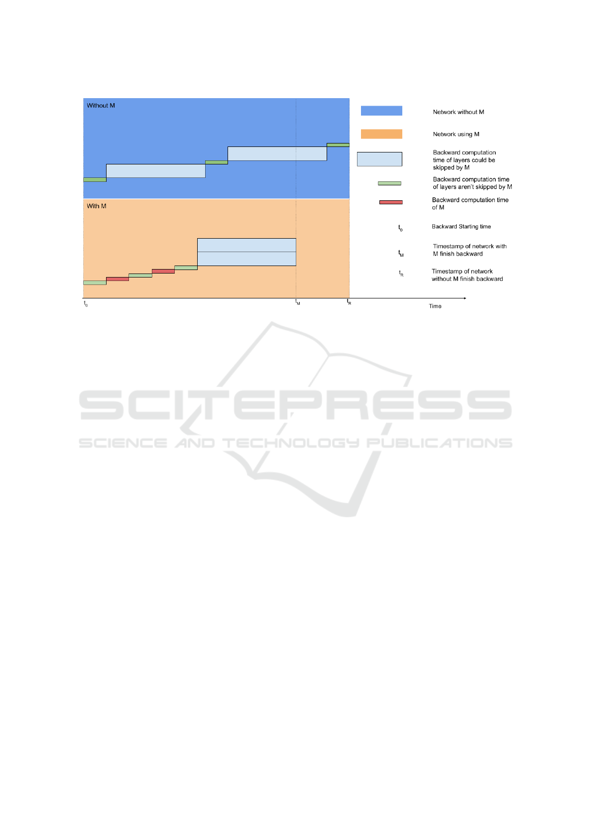
Figure 2: A comparison of backpropagation computation with and without M. Observe that the backward computation of the

layers abstracted by multiple M matrices have their gradient computation decoupled.

attuned to learning XOR logic than to other logic (Gi-

don et al., 2020).

While network modularization of this form has

yet to be explored in artiﬁcial neural networks, bi-

ological neural network modularization is well un-

derstood. There is a link between how optimization

algorithms are associated with network modulariza-

tion in the biological brain. In the biological brain,

neuronal connections are maintained and updated by

different neurotransmitters, which inﬂuences neurons

to exhibit different weight update behaviors (Amunts

et al., 2010; Huang and Reichardt, 2001). More-

over, in different brain regions, neurotransmitter types

vary (Amunts et al., 2010; Amunts and Zilles, 2015;

Huang and Reichardt, 2001; Paxinos and Mai, 2003).

Such variation results in different weight update be-

haviors forming distinct brain regions which carry out

different functions (Amunts et al., 2010), (Amunts

and Zilles, 2015; Huang and Reichardt, 2001; Paxinos

and Mai, 2003). With our M algorithm enabling usage

of different optimization algorithms, we can mimic

the existence of different neurotransmitters in differ-

ent brain regions. Therefore, training with M enables

a way toward bringing biological brain modulariza-

tion into artiﬁcial neural networks.

6 CONCLUSIONS

This work has presented a biologically-inspired learn-

ing mechanism whereby approximate gradient infor-

mation is propagated quickly through the network via

a set of abstraction matrices M

. This decouples gra-

dient computation of each set of abstracted layers.

Decoupled computation allows the weight updates

within each block of abstracted layers to be theoret-

ically executed in parallel, with potential applications

for speeding up the backward pass of large compu-

tationally expensive networks. The next logical step

in this line of research would be the utilization of ab-

straction matrices to create a depth-wise parallelized

network architecture, and to explore potential appli-

cations toward online learning and real-time network

updates.

The gradient abstraction techniques introduced in

this work have research potential that extends beyond

gradient decoupling. In biological brains, cortico-

basal ganglia pathways – mimicked in our work by

abstraction matrices – and localized logic updates are

not mutually exclusive. It is often the case that im-

precise learning signals are propagated quickly via

the cortico-basal ganglia feedback loops, then fol-

lowed by more precise updates mediated by retro-

grade synaptic connections between neurons (Sesack

and Grace, 2010; Wilson and Nicoll, 2001). Our

method for propagating abstracted gradients could be

leveraged toward a similar setup where network pa-

rameters are updated both via the abstraction matrix

and also via more traditional methods. This idea has

particular relevance in the domain of neuromorphic

computing and spiking neural networks.

ICAART 2024 - 16th International Conference on Agents and Artiﬁcial Intelligence

514

REFERENCES

Alger, B. E. (2002). Retrograde signaling in the regulation

of synaptic transmission: Focus on endocannabinoids.

Progress in Neurobiology, 68(4):247 – 286. Cited by:

486.

Amari, S. (1993). Backpropagation and stochastic gradient

descent method. Neurocomputing, 5:185–196.

Amunts, K., Lenzen, M., Friederici, A. D., Schleicher, A.,

Morosan, P., Palomero-Gallagher, N., and Zilles, K.

(2010). Broca’s region: Novel organizational princi-

ples and multiple receptor mapping. PLOS Biology,

8(9):1–16.

Amunts, K. and Zilles, K. (2015). Architectonic map-

ping of the human brain beyond brodmann. Neuron,

88(6):1086–1107.

Banerjee, S. and Lavie, A. (2005). METEOR: An automatic

metric for MT evaluation with improved correlation

with human judgments. In Proceedings of the ACL

Workshop on Intrinsic and Extrinsic Evaluation Mea-

sures for Machine Translation and/or Summarization,

pages 65–72, Ann Arbor, Michigan. Association for

Computational Linguistics.

Black, S., Gao, L., Wang, P., Leahy, C., and Biderman, S.

(2021). GPT-Neo: Large Scale Autoregressive Lan-

guage Modeling with Mesh-Tensorﬂow.

Block, H. D., Knight Jr, B., and Rosenblatt, F. (1962). Anal-

ysis of a four-layer series-coupled perceptron. ii. Re-

views of Modern Physics, 34(1):135.

Brown, T. B., Mann, B., Ryder, N., Subbiah, M., Kaplan, J.,

Dhariwal, P., Neelakantan, A., Shyam, P., Sastry, G.,

Askell, A., Agarwal, S., Herbert-Voss, A., Krueger,

G., Henighan, T., Child, R., Ramesh, A., Ziegler,

D. M., Wu, J., Winter, C., Hesse, C., Chen, M., Sigler,

E., Litwin, M., Gray, S., Chess, B., Clark, J., Berner,

C., McCandlish, S., Radford, A., Sutskever, I., and

Amodei, D. (2020). Language models are few-shot

learners.

Burke, D., Kiernan, M. C., and Bostock, H. (2001). Ex-

citability of human axons. Clinical Neurophysiology,

112(9):1575 – 1585. Cited by: 368.

Carion, N., Massa, F., Synnaeve, G., Usunier, N., Kirillov,

A., and Zagoruyko, S. (2020). End-to-end object de-

tection with transformers. In Computer Vision–ECCV

2020: 16th European Conference, Glasgow, UK, Au-

gust 23–28, 2020, Proceedings, Part I 16, pages 213–

229. Springer.

Cettolo, M., Federico, M., Bentivogli, L., Niehues, J.,

uker, S., Sudoh, K., Yoshino, K., and Federmann,

C. (2017). Overview of the IWSLT 2017 evaluation

campaign. In Proceedings of the 14th International

Conference on Spoken Language Translation, pages

2–14, Tokyo, Japan. International Workshop on Spo-

ken Language Translation.

Chen, T., Xu, B., Zhang, C., and Guestrin, C. (2016). Train-

ing deep nets with sublinear memory cost. arXiv

preprint arXiv:1604.06174.

Chen, X., Wu, Y., Wang, Z., Liu, S., and Li, J. (2021).

Developing real-time streaming transformer trans-

ducer for speech recognition on large-scale dataset.

In ICASSP 2021-2021 IEEE International Confer-

ence on Acoustics, Speech and Signal Processing

(ICASSP), pages 5904–5908. IEEE.

Cohen, G., Afshar, S., Tapson, J., and Van Schaik, A.

(2017). Emnist: Extending mnist to handwritten let-

ters. In 2017 international joint conference on neural

networks (IJCNN), pages 2921–2926. IEEE.

Deng, L. (2012). The mnist database of handwritten digit

images for machine learning research. IEEE Signal

Processing Magazine, 29(6):141–142.

Dong, L., Xu, S., and Xu, B. (2018). Speech-transformer: a

no-recurrence sequence-to-sequence model for speech

recognition. In 2018 IEEE international conference

on acoustics, speech and signal processing (ICASSP),

pages 5884–5888. IEEE.

Dosovitskiy, A., Beyer, L., Kolesnikov, A., Weissenborn,

D., Zhai, X., Unterthiner, T., Dehghani, M., Minderer,

M., Heigold, G., Gelly, S., Uszkoreit, J., and Houlsby,

N. (2021). An image is worth 16x16 words: Trans-

formers for image recognition at scale.

Elliott, D., Frank, S., Sima’an, K., and Specia, L. (2016).

Multi30k: Multilingual english-german image de-

scriptions. In Proceedings of the 5th Workshop on

Vision and Language, pages 70–74. Association for

Computational Linguistics.

Foundation, T. P. (2023). Multiprocess-

ing package - torch.multiprocessing.

https://pytorch.org/docs/stable/multiprocessing.html.

Gerdeman, G. L., Ronesi, J., and Lovinger, D. M. (2002).

Postsynaptic endocannabinoid release is critical to

long-term depression in the striatum. Nature Neuro-

science, 5(5):446 – 451. Cited by: 607.

Gidon, A., Zolnik, T. A., Fidzinski, P., Bolduan, F., Pa-

poutsi, A., Poirazi, P., Holtkamp, M., Vida, I., and

Larkum, M. E. (2020). Dendritic action potentials and

computation in human layer 2/3 cortical neurons. Sci-

ence, 367(6473):83–87.

unther, S., Ruthotto, L., Schroder, J. B., Cyr, E. C., and

Gauger, N. R. (2019). Layer-parallel training of deep

residual neural networks.

Gregor Koehler, A. A. and Markovics, P. (2020).

Mnist handwritten digit recognition in pytorch.

https://nextjournal.com/gkoehler/pytorch-mnist.

Griewank, A. and Walther, A. (2000). Algorithm 799: re-

volve: an implementation of checkpointing for the

reverse or adjoint mode of computational differenti-

ation. ACM Transactions on Mathematical Software

(TOMS), 26(1):19–45.

Gulati, A., Qin, J., Chiu, C.-C., Parmar, N., Zhang, Y., Yu,

J., Han, W., Wang, S., Zhang, Z., Wu, Y., and Pang, R.

(2020). Conformer: Convolution-augmented Trans-

former for Speech Recognition. In Proc. Interspeech

2020, pages 5036–5040.

Hardingham, N., Dachtler, J., and Fox, K. (2013). The role

of nitric oxide in pre-synaptic plasticity and home-

ostasis. Frontiers in Cellular Neuroscience, (OCT).

Cited by: 176; All Open Access, Gold Open Access,

Green Open Access.

He, K., Zhang, X., Ren, S., and Sun, J. (2015). Deep resid-

ual learning for image recognition.

Decoupling the Backward Pass Using Abstracted Gradients

515

Huang, E. and Reichardt, L. (2001). Neurotrophins: Roles

in neuronal development and function. Annual Review

of Neuroscience, 24:677 – 736. Cited by: 3394; All

Open Access, Green Open Access.

Huang, Y., Cheng, Y., Bapna, A., Firat, O., Chen, D., Chen,

M., Lee, H., Ngiam, J., Le, Q. V., Wu, Y., et al. (2019).

Gpipe: Efﬁcient training of giant neural networks us-

ing pipeline parallelism. Advances in neural informa-

tion processing systems, 32.

Klein, G., Kim, Y., Deng, Y., Senellart, J., and Rush, A. M.

(2017). Opennmt: Open-source toolkit for neural ma-

chine translation. In Proc. ACL.

Koehler, G. (2020). Mnist handwritten digit recognition in

pytorch.

Letzkus, J. J., Kampa, B. M., and Stuart, G. J. (2006).

Learning rules for spike timing-dependent plasticity

depend on dendritic synapse location. Journal of Neu-

roscience, 26(41):10420 – 10429. Cited by: 217; All

Open Access, Bronze Open Access, Green Open Ac-

cess.

Lillicrap, T. P., Cownden, D., Tweed, D. B., and Akerman,

C. J. (2016). Random synaptic feedback weights sup-

port error backpropagation for deep learning. Nature

communications, 7(1):13276.

Neftci, E. O., Augustine, C., Paul, S., and Detorakis, G.

(2017). Event-driven random back-propagation: En-

abling neuromorphic deep learning machines. Fron-

tiers in Neuroscience, 11.

Ouyang, L., Wu, J., Jiang, X., Almeida, D., Wainwright,

C. L., Mishkin, P., Zhang, C., Agarwal, S., Slama, K.,

Ray, A., Schulman, J., Hilton, J., Kelton, F., Miller,

L., Simens, M., Askell, A., Welinder, P., Christiano,

P., Leike, J., and Lowe, R. (2022). Training language

models to follow instructions with human feedback.

Papineni, K., Roukos, S., Ward, T., and Zhu, W.-J. (2002).

Bleu: a method for automatic evaluation of machine

translation. In Proceedings of the 40th Annual Meet-

ing of the Association for Computational Linguistics,

pages 311–318, Philadelphia, Pennsylvania, USA.

Association for Computational Linguistics.

Paxinos, G. and Mai, J. K. (2003). The Human Nervous

System. Cited by: 24.

Radford, A., Wu, J., Child, R., Luan, D., Amodei, D.,

Sutskever, I., et al. (2019). Language models are un-

supervised multitask learners. OpenAI blog, 1(8):9.

Rei, R., Stewart, C., Farinha, A. C., and Lavie, A. (2020).

COMET: A neural framework for MT evaluation. In

Proceedings of the 2020 Conference on Empirical

Methods in Natural Language Processing (EMNLP),

pages 2685–2702, Online. Association for Computa-

tional Linguistics.

Seger, C. A. and Miller, E. K. (2010). Category learning

in the brain. Annual Review of Neuroscience, 33:203

– 219. Cited by: 242; All Open Access, Green Open

Access.

Sesack, S. R. and Grace, A. A. (2010). Cortico-basal

ganglia reward network: Microcircuitry. Neuropsy-

chopharmacology, 35(1):27 – 47. Cited by: 732; All

Open Access, Bronze Open Access, Green Open Ac-

cess.

Song, Y., Meng, C., Liao, R., and Ermon, S. (2021). Ac-

celerating feedforward computation via parallel non-

linear equation solving.

Srivastava, R. K., Greff, K., and Schmidhuber, J. (2015).

Highway networks. arXiv preprint arXiv:1505.00387.

Stuart, G. J. and H

ausser, M. (2001). Dendritic coincidence

detection of epsps and action potentials. Nature Neu-

roscience, 4(1):63 – 71. Cited by: 279.

Vaswani, A., Shazeer, N., Parmar, N., Uszkoreit, J., Jones,

L., Gomez, A. N., Kaiser, L., and Polosukhin, I.

(2017). Attention is all you need.

Wilson, R. and Nicoll, R. (2001). Endogenous cannabi-

noids mediate retrograde signalling at hippocampal

synapses. Nature, 410(6828):588 – 592. Cited by:

1267.

Xiao, H., Rasul, K., and Vollgraf, R. (2017). Fashion-

mnist: a novel image dataset for benchmarking ma-

chine learning algorithms. CoRR, abs/1708.07747.

APPENDIX

Extended Ablation Results and

Additional Experiments

Extended Results. We present here an expanded ta-

ble demonstrating results on both derived M and M=I,

along with the additional SacreBLEU scoring metric.

This experiment seeks to answer the following

question: Is it possible that the use of the M=I ab-

straction is effective, not because M=I is a reasonable

approximation for the gradients, but because the net-

work is learning, in effect, to ignore the intervening

network layers. In other words, would it be more ef-

fective to simple train a smaller network rather than

using M=I as an abstracted gradient representation?

We address this question by comparing abstracted

models of various size with corresponding non-

abstracted models in which the layers bridged by M

have been entirely removed. If the ablated version of

each model matches the performance of the abstracted

model, then that would suggest that the abstraction is

in fact not useful for learning, and is instead simply

functioning as a mechanism to simulate a model with

fewer layers overall. Results are shown in Table 5.

Abstraction Position Experiment. Here we in-

vestigate the impact of abstraction layer positioning

on model performance. We provide an ablation study

where we vary the position of the abstraction matrix

within the transformer model. Results are shown in

Table 6.

Abstraction Size Experiment. The power of

potential parallelization increases as we deﬁne addi-

tional abstractions or increase abstraction size. As the

ICAART 2024 - 16th International Conference on Agents and Artiﬁcial Intelligence

516

results show in Table 7, abstraction on different po-

sitions perform similar to each other before ablation.

This is a positive result as the abstraction’s usefulness

is not necessarily limited by position. However, after

ablation, A3(D234) has the most amount of perfor-

mance drop. We do not yet have an conrete explana-

tion for this behavior, so we will explore it in future

works.

We observe that for each pair of corresponding

models, the ablated version performs less well than

the abstracted version, suggesting that the model is

indeed leveraging the inherent learning capacity of

the additional layers. Additionally, the performance

drop from the abstracted models is about the same as

the drop seen in the baseline model when the same

layers are removed. We therefore conclude that the

question above can be answered in the negative. The

abstraction M=I is indeed preserving useful learning

capacity in the abstracted layers. We note, however,

that the performance of the model does seem slightly

better when only one layer is abstracted rather than

three. This raises the question of how many network

layers can be effectively abstracted at one time before

network performance begins to degrade. Further re-

search is needed before this question can be answered

with conﬁdence.

Additional Biological Foundations

Our work is inspired by recent ﬁndings in neuro-

science. In both biological learning and machine

learning via artiﬁcial neural networks, an update

mechanism must exist which adjusts the synaptic

weights based on observed error in the output signal.

Traditional machine learning achieves this via back-

propagated error signals, a method which is analo-

gous to the neurobiological mechanisms of backprop-

agating action potentials (Stuart and H

ausser, 2001;

Letzkus et al., 2006) and release of retrograde neuro-

transmitters (e.g. cannabinoids and nitric oxide) (Wil-

son and Nicoll, 2001; Hardingham et al., 2013)

Our work expands upon this foundation by intro-

ducing an alternate approach to the transmission of

error gradients. Researchers have observed that, in

biological brains, neither backpropagating action po-

tentials nor retrograde neurotransmitter signals typi-

cally propagate across multiple layers due to interfer-

ence from ongoing activity and ion channel activation

refractory periods (Burke et al., 2001). Instead, bio-

logical systems seem to rely on feedback loops more

distant upstream layers are connected via feedback

loops that bypass the initial layers (Sesack and Grace,

2010). We attempt to implement a similar system via

the abstraction matrix M, which is inspired in partic-

ular by the cortico-basal ganglia network for reward

learning (Sesack and Grace, 2010).

Research on cortico-basal ganglia dopamine net-

work connectivity and behavioral implications is on-

going, and much of the circuit framework is still hy-

pothetical. However, a consistent theme is that ven-

tral tegmental area (VTA) dopamine cell bodies re-

ceive sensory input and project to the ventral striatum

(i.e. nucleus accumbens) where dopamine release oc-

curs in response to rewards and associated sensory

stimuli to encode valence and form learned associ-

ations (Sesack and Grace, 2010). When a sensory

stimuli is reinforcing, it drives dopamine release onto

output medium spiny neurons (MSNs), concomitant

to glutamate signals from cortical, thalamic, amyg-

dala and hippocampal inputs encoding additional im-

portant aspects of the stimuli (such as its emotional

value) (Seger and Miller, 2010). The dopamine sig-

nal acts as a gain modulator to facilitate or diminish

propagation of that signal through MSNs. The MSNs

then propagate the signals to their respective output

layers called the direct and indirect pathways. Im-

portantly, those two pathways also form two parallel

feedback loops that have different numbers of layers

and can thus inﬂuence future VTA dopaminergic ac-

tivity through either a short or long feedback mech-

anism (Seger and Miller, 2010; Sesack and Grace,

2010). Furthermore, local striatal synaptic activity

is still tuned by retrograde cannabinoid neurotrans-

mission (Gerdeman et al., 2002; Alger, 2002). Thus,

biological mechanisms can include backpropagating

techniques (i.e. retrograde transmission) or feedback

loops that skip layers to tune upstream activity.

The complexity of neurobiological feedback

mechanisms in biological brains are too complex to

imitate in their entirety. However, we take inspiration

from the behavior of dopamine signals in the cortico-

basal ganglia network in the creation of an abstraction

matrix M which allows error signals to bypass clus-

tered groups of layers in an artiﬁcial neural network.

Traditionally, artiﬁcial neural networks have ignored

these longer feedback loops and have typically fo-

cused only on backpropagating error signals between

proximate neurons. We believe that this oversight

fundamentally limits the opportunities for learning in

deep neural networks. The abstraction matrix M in-

troduces an alternative pathway for the propagation of

error signals, and as such may open new computation

paradigms for deep learning systems.

Decoupling the Backward Pass Using Abstracted Gradients

517

Table 5: Ablation study. B=BLEU, SB=SacreBLEU, M=METEOR, (a)=ablated model. Each tuple shows average ﬁnal

accuracy and standard deviation across ﬁve training runs.

n=6 (baseline) n=3 (baseline) n=6 (M=I) n=3 (M=I) n=6 (derived) n=3 (derived)

B (0.386, 0.008) (0.385, 0.011) (0.383, 0.008) (0.374, 0.010) (0.199, 0.033) (0.317, 0.017)

B(a) (0.374, 0.010) (0.380, 0.006) (0.374, 0.007) (0.372, 0.006) (0.153, 0.038) (0.299, 0.009)

SB (0.386, 0.008) (0.385, 0.011) (0.383, 0.008) (0.374, 0.010) (0.199, 0.033) (0.317, 0.017)

SB(a) (0.374, 0.007) (0.380, 0.006) (0.374, 0.007) (0.372, 0.006) (0.153, 0.038) (0.299, 0.009)

M (0.708, 0.006) (0.709, 0.007) (0.705, 0.004) (0.702, 0.007) (0.477, 0.042) (0.623, 0.016)

M(a) (0.698, 0.006) (0.704, 0.004) (0.696, 0.007) (0.697, 0.007) (0.407, 0.058) (0.603, 0.011)

Table 6: Performances of different abstraction sizes on Multi30k dataset over 10 trials. Models are transformer models with

6 encoder layers and 6 decoder layers. Abstraction method is M = I. A3(E345) means abstract 3 consecutive layers with

a single M, from 3rd to 5th encoder layers. E and D means the encoder and decoder layers respectively. And (a) means

performances measured after ablated abstracted layers.

A3(E234) A3(E345) A3(D234) A3(D345)

(acc, stddev) (acc, stddev) (acc, stddev) (acc, stddev)

BLEU (0.368, 0.010) (0.371, 0.008) (0.362, 0.007) (0.362, 0.010)

BLEU(a) (0.332, 0.006) (0.353, 0.011) (0.307, 0.010) (0.334, 0.011)

COMET (0.759, 0.004) (0.759, 0.005) (0.751, 0.004) (0.753, 0.005)

COMET(a) (0.734, 0.005) (0.749, 0.006) (0.679, 0.017) (0.715, 0.008)

METEOR (0.692, 0.007) (0.690, 0.006) (0.679, 0.007) (0.683, 0.007)

METEOR(a) (0.642, 0.009) (0.671, 0.009) (0.614, 0.014) (0.644, 0.009)

Table 7: Performances of different abstraction sizes on Multi30k dataset over 10 trials. Models above are transformer models

with 6 encoder layers and 6 decoder layers. Abstraction method in this experiment is M = I. A6(L3-5) means abstracted 6

layers in total, with two blocks of 3 consecutive layers, from 3rd to 5th layers in both the encoders and decoders.

A4(L4-5) A6(L3-5) A8(L2-5)

(acc, stddev) (acc, stddev) (acc, stddev)

BLEU (0.362, 0.010) (0.359, 0.008) (0.360, 0.011)

COMET (0.754, 0.006) (0.750, 0.005) (0.746, 0.007)

METEOR (0.684, 0.009) (0.678, 0.008) (0.678, 0.008)

ICAART 2024 - 16th International Conference on Agents and Artiﬁcial Intelligence

518