Efﬁcient Parameter Mining and Freezing for Continual Object Detection

Angelo G. Menezes

1 a

, Augusto J. Peterlevitz

2 b

, Mateus A. Chinelatto

2 c

and Andr

e C. P. L. F. de Carvalho

1 d

Institute of Mathematics and Computer Sciences, University of S

ao Paulo, S

ao Carlos, Brazil

Computer Vision Department, Eldorado Research Institute, Campinas, Brazil

Keywords:

Object Detection, Continual Learning, Continual Object Detection, Replay, Parameter Mining.

Abstract:

Continual Object Detection is essential for enabling intelligent agents to interact proactively with humans in

real-world settings. While parameter-isolation strategies have been extensively explored in the context of con-

tinual learning for classiﬁcation, they have yet to be fully harnessed for incremental object detection scenarios.

Drawing inspiration from prior research that focused on mining individual neuron responses and integrating

insights from recent developments in neural pruning, we proposed efﬁcient ways to identify which layers are

the most important for a network to maintain the performance of a detector across sequential updates. The

presented ﬁndings highlight the substantial advantages of layer-level parameter isolation in facilitating incre-

mental learning within object detection models, offering promising avenues for future research and application

in real-world scenarios.

1 INTRODUCTION

In the era of pervasive computing, computer vision

has emerged as a central ﬁeld of study with an ar-

ray of applications across various domains, includ-

ing healthcare, autonomous vehicles, robotics, and

security systems (Wu et al., 2020). For real-world

computer vision applications, continual learning, or

the ability to learn from a continuous stream of data

and adapt to new tasks without forgetting previous

ones, plays a vital role. It enables models to adapt

to ever-changing environments and learn from a non-

stationary distribution of data, mirroring human-like

learning (Shaheen et al., 2021). This form of learn-

ing becomes increasingly signiﬁcant as the demand

grows for models that can evolve and improve over

time without the need to store all the data and be

trained from scratch.

Within computer vision, object detection is a fun-

damental task aiming at identifying and locating ob-

jects of interest within an image. Historically, two-

stage detectors, comprising a region proposal network

followed by a classiﬁcation stage, were the norm,

but they often suffer from increased complexity and

https://orcid.org/0000-0002-7995-096X

https://orcid.org/0000-0003-0575-9633

https://orcid.org/0000-0002-6933-213X

https://orcid.org/0000-0002-4765-6459

slower run-time (Zou et al., 2019). The emergence of

one-stage detectors, which combine these stages into

a uniﬁed framework, has allowed for more efﬁcient

and often more accurate detection (Tian et al., 2020;

Lin et al., 2017). In this context, incremental learn-

ing strategies for object detection can further comple-

ment one-stage detectors by facilitating the continu-

ous adaptation of the model to new tasks or classes,

making it highly suitable for real-world applications

where the object landscape may change over time (Li

et al., 2019; ul Haq et al., 2021).

Recent works have concluded that catastrophic

forgetting is enlarged when the magnitude of the cal-

culated gradients becomes higher for accommodat-

ing the new knowledge (Mirzadeh et al., 2021; Had-

sell et al., 2020). Since the new parameter values

may deviate from the optimum place that was used

to obtain the previous performance, the overall mAP

metrics can decline. Traditionally in continual learn-

ing (CL) for classiﬁcation, researchers have proposed

to tackle this problem directly by applying regular-

ization schemes, often preventing important neurons

from updating or artiﬁcially aligning the gradients for

each task. Such techniques have shown fair results

at the cost of being computationally expensive since

network parameters are mostly adjusted individually

(Kirkpatrick et al., 2017; Chaudhry et al., 2018).

To account for the changes and keep the detector

466

Menezes, A., Peterlevitz, A., Chinelatto, M. and de Carvalho, A.

Efﬁcient Parameter Mining and Freezing for Continual Object Detection.

DOI: 10.5220/0012362300003660

Paper published under CC license (CC BY-NC-ND 4.0)

In Proceedings of the 19th International Joint Conference on Computer Vision, Imaging and Computer Graphics Theory and Applications (VISIGRAPP 2024) - Volume 2: VISAPP, pages

466-474

ISBN: 978-989-758-679-8; ISSN: 2184-4321

aligned with their previous performances, most works

in continual object detection (COD) mitigate forget-

ting with regularization schemes based on complex

knowledge distillation strategies and their combina-

tion with replay or the use of external data (Menezes

et al., 2023). However, we argue that the results pre-

sented by the solo work of Li et al. (2018) indicate

that there is room to investigate further parameter-

isolation schemes for COD. For these strategies, the

most important neurons for a task are identiﬁed, and

their changes are softened across learning updates to

protect the knowledge from previous tasks.

In this paper, we propose a thorough investigation

of efﬁcient ways to identify and penalize the change

in weights for sequential updates of an object detec-

tor using insights from the neural pruning literature.

We show that by intelligently freezing full signiﬁcant

layers of neurons, one might be able to alleviate catas-

trophic forgetting and foster a more efﬁcient and ro-

bust detector.

2 RELATED WORK

The concept of using priors to identify the importance

of the weights and protect them from updating is not

new in CL. Kirkpatrick et al. (2017) proposed a reg-

ularization term on the loss function that penalizes

the update of important parameters. These parame-

ters are estimated by calculating the Fish information

matrix for each weight, which considers the distance

between the current weight values and the optimal

weights obtained when optimizing for the previous

task. (Zenke et al., 2017) similarly regularized the

new learning experiences but kept an online estimate

of the importance of each parameter. Both strategies

compute the change needed for each individual pa-

rameter, which can be computationally challenging

for large-scale detectors.

Also, on the verge of regularization, Li and Hoiem

(2017) saved a copy of the model after training for

each task and, when learning a new task, applied

knowledge distillation on the outputs to make sure

the current model could keep responses close to the

ones produced in previous tasks. Such a strategy

was adapted for COD in the work of Shmelkov et al.

(2017), which proposed to distill knowledge from

the ﬁnal logits and bounding box coordinates. Li

et al. (2019) went further and introduced an additional

distillation on intermediate features for the network.

Both strategies have been used in several subsequent

works in COD as strong baselines for performance

comparison.

In CL for classiﬁcation, Mallya and Lazebnik

(2018) conceptualized PackNet, which used concepts

of the neural pruning literature for applying an iter-

ative parameter isolation strategy. It ﬁrst trained a

model for a task and pruned the lowest magnitude pa-

rameters, as they were seen as the least contributors

to the model’s performance. Then, the left parame-

ters were ﬁne-tuned on the initial task data and kept

frozen across new learning updates. Such a strategy

is usually able to mitigate forgetting, through the cost

of lower plasticity when learning new tasks. Simi-

larly, Li et al. (2018) proposed a strategy, here denoted

as MMN, to “mine” important neurons for the incre-

mental learning of object detectors. Their method in-

volved ranking the weights of each layer in the orig-

inal model and retaining (i.e., ﬁxing the value of) the

Top-K neurons to preserve the discriminative infor-

mation of the original classes, leaving the other pa-

rameters free to be updated but not zeroed as initially

proposed by PackNet. The importance of each neu-

ron is estimated by sorting them based on the abso-

lute value of their weight. The authors evaluated this

strategy with variations of the percentage of neurons

to be frozen and found that a 75% value was ideal for

a stability-plasticity balance within the model. Al-

though simple, the ﬁnal described performance was

on par with the state-of-the-art of the time (Shmelkov

et al., 2017).

The above parameter-isolation strategies for CL

consider that the most important individual neurons

will present the highest absolute weight values and

must be kept unchanged when learning new tasks.

This is a traditional network pruning concept and is

commonly treated as a strong baseline (LeCun et al.,

1989; Li et al., 2016). However, Neural Network

Pruning strategies have evolved to also consider the

ﬁlter and layer-wise dynamics. For that, the impor-

tance of a ﬁlter or the whole layer can be obtained

by analyzing the feature maps after the forward pass

of a subset of the whole dataset. Then, they can be

ranked and pruned based on criteria such as proxim-

ity to zero, variation inter samples, or information en-

tropy (Liu and Wu, 2019; Luo and Wu, 2017; Wang

et al., 2021). Even so, the available network capac-

ity will be dependent on the number of involved tasks

since important parameters are not allowed to change.

3 METHODOLOGY

Based on the recent neural pruning literature, we ex-

plore four different ways to identify important param-

eters to be kept intact across sequential updates. The

following criteria are used to determine the impor-

tance of each network layer after forwarding a subset

Efﬁcient Parameter Mining and Freezing for Continual Object Detection

467

of images from the task data and analyzing the gener-

ated feature maps:

• Highest Mean of Activation Values. Rank and

select the layers with ﬁlters that produced the

highest mean of activations.

I(layer

) =

∑

k=1

F(x

) (1)

• Highest Median of Activation Values. An alter-

native that considers the highest median of activa-

tions instead of the mean.

I(layer

) = Med(F(x

)) (2)

• Highest Variance. For this criterion, we consider

that ﬁlters with higher standard deviation in the

generated feature maps across diverse samples are

more important and their layer should be kept un-

changed.

I(layer

) =

∑

k=1

(F(x

) − µ)

(3)

• Highest Information Entropy. Rank and select

the layers based on the highest information en-

tropy on their feature maps.

I(layer

) = −

∑

k=1

P(F(x

))log

P(F(x

)) (4)

where N is the number of images in the subset; F(x

)

is the ﬂattened feature map; Med is the median of the

feature map activations; µ is mean of the feature map

activations; P is the probability distribution of a fea-

ture map.

Additionally, in a separate investigation, we ex-

plore whether relaxing the ﬁxed weight constraint

proposed by MMN can allow the model to be more

plastic while keeping decent performance on previ-

ous tasks. For that, we propose to simply adjust the

changes to the mined task-speciﬁc parameters during

the training step by multiplying the gradients calcu-

lated in the incremental step by a penalty value. By al-

lowing them to adjust the important weights in a min-

imal way (i.e., with a penalty of 1% or 10%) across

tasks, we hypothesize that the model will be able to

circumvent capacity constraints and be more plastic.

For the proposed layer-mining criteria, we also

check which percentage (i.e., 25, 50, 75, 90) of frozen

layers would give the best results. Figure 1 describes

the proposed experimental pipeline.

3.1 Evaluation Benchmarks

Two different incremental learning scenarios were

used to check the performance of the proposed meth-

ods.

Incremental Pascal VOC. We opted to use the incre-

mental version of the well-known Pascal VOC dataset

following the 2-step learning protocol used by the ma-

jority of works in the area (Menezes et al., 2023). We

investigated the scenarios in which the model needs

to learn either the last class or the last 10 classes at

once, as described in Figure 2.

TAESA Transmission Towers Dataset. The detec-

tion of transmission towers and their components us-

ing aerial footage is an essential step for perform-

ing inspections on their structures. These inspections

are often performed by onsite specialists to catego-

rize the health aspect of each component. The advan-

tage of automating such tasks by the use of drones has

been largely approached in this industry setting and is

known to have a positive impact on standardization

of the acquisition process and reducing the number of

accidents in locu. However, there is a lack of success-

ful reports of general applications in this ﬁeld since

it inherently involves several challenges related to ac-

quiring training data, having to deal with large do-

main discrepancies (since energy transmission towers

can be located anywhere in a country), and the neces-

sity to update the model every time a new accessory

or tower needs to be mapped.

To aid in the proposal of solutions for some of

the listed issues, we introduce the TAESA Transmis-

sion Towers Dataset. It consists of aerial images from

several drone inspections performed on energy trans-

mission sites maintained by the TAESA company in

Brazil. The full dataset has records from different

transmission sites from four cities with different soil

and vegetation conditions. In this way, the incremen-

tal benchmark was organized into four different learn-

ing tasks, each representing data from a speciﬁc trans-

mission site, as illustrated by Figure 3.

Each task can have new classes that were not

introduced before and new visuals for a previously

introduced object, making it a challenging “data-

incremental” benchmark. In addition, different from

most artiﬁcial benchmarks, images were annotated by

several people using a reference sheet of the possible

classes that could be present. For that, the possibility

of missing annotations and label conﬂict in posterior

tasks was reduced. A summary of the dataset with re-

spect to the number of images and objects, with their

description, for each task can be seen in Tables 2 and

3.2 Implementation Details

We opted to explore the RetinaNet one-stage detector

using a frozen ResNet50 with an unfrozen FPN back-

bone. The selected freezing criteria is therefore only

VISAPP 2024 - 19th International Conference on Computer Vision Theory and Applications

468

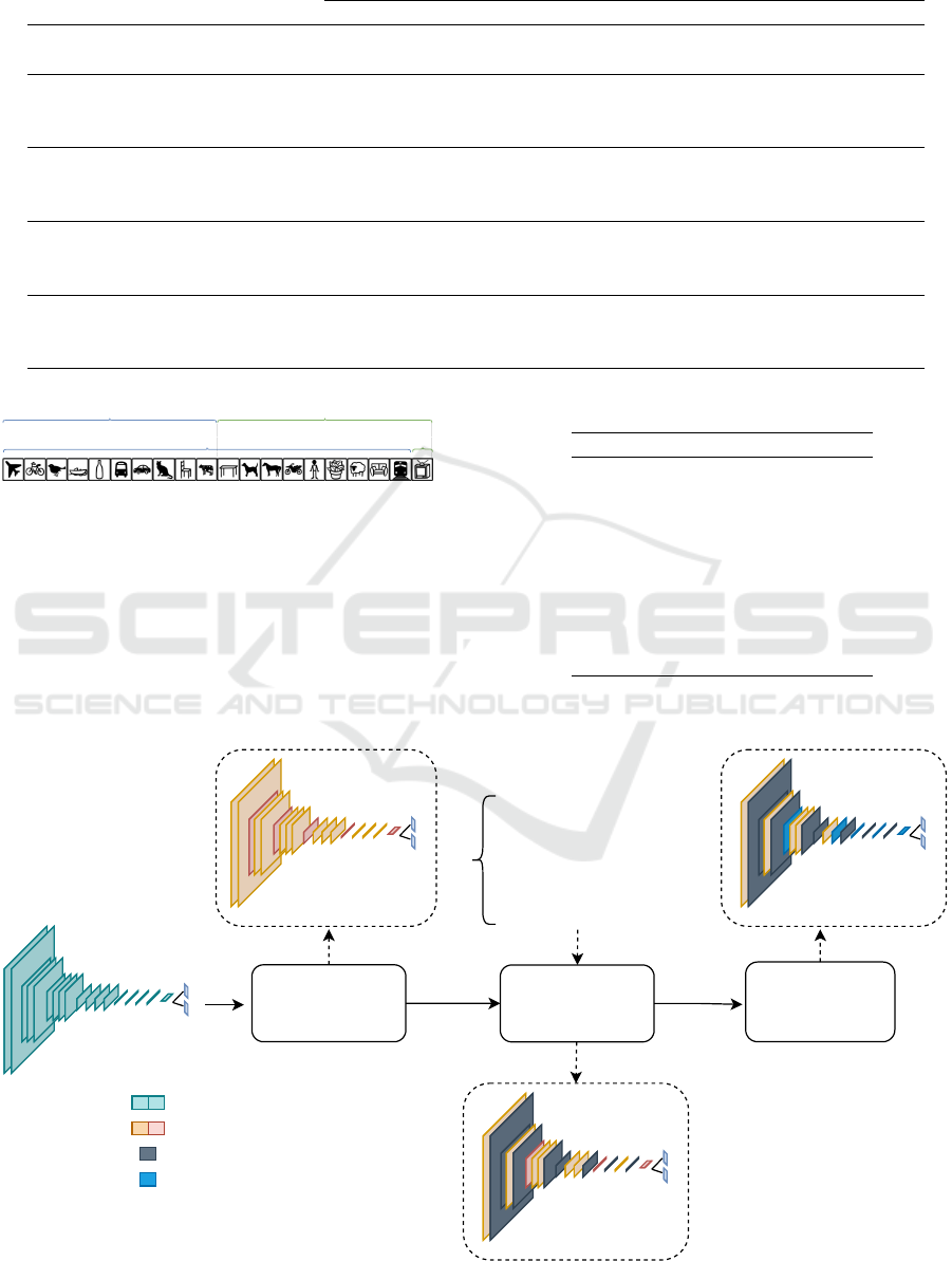
Table 1: TAESA Dataset Summary.

◦

of Boxes per label

Scenario Set

◦

Images

0 1 2 3 4 5 6 7 8

Total

Boxes

Task 1

Training 526 690 2228 482 119 381 528 - - - 4428

Validation 67 78 245 55 16 29 49 - - - 472

Testing 69 91 252 49 10 42 60 - - - 504

Task 2

Training 431 86 950 260 4 - - 20 429 8 1757

Validation 55 14 120 32 - - - 2 55 - 223

Testing 55 2 120 29 1 - - 3 55 - 210

Task 3

Training 308 5 726 269 39 - - 303 - 4 1346

Validation 39 3 92 31 5 - - 36 - - 167

Testing 39 1 89 33 6 - - 38 - - 167

Task 4

Training 227 5 1242 357 - 770 83 - - 234 2691

Validation 28 2 165 50 - 98 12 - - 29 356

Testing 29 - 177 52 - 112 11 - - 29 381

VOC Base Classes 1-10

VOC Base Classes 1-19

VOC Incremental Classes 11-20

VOC Incremental

Class 20

Figure 2: Incremental PASCAL VOC Benchmark Evalu-

ated Scenarios.

applied to the neck (i.e., FPN) and head of the model.

The training settings are similar to the ones proposed

by Shmelkov et al. (2017). For both benchmarks, the

model was trained with SGD for 40k steps with an LR

of 0.01 for learning the ﬁrst task. For the incremental

tasks, in the Pascal VOC Benchmark, the model was

trained with an LR of 0.001 for more 40k steps when

presented with data from several classes and for 5k

Table 2: ID for each class in the TAESA dataset.

Class Label Description

0 Classic Tower

1 Insulator

2 Yoke Plate

3 Clamper

4 Ball Link

5 Anchoring Clamp

6 Guyed Tower

7 Support Tower

8 Anchor Tower

Traning for

task tn

Mining important

parameters

Class

logits

BBox

Predictions

Traning for

task tn+1

Weights not tunned

Weights tunned for task

Frozen weights

Weights tunned for task

n+1

Freezing weights

- Max absolute weight value

Freezing layers

- Max mean activation value

- Max activation variation

- Max activation entropy

Figure 1: Mining important parameters for efﬁcient incremental updates.

Efﬁcient Parameter Mining and Freezing for Continual Object Detection

469

Figure 3: Sample of images of each task for the TAESA

Transmission Towers Dataset.

steps when only data from the last class was used. For

the incremental tasks with the TAESA benchmark, the

model was trained with an LR of 0.001 for 5k steps for

each new task. The code for training the network was

written in Python and used the MMDetection toolbox

for orchestrating the detection benchmark and evalua-

tion procedure (Chen et al., 2019). The main followed

steps are depicted below in Algorithm 1.

As for the baselines, for the Incremental Pascal

VOC benchmark, we considered the results reported

on the work of Li et al. (2019) for the ILOD and

RILOD strategies which also made use of the Reti-

naNet with ResNet50 as the backbone in a similar

training setting. For the TAESA benchmark, we pro-

pose the comparison against Experience Replay us-

ing a task-balanced random reservoir buffer. We also

compare the results in both benchmarks against our

implementation of the MMN strategy from Li et al.

(2018) as well as the upper bound when all data is

available for training the model. To account for the

randomness associated with neural networks, we re-

port the performance of each strategy after the aver-

aging of three runs with different seeds.

3.3 Evaluation Metrics

For checking the performance in the Incremental Pas-

cal VOC benchmark, we use the average mAP[.5] and

Ω for comparisons against the upper bound (i.e., join-

training) as usually reported by other works. To better

evaluate the potential of each strategy regarding the

model‘s ability to retain and acquire new knowledge,

we also apply the metrics proposed by Menezes et al.

(2023) known as the rate of stability (RSD) and plas-

ticity (RPD) deﬁcits, described in Equations 5 and 6.

Algorithm 1: Incremental training with parameter mining

and freezing for COD.

1: M: Model to be trained

2: Tasks: List of learning experiences

3: S: Type of mining strategy

4: L: Percentage L of frozen layers or parameters

5: P: Percentage of gradient penalty

6: C: Criteria for freezing the layers

7: N: Percentage of samples from Task

to be used

for calculating freezing metrics

8: i ← 0

9: for i in range(length(Tasks)) do:

10: Train model M with data from Task

11: if S = gradient mining then

12: Dump previous gradient hooks

13: Attach a hook with the gradient penalty P

to the selected percentage L of parameters

14: end if

15: if S = layer f reezing then

16: Reset requires gr ad of the parameters in

each layer

17: Freeze a percentage L of the layers given

the chosen criteria C using statistics from the fea-

ture maps obtained after forwarding the N se-

lected samples

18: end if

19: Fine-tune in Task

for 1k steps to regularize

parameters for the next learning experience

20: i ← i + 1

21: end for

22: return M

RSD =

old classes

∑

i=1

mAP

joint,i

− mAP

inc,i

mAP

joint,i

∗ 100 (5)

RPD =

new classes

∑

i=N

old classes

mAP

joint,i

− mAP

inc,i

mAP

joint,i

∗ 100 (6)

Especially for the TAESA benchmark, the per-

formance is measured by the ﬁnal mAP, with differ-

ent thresholds, and mAP[.50] after learning all tasks,

as well as with their upper-bound ratios Ω

mAP

and

Ω

mAP[.50]

. Additionally, since the benchmark involves

the introduction of a sequence of tasks, we have mod-

iﬁed the existing RSD and RPD metrics to consider

individual tasks instead of classes. In this evalua-

tion scenario, RSD measures the performance deﬁcit

against the upper bound mAP in all tasks up to the

last one, while RPD evaluates the performance deﬁcit

against the last learned task.

VISAPP 2024 - 19th International Conference on Computer Vision Theory and Applications

470

4 RESULTS

4.1 Pascal VOC 1-19 + 20

Table 3 describes the performance of each strategy

for the 19 + 1 scenario. For this scenario, we no-

ticed that the ﬁnal mAP and Ω

all

would heavily ben-

eﬁt models that were more stable than plastic since

there was a clear imbalance in the number of repre-

sented classes (i.e., 19 → 1) for the incremental step.

With that in mind, we analyzed the results that bet-

ter balanced the decrease in RSD and RPD since,

by splitting the deﬁcits in performance, it is clearer

to understand the ability to forget and adapt in each

model. By comparing the results of the application

of gradient penalty with respect to freezing the neu-

rons with the highest magnitude (i.e., MMN in Ta-

ble 3), we see that allowing the extra plasticity did

not produce broad effects in performance. However,

when 90% of the weights were mined, the extra ad-

justments introduced by using 1% of the calculated

gradients allowed the model to beat MMN. Regard-

ing the results of layer-mining, freezing based on in-

formation entropy presented a better balance in RS D

and RPD, even against more established techniques

such as ILOD and RILOD. For most of the results, in-

creasing the percentage of frozen layers gave a lower

deﬁcit in stability with the caveat of increasing the dif-

ference in mAP against the upper bound for the new

learned class.

Overall, leaving a lower percentage of parameters

frozen across updates for the methods that worked on

individual neurons made their networks more adapt-

able. Yet, this hyperparameter for the layer-freezing

methods did not greatly affect the learning of the new

class but had a signiﬁcant impact on the detection of

classes that had been learned previously.

4.2 Pascal VOC 1-10 + 11-20

Table 4 reports the results for the 10 + 10 alterna-

tive. For this scenario, the ﬁnal mAP and Ω

all

be-

came more relevant as there was an equal representa-

tion of classes for their calculations. Results for ap-

plying a penalty to the gradient of selected neurons

showed a slightly superior performance compared to

completely freezing them. This was especially true in

all scenarios where a 10% penalty was applied. For

this benchmark, freezing 25% of the layers based on

information entropy yielded the best results, followed

by using the median of the activations to the same

percentage of frozen layers. However, the ﬁnal mAP

and Ω

all

indicate that these simply arranged strate-

gies might have a difﬁcult time competing against tra-

ditional methods when processing a benchmark with

more complexities. Nonetheless, they can still serve

as a quick and strong baseline when compared to ﬁne-

tuning and MMN due to ease of implementation.

Overall for the 10 + 10 scenario, all evaluated

strategies produced comparable ﬁnal in terms of mAP

and Ω

all

. Nevertheless, the best outcomes were ob-

served when freezing or penalizing 50% or less of the

parameters. Since most detectors based on deep neu-

ral networks are overparameterized and not optimized

directly for sparse connections, freezing more than

50% of available parameters or layers might affect

highly the network capacity for learning new objects.

We believe this to be true mainly for learning new

tasks with imbalanced category sets and objects that

do not present visual similarities with the ones previ-

ously learned. The Incremental Pascal VOC bench-

mark presents not only an imbalanced occurrence of

each category but also a considerable semantic differ-

ence for the labels of the two tasks, with the ﬁrst hav-

ing more instances from outdoor environments and

the second focusing on instances from indoor scenes.

This can be further investigated by exploring task-

relatedness as a way to deﬁne the parameters that de-

termine how layer-freezing should take place between

updates.

Interestingly, as also shown in the ﬁnal evaluation

remarks of the PackNet strategy for classiﬁcation, the

ﬁnal performance of the incremental model can be

weakened since it only uses a fraction of the entire pa-

rameter set to learn new tasks (Delange et al., 2021).

However, this tradeoff is necessary to ensure stable

performance in the tasks that were initially learned.

Considering the necessity for quick adaptation in con-

strained environments, having a hyperparameter to

adjust the plasticity of the model can be used as a

feature to preserve the performance in previous sce-

narios and slightly adjust the network to the new cir-

cumstances. This feature can be especially beneﬁcial

when new updates with mixed data (i.e., old and new

samples) are expected in the future.

4.3 TAESA Benchmark

Table 5 summarizes the results on the proposed

benchmark with the green color highlighting met-

rics related to mAP and blue for mAP

[.50]

. As the

benchmark involves class-incremental and domain-

incremental aspects, we noticed that when there is lit-

tle drift in the appearance of previously known objects

that show up in the new task images, these instances

reinforce the “old knowledge” and can be considered

as a small case of replay. This can be checked by the

fact that the forgetting in the ﬁne-tuning approach is

Efﬁcient Parameter Mining and Freezing for Continual Object Detection

471

Table 3: Results when learning the last class (TV monitor).

19 + 1 aero cycle bird boat bottle bus car cat chair cow table dog horse bike person plant sheep sofa train tv mAP Ω

all

↑ RSD (%)↓ RPD (%) ↓

Upper-bound 73.5 80.6 77.4 61.2 62.2 79.9 83.4 86.7 47.6 78 68.1 85.1 83.7 82.8 79.1 42.5 75.7 64.9 79 76.2 73.4 - - -

First 19 77 83.5 77.7 65.1 63 78.1 83.6 88.5 55.2 79.7 71.3 85.8 85.2 83 80.2 44.1 75.2 69.7 81.4 0 71.4 - - -

New 1 48 61.2 27.6 18.1 8.1 58.7 53.4 17.1 0 45.9 18.2 31.9 59.9 62.2 9.1 3.4 42.9 0 50.3 63.8 34.0 - - -

ILOD 61.9 78.5 62.5 39.2 60.9 53.2 79.3 84.5 52.3 52.6 62.8 71.5 51.8 61.5 76.8 43.8 43.8 69.7 52.9 44.6 60.2 0.81 18.01 45.66

RILOD 69.7 78.3 70.2 46.4 59.5 69.3 79.7 79.9 52.7 69.8 57.4 75.8 69.1 69.8 76.4 43.2 68.5 70.9 53.7 40.4 65.0 0.87 10.90 51.28

MMN

25 71.8 78.8 66.5 48.5 48.6 73.4 78.8 77.1 9.1 76.5 52.3 74.7 82.4 76.3 62.3 21.5 65.9 20.9 68.2 45.6 60.0 0.82 17.06 41.70

50 73.4 79 71.5 51 53.4 73.4 81.6 78.5 13.9 73.5 54.5 76.7 83.2 79.1 64 27.7 66.8 36.3 69.4 43 62.5 0.85 13.23 45.24

75 74.8 79.3 72.9 54.9 54 73.9 82 85 25.4 77.2 60 81.8 83.5 80.2 70.1 35.9 68 49.7 67.8 39.3 65.8 0.90 8.25 50.29

90 76.5 82.4 74.4 58.4 57.9 74.2 82.3 86.7 35.7 77.6 65.1 83.7 83.8 82.2 72.5 37 73.2 58.5 71.5 33.7 68.4 0.93 4.15 57.92

Gradient

penalty

of 1%

25 71.9 78.8 66.5 48.6 48.5 73.4 78.8 77.1 9.1 76.5 52.3 74.6 82.4 76.3 62.3 21.5 65.9 20.7 68

45.5 59.9 0.82 17.08 41.84

50 73.3 79 71.4 51 53.3 73.4 81.6 78.4 13.8 73.5 54.4 76.7 83.2 79 64 27.4 66.8 34.7 69.3 43 62.4 0.85 13.43 45.24

75 75 79.3 72.9 54.9 54 73.8 82 84.9 25.3 77.2 59.8 81.8 83.5 80.1 70.1 35.8 67.9 49.3 67.8 39.4 65.7 0.90 8.32 50.15

90 76 82.1 74.4 57.3 57.3 74.1 82.1 85.9 34 77.4 63.4 82.9 83.4 82 72.1 37.1 72.4 57.1 70.5 34.3 67.8 0.92 5.01 57.10

Gradient

penalty

of 10%

25 71.8 78.6 66.5 48 48.5 73.4 78.8 77.1 9.1 76.5 52.2 74.1 82.4 76.2 62.2 21 65.6 19.9 68.2 45.4 59.8 0.81 17.31 41.97

50 73.1 78.8 71.3 49.6 53.3 74.5 81.5 78.3 11.4 73.4 54 76.4 82.8 76.8 63.8 27 66.4 33.4 68.6 43.8 61.9 0.84 14.13 44.15

75 73.9 79.2 72.9 53.5 54.2 73.4 81.8 79.6 22 76.9 58.4 81.6 83.3 79.8 69.3 33.6 67.4 47.2 67.4 39.4 64.7 0.88 9.75 50.15

90 76.2 81.8 73.6 55.9 57 73.2 81.2 84.6 30.3 76.9 60.7 82.4 83.6 81.1 71.1 36.3 68.3 56 67 37.2 66.7 0.91 6.76 53.15

Freezing

based on

mean

25 75.1 78.8 71.6 57.3 54.3 75.3 81.1 78.6 27.5 77 60.4 80.8 82.5 79.6 70.5 32.5 72.3 57.3 74.1 31.3 65.9 0.90 7.52 61.19

50 75.3 78.6 72 57.7 53.8 74.7 81 79 27 74.7 62.5 77.8 82.7 77.5 70.5 33.1 72 56.5 73.1 32.4 65.6 0.89 8.03 59.69

75 76 79.5 73.2 58 57 75.8 81.6 84.4 27.3 77.3 64.8 82.1 82.7 80.4 71.5 36 72.7 57.4 74.8 25.2 66.9 0.91 5.66 69.50

90 76.2 81.3 71.9 60.8 49.9 75.7 82.8 86.2 24.8 76.5 69.4 82 82.9 80.9 68.5 26.2 71.9 60.3 79.4 41.7 67.5 0.92 6.01 47.02

Freezing

based on

median

25 75.1 78.7 71.7 57.3 54.4 74.8 81.2 78.7 27.4 76.9 60.1 80.8 82.5 79.3 70.6 32.3 72.5 57.3 73.6 31.3 65.8 0.90 7.62 61.19

50 75.3 78.8 72.3 57.7 56.7 74 81.6 79.4 26.5 76.9 63.1 81.8 82.6 78.9 70.8 34.7 72.8 56.2 72.9 24.4 65.9 0.90 7.06 70.59

75 78 79.6 73.2 57.1 55.7 76.1 82.6 86.1 38.3 77.2 65.8 83.1 82.4 80.5 73.7 38.5 71.6 60.5 75.4 31.2 68.3 0.93 4.02 61.32

90 77.4 82.1 72.7 61.3 50.3 77.2 82.9 85.8 28.8 76.4 69.5 82 82.8 81.2 68.5 27.5 71.7 60.4 79.1 39.6 67.9 0.92 5.29 49.88

Freezing

based on

std

25 75.1 78.9 71.6 57.3 54.3 75.3 81.1 78.6 27.5 77 60.4 80.8 82.5 77.4 70.5 32.4 72.3 57.3 74 31.5 65.8 0.90 7.68 60.92

50 75.1 78.9 71.6 57.2 54.3 75.3 81.1 78.7 27.5 77 60.4 80.7 82.5 77.4 70.5 32.3 72.3 57.3 74 31.4 65.8 0.90 7.70 61.05

75 75.7 79.1 72.9 57.1 56.4 75.2 81.4 79.3 25.2 77.4 61.5 81.6 82 79.5 70.6 33.7 72.9 56.1 74.5 27.9 66.0 0.90 7.12 65.82

90 77.6 79.9 73.5 57.3 56.6 77.7 82.8 86.2 38.2 77.1 65.9 82.8 82.5 80.2 73.7 39 72.4 61.5 76 31.5 68.6 0.94 3.62 60.92

Freezing

based on

entropy

25 75.5 79.4 72.7 56.2 57.2 74.8 81.9 84.7 28.9 77.9 62 81.4 83.1 81.1 71.6 35.3 68.4 54.7 69 40.7 66.8 0.91 6.86 48.38

50 76.8 81.6 72.5 57 52.2 74.7 83.2 78.3 22.2 73.8 63.7 78.1 81.3 80 70.7 25.3 71 45.4 74.4 57 66.0 0.90 9.27 26.17

75 76.9 81.8 71.9 61.4 50.4 76 82.7 86 29.5 76 69.6 82.3 82.9 80.7 68.6 26.7 72.1 60.9 79.6 40.5 67.8 0.92 5.41 48.65

90 77.4 81.9 72.3 61.4 50.2 76.3 82.9 85.7 30 76 69.6 82.2 82.5 81.2 68.5 27.4 72 60.7 79.4 38.2 67.8 0.92 5.29 51.79

Table 4: Results when learning the last 10 classes.

10 + 10 aero cycle bird boat bottle bus car cat chair cow table dog horse bike person plant sheep sofa train tv mAP Ω

all

↑ RSD (%) ↓ RPD (%) ↓

Upper-bound 73.5 80.6 77.4 61.2 62.2 79.9 83.4 86.7 47.6 78 68.1 85.1 83.7 82.8 79.1 42.5 75.7 64.9 79 76.2 73.4 - - -

First 10 79.2 85.6 76.5 66.7 65.9 78.9 85.2 86.6 60.2 84.7 0 0 0 0 0 0 0 0 0 0 38.5 - - -

New 10 0 0 0 0 0 0 0 0 0 0 74.6 85.7 86.1 79.9 79.8 43.9 76.3 68.5 80.5 76.3 37.6 - - -

ILOD 67.1 64.1 45.7 40.9 52.2 66.5 83.4 75.3 46.4 59.4 64.1 74.8 77.1 67.1 63.3 32.7 61.3 56.8 73.7 67.3 62.0 0.84 17.65 13.48

RILOD 71.7 81.7 66.9 49.6 58 65.9 84.7 76.8 50.1 69.4 67 72.8 77.3 73.8 74.9 39.9 68.5 61.5 75.5 72.4 67.9 0.93 7.59 7.29

MMN

25 59.2 37.4 38.7 33.3 17.2 46.3 52.9 57.5 5.9 45.7 62.9 73.6 76 68.8 77.1 37.6 62.9 60.9 72.5 73.5 53.0 0.72 45.84 9.72

50 65.0 42.7 43.4 37.6 19.8 53.1 58.5 58.5 6.0 46.0 59.4 72.6 73.1 69.5 75.5 35.7 60.0 59.2 69.2 71.7 53.8 0.73 40.89 12.44

75 61.5 40.3 49.0 35.8 19.5 48.0 54.8 52.3 10.5 44.0 62.5 71.0 74.1 68.4 75.6 36.2 59.6 61.3 69.6 70.7 53.2 0.73 42.91 12.00

90 67.2 24.9 56 39.9 31.2 59.1 62.2 64.6 6.5 53.4 34.1 53.5 35.2 63.1 72.1 27.5 30 45.3 61.9 62.9 47.5 0.65 36.18 34.27

Gradient

penalty

of 1%

25 59.2 37.4 38.5 33.3 17.1 46.1 52.8 57.6 5.9 45.8 62.9 73.5 76.1 68.6 77.1 37.4 62.9 61 72.6 73.5 53.0 0.72 45.90 9.74

50 64.9 43.9 43.3 37.2 19.3 53.1 58.4 58.4 5.6 46.0 59.3 72.7 73.1 69.6 75.6 35.8 60.2 59.2 69.4 71.8 53.8 0.73 40.91 12.34

75 63.6 41.0 49.9 36.7 19.6 48.4 57.0 53.0 10.5 43.9 61.9 71.5 74.3 67.9 75.4 35.8 59.5 61.1 69.4 70.4 53.5 0.73 41.84 12.23

90 67.2 25.1 55.2 41 30.1 58.9 62.2 63.9 5 52.9 38.2 55 44.5 64.9 72.5 28.6 35 47.7 62.6 64.4 48.7 0.66 36.66 30.49

Gradient

penalty

of 10%

25 59 36.8 36.5 33 16.5 46 52.7 56.8 5.8 45.8 63.1 73.7 76.5 68.6 77.1 37.9 63.2 61.1 73 73.3 52.8 0.72 46.55 9.48

50 67.2 44 43.5 38 20.4 51.8 60.8 60.5 4.7 46.5 59.1 72.7 73.2 68.9 75.6 34.7 59.6 59 69.8 71 54.1 0.74 39.94 12.74

75 66.5 44.1 50.8 37.0 19.5 52.1 57.2 56.1 8.3 46.2 60.4 70.2 73.0 68.7 75.4 35.4 59.3 58.7 69.3 70.9 53.9 0.73 39.93 13.08

90 67.6 25.8 50.6 39.5 24.9 57.2 61.5 58.5 4.7 47.6 57.2 68.1 69.8 70.7 75.3 34.0 55.1 57.7 68.3 69.3 53.2 0.72 39.88 15.24

Freezing

based on

mean

25 63 48.4 57.3 36.1 19.9 57.1 49.8 66 7.7 45 54 64 64 70.4 72.1 33.9 49.7 58.6 62.1 66.6 52.3 0.71 38.18 19.31

50 63.4 48.6 58 39.1 19 57.4 50 66.2 8.4 44.3 53.8 63.3 63.8 70.3 72.2 33.2 49.8 58.5 61.6 67.1 52.4 0.71 37.63 19.56

75 58.8 49.1 55.6 41.1 17.5 58.1 43.5 67.5 11 43.3 47 66 54.3 70 70.2 32.4 47.4 58.8 51 67.5 50.5 0.69 38.84 23.51

90 54.2 49.7 51.2 39.8 23.9 60.1 44.1 70.7 14.2 46.6 24.1 57.9 46.7 63.5 59.3 28.8 42 58.4 43.8 59.4 46.9 0.64 37.61 34.51

Freezing

based on

median

25 60.9 48.3 57.8 34.3 23 57.3 43.8 65.7 10.4 46.2 55.1 65.2 67.7 71.3 72.8 33.9 52.8 59.3 65 68.3 53.0 0.72 38.54 17.13

50 58.5 48.8 55.4 41.5 18.7 58.4 43.8 70.5 11 41.9 53.7 66.8 54.2 71.2 71.8 35.1 49.4 59.6 52.6 68.7 51.6 0.70 38.43 20.99

75 54.6 48.9 52.7 38.4 24.6 59.3 44.1 70.9 14.1 47.2 29.4 58.7 49.5 63.6 60.4 29 42.8 58.6 45.8 59.9 47.6 0.65 37.57 32.62

90 53.6 42.4 51.9 38 23.8 60.1 44.1 71.3 14.4 47.5

28 58.7 49 64.7 60.1 25.4 42.3 58.4 46.8 59.7 47.0 0.64 38.62 33.25

Freezing

based on

std

25 62.7 48.5 57.4 36.2 19.6 57.1 49.8 66.1 7.6 45.2 54.1 64.1 64 70.2 72.2 33.9 49.8 58.4 62.1 66.4 52.3 0.71 38.20 19.34

50 62.6 48.4 56.8 38.5 19.2 57.8 50 65.9 7 45.1 52.9 63.8 63.7 70.2 71.8 32.8 49.9 57.7 60.7 66.4 52.1 0.71 38.05 20.06

75 62.1 47.3 57.8 38.8 19.5 58.2 50.1 65.3 8.5 44.6 53.4 62.7 64 69.9 71.5 31.7 51.1 57.1 60.8 65.1 52.0 0.71 37.93 20.41

90 57.2 40.8 55 29.8 11.5 57.3 44.2 65.5 10.8 41.7 39.6 58.9 55.3 62.2 68.9 33.3 55.2 60 54.4 64.1 48.3 0.66 43.16 25.24

Freezing

based on

entropy

25 68.3 42.3 49.8 42.1 15.3 53.3 60.8 60.9 4.8 51.4 49.9 71.4 72.4 71 75.5 36.2 53.5 57.5 70.4 70.2 53.9 0.73 38.36 14.87

50 60.8 34.1 48.2 30.1 32 51.8 42.2 56.9 14.9 45.3 55.7 63 67.5 66.5 73 32.5 46.9 58.8 62.3 67.4 50.5 0.69 42.82 19.56

75 61.2 31.9 49.4 32.8 29.2 55.7 46.5 57.4 10.6 47.7 55.8 66.6 65.4 64.5 71.8 30.8 45.7 57.7 63.8 66.4 50.5 0.69 41.99 20.25

90 54.6 53.6 63.8 46.0 24.4 55.9 53.4 69.4 20.0 51.6 31.4 53.7 49.1 59.2 40.0 7.5 31.0 55.0 41.1 34.8 44.8 0.61 32.43 45.58

“soft” when compared to other artiﬁcial benchmarks,

such as Incremental Pascal VOC, in which classes that

do not appear in further training sets are completely

forgotten. Furthermore, the benchmark was organized

in a way that minimized label conﬂicts, leading to less

interference in the weights assigned to each class.

Applying a penalty to the gradients of impor-

tant parameters improved the results of leaving them

frozen (i.e. MMN) in all scenarios. The best results

were seen when applying a 1% of the penalty to 50%

or more of the important weights. Due to a slight

imbalance between the number of available data and

classes in each task and the fact that the ﬁrst task had

more learning steps, it was found that keeping most of

the old weights unchanged, or slightly adjusting them

to new tasks, proved to be effective for average perfor-

mance. However, when checking the performance in

the intermediate tasks (i.e., Tasks 2 and 3) and com-

paring them to the ﬁne-tuning and upper-bound re-

sults, we see that forgetting still occurs, but to a lesser

extent than in the other evaluated methods.

Selecting the most important layers based on in-

formation entropy was the most impartial in terms of

the percentage of layers chosen, and generally yielded

superior outcomes compared to other statistical mea-

sures. Yet, freezing 75% of the layers based on the

mean of feature map activations seemed to produce

the best results, achieving a good balance in the ﬁ-

nal Ω

mAP

and Ω

mAP[.50]

, although it signiﬁcantly im-

pacted knowledge retention in intermediate tasks The

VISAPP 2024 - 19th International Conference on Computer Vision Theory and Applications

472

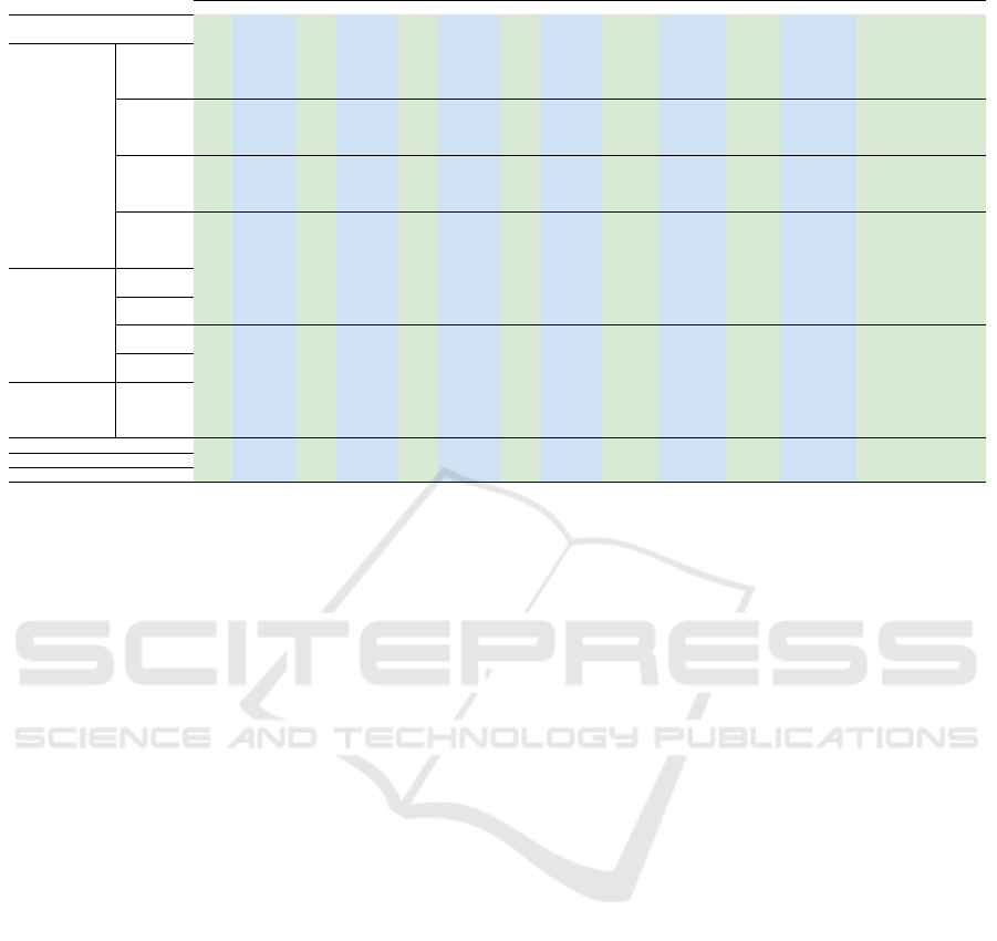
Table 5: Results for incremental training on the TAESA Benchmark.

Task 1 Task 2 Task 3 Task 4 Final Eval

% Feature mAP mAP[.50] mAP mAP[.50] mAP mAP[.50] mAP mAP[.50]

Average

mAP

Average

mAP [.50]

Ω

AP ↑ Ω

AP[.50] ↑ RSD

mAP

↓ RPD

mAP

↓

Freeze

mean 43.7 67.9 5.6 13.5 13.3 24.1 35.1 60.8 24.4 41.6 0.55 0.60 51.18 28.22

median 43.8 65.4 9.7 21 15.2 36.9 37.9 64.5 26.6 47.0 0.60 0.67 46.48 22.49

std 41.7 62.5 10.5 21.6 19.3 32.9 38.6 64.9 27.5 45.5 0.62 0.65 44.28 21.06

entropy 41.2 61.4 15.6 30.3 21 34.7 39.8 67.1 29.4 48.4 0.66 0.69 39.33 18.61

mean 44.0 69.6 5.8 13.9 11.8 23.2 35 61 24.2 41.9 0.55 0.60 51.96 28.43

median 43.3 64.7 10.5 22.5 14.8 26.3 37.2 62.6 26.5 44.0 0.60 0.63 46.52 23.93

std 41.4 64.4 10.9 22.8 19.8 34.3 38.4 64.9 27.6 46.6 0.62 0.67 43.77 21.47

entropy 41.0 61.8 16.6 31.5 22.2 37.8 39 65.9 29.7 49.2 0.67 0.71 37.77 20.25

mean 47.9 71.4 3.5 9.8 12.4 24.1 31 55.3 31.4 49.0 0.71 0.70 50.28 36.61

median 45.9 65.3 6.8 17.5 17.4 30.6 32.9 60 30.9 48.7 0.70 0.70 45.37 32.72

std 44.1 63.2 10.8 24 19.3 32.5 34.4 62.1 30.5 48.7 0.69 0.70 42.14 29.65

entropy 43.7 63.1 11.6 21.9 22.5 38.5 36.6 62.3 30.4 48.7 0.69 0.70 39.33 25.15

mean 46.2 69.9 6.8 13.9 9.9 20.7 23.3 44.9 21.6 37.4 0.49 0.54 50.95 52.35

median 45.4 68.8 8.6 22.8 15.8 29.9 25 48.5 23.7 42.5 0.53 0.61 45.62 48.88

std 44.8 68.6 13.1 27.6 18.4 33.4 25.7 49.7 25.5 44.8 0.58 0.64 40.54 47.44

entropy 45.6 67.0 13.9 28.5 19.5 33.8 28.4 53 26.8 45.6 0.61 0.65 38.43 41.92

Grad

0.1 44.2 67.8 7.5 16.6 20 34.5 37.2 64.4 27.2 45.8 0.61 0.66 44.14 23.93

0.01 29.2 65.7 8.8 18 19.9 34.1 37.9 64.7 24.0 45.6 0.54 0.65 54.84 22.49

0.1 45.7 69.7 9.7 21.4 18.8 32.6 35.2 61.7 27.4 46.4 0.62 0.67 42.16 28.02

0.01 45.4 67.9 11.2 23.1 20 34.9 37.1 64.3 28.4 47.5 0.64 0.68 40.28 24.13

0.1 47.5 70.6 9.7 23 18.5 31.6 31.5 57.7 26.8 45.7 0.61 0.66 40.97 35.58

0.01 47.0 71.6 21.1 36.5 19.2 32.6 32.3 59.4 29.9 50.0 0.67 0.72 31.96 33.95

0.1 48.7 72.9 15.6 31.1 17.7 32 28 53.1 27.5 47.3 0.62 0.68 36.09 42.74

0.01 49.2 73.5 20.4 39.4 18 32.3 27.9 53.7 28.9 49.7 0.65 0.71 31.69 42.94

MMN

25 - 44.6 68.0 5.1 12.2 17.8 31.3 33.5 60 25.3 42.9 0.57 0.62 47.36 31.49

50 - 47.3 69.7 4.2 10.1 17.4 31.7 31.5 58 25.1 42.4 0.57 0.61 46.33 35.58

75 - 49.4 72.7 6.7 15.9 15.5 28.8 28.1 52.1 24.9 42.4 0.56 0.61 44.16 42.54

90 - 48.6 72.0 10.4 18.6 14.2 26.8 13.8 32.5 21.7 37.5 0.49 0.54 42.97 71.78

Fine tuning - - 44.2 66.6 5.4 12.8 12 23.5 34.9 61.5 24.1 41.1 0.54 0.59 52.02 28.63

Experience Replay - - 46.7 71.3 21.5 37.8 24.9 40.6 42.5 71.9 33.9 55.4 0.77 0.80 27.40 13.09

Ground Truth - - 56.8 83.2 35.7 58.1 35.8 62.1 48.9 75.3 44.3 69.7 - - - -

other layer-freezing methods attained similar results,

but with less forgetting in the intermediate tasks. This

highlights the necessity to look at the big picture and

not only speciﬁc metrics based on averages.

Although the full benchmark seemed challenging

by having to deal with new classes and domains, the

initial task’s diverse and abundant data helped pre-

pare the model to learn with small adjustments in new

task scenarios. All evaluated strategies performed

better than ﬁne-tuning and MMN baselines but fell

behind the results achieved through experience re-

play. For scenarios where saving samples is not fea-

sible, a hybrid strategy involving parameter isolation

and fake labeling may help reduce the gap in perfor-

mance against replay methods. Nevertheless, when

possible, combining these methods with parameter-

isolation strategies can be seen as a promising direc-

tion for investigation.

5 CONCLUSIONS

In this paper, we discussed different ways to mitigate

forgetting when learning new object detection tasks

by using simple criteria to freeze layers and heuris-

tics for how important parameters should be updated.

We found that mining and freezing layers based on

feature map statistics, particularly on their informa-

tion entropy, yielded better results than freezing in-

dividual neurons when updating the network with

data from a single class. However, when introduc-

ing data from several classes, the simple arrangements

brought by the layer-freezing strategy were not as

successful. The layer-freezing strategies mostly out-

performed the mining of individual neurons but pre-

sented lower performance when directly compared to

more traditional and complex knowledge-distillation

methods such as ILOD and RILOD, or experience re-

play. Additionally, results also showed that applying

individual penalties to the gradients of important neu-

rons did not signiﬁcantly differ from the possibility of

freezing them.

As a future line of work, it may be beneﬁcial to ex-

plore ﬁne-grained freezing solutions that involve min-

ing and freezing individual convolutional ﬁlters based

on their internal statistics. Hybrid techniques that bal-

ance learning with the use of experience replay could

also be proposed to prevent forgetting and adapt more

quickly to new scenarios. Furthermore, it would be

useful to investigate measures of task-relatedness as

a means of deﬁning the freezing coefﬁcients among

sequential updates.

ACKNOWLEDGEMENTS

This study was funded in part by the Coordenac¸

de Aperfeic¸oamento de Pessoal de N

ıvel Superior

- Brasil (CAPES) - Finance Code 001 and by

ANEEL (Ag

encia Nacional de Energia El

etrica) and

TAESA (Transmissora Alianc¸a de Energia El

etrica

S.A.), project PD-07130-0059/2020. The authors also

would like to thank the Conselho Nacional de De-

senvolvimento Cient

ıﬁco e Tecnol

ogico (CNPq) and

the Eldorado Research Institute for supporting this re-

search.

Efﬁcient Parameter Mining and Freezing for Continual Object Detection

473

REFERENCES

Chaudhry, A., Ranzato, M., Rohrbach, M., and Elhoseiny,

M. (2018). Efﬁcient lifelong learning with a-gem.

arXiv preprint arXiv:1812.00420.

Chen, K., Wang, J., Pang, J., Cao, Y., Xiong, Y., Li, X., Sun,

S., Feng, W., Liu, Z., Xu, J., et al. (2019). Mmdetec-

tion: Open mmlab detection toolbox and benchmark.

arXiv preprint arXiv:1906.07155.

Delange, M., Aljundi, R., Masana, M., Parisot, S., Jia,

X., Leonardis, A., Slabaugh, G., and Tuytelaars, T.

(2021). A continual learning survey: Defying forget-

ting in classiﬁcation tasks. IEEE Transactions on Pat-

tern Analysis and Machine Intelligence.

Hadsell, R., Rao, D., Rusu, A. A., and Pascanu, R. (2020).

Embracing change: Continual learning in deep neural

networks. Trends in cognitive sciences.

Kirkpatrick, J., Pascanu, R., Rabinowitz, N., Veness, J.,

Desjardins, G., Rusu, A. A., Milan, K., Quan, J.,

Ramalho, T., Grabska-Barwinska, A., et al. (2017).

Overcoming catastrophic forgetting in neural net-

works. Proceedings of the national academy of sci-

ences, 114(13):3521–3526.

LeCun, Y., Denker, J., and Solla, S. (1989). Optimal brain

damage. Advances in neural information processing

systems, 2.

Li, D., Tasci, S., Ghosh, S., Zhu, J., Zhang, J., and Heck,

L. (2019). Rilod: Near real-time incremental learning

for object detection at the edge. In Proceedings of

the 4th ACM/IEEE Symposium on Edge Computing,

pages 113–126.

Li, H., Kadav, A., Durdanovic, I., Samet, H., and Graf, H. P.

(2016). Pruning ﬁlters for efﬁcient convnets. arXiv

preprint arXiv:1608.08710.

Li, W., Wu, Q., Xu, L., and Shang, C. (2018). Incremental

learning of single-stage detectors with mining mem-

ory neurons. In 2018 IEEE 4th International Con-

ference on Computer and Communications (ICCC),

pages 1981–1985. IEEE.

Li, Z. and Hoiem, D. (2017). Learning without forgetting.

IEEE transactions on pattern analysis and machine

intelligence, 40(12):2935–2947.

Lin, T.-Y., Goyal, P., Girshick, R., He, K., and Doll

ar, P.

(2017). Focal loss for dense object detection. In

Proceedings of the IEEE international conference on

computer vision, pages 2980–2988.

Liu, C. and Wu, H. (2019). Channel pruning based on

mean gradient for accelerating convolutional neural

networks. Signal Processing, 156:84–91.

Luo, J.-H. and Wu, J. (2017). An entropy-based prun-

ing method for cnn compression. arXiv preprint

arXiv:1706.05791.

Mallya, A. and Lazebnik, S. (2018). Packnet: Adding mul-

tiple tasks to a single network by iterative pruning. In

Proceedings of the IEEE conference on Computer Vi-

sion and Pattern Recognition, pages 7765–7773.

Menezes, A. G., de Moura, G., Alves, C., and de Carvalho,

A. C. (2023). Continual object detection: A review

of deﬁnitions, strategies, and challenges. Neural Net-

works.

Mirzadeh, S. I., Chaudhry, A., Hu, H., Pascanu, R., Gorur,

D., and Farajtabar, M. (2021). Wide neural net-

works forget less catastrophically. arXiv preprint

arXiv:2110.11526.

Shaheen, K., Hanif, M. A., Hasan, O., and Shaﬁque, M.

(2021). Continual learning for real-world autonomous

systems: Algorithms, challenges and frameworks.

arXiv preprint arXiv:2105.12374.

Shmelkov, K., Schmid, C., and Alahari, K. (2017). In-

cremental learning of object detectors without catas-

trophic forgetting. In Proceedings of the IEEE inter-

national conference on computer vision, pages 3400–

3409.

Tian, Z., Shen, C., Chen, H., and He, T. (2020). Fcos: A

simple and strong anchor-free object detector. IEEE

Transactions on Pattern Analysis and Machine Intel-

ligence.

ul Haq, Q. M., Ruan, S.-J., Haq, M. A., Karam, S., Shieh,

J. L., Chondro, P., and Gao, D.-Q. (2021). An incre-

mental learning of yolov3 without catastrophic forget-

ting for smart city applications. IEEE Consumer Elec-

tronics Magazine.

Wang, J., Jiang, T., Cui, Z., and Cao, Z. (2021). Filter prun-

ing with a feature map entropy importance criterion

for convolution neural networks compressing. Neuro-

computing, 461:41–54.

Wu, X., Sahoo, D., and Hoi, S. C. (2020). Recent advances

in deep learning for object detection. Neurocomput-

ing, 396:39–64.

Zenke, F., Poole, B., and Ganguli, S. (2017). Continual

learning through synaptic intelligence. In Interna-

tional conference on machine learning, pages 3987–

3995. PMLR.

Zou, Z., Shi, Z., Guo, Y., and Ye, J. (2019). Object

detection in 20 years: A survey. arXiv preprint

arXiv:1905.05055.

VISAPP 2024 - 19th International Conference on Computer Vision Theory and Applications

474