Defining KPIs for Executable DSLs: A Manufacturing System Case
Study
Hiba Ajabri
a
, Jean-Marie Mottu
b
and Erwan Bousse
c
Nantes University, LS2N Laboratory, Nantes, France
Keywords:
Domain-Specific Language, Model Execution, Key Performance Indicators, Reconfigurable Manufacturing
System.
Abstract:
Early performance evaluation is essential when designing systems in order to enable decision making. This
requires both a way to simulate the system in an early state of design and a set of relevant Key Performance
Indicators (KPIs). Model-Driven Engineering and Domain-Specific Languages (DSLs) are well suited for this
endeavor, e.g. using executable DSLs fitting for early simulation. However, KPIs are commonly tailored to
a particular system, and therefore need to be redefined for each of its variation. In light of these problems,
this paper examines how KPIs can be defined directly at the level of a DSL, thus making them available for
domain experts at the model level. We demonstrate this idea through a case study centered on a DSL to define,
simulate, and evaluate the performance of simple manufacturing systems. Models simulation is performed
by the DSL operational semantics, and yields execution traces that can then be analyzed by KPIs defined at
the DSL level. Performance results are captured using the Structured Metrics Meta-model. We illustrate the
usefulness of the proposed approach and KPIs to evaluate a simple hammer factory model and its subsequent
reconfiguration.
1 INTRODUCTION
Model-driven engineering (MDE) and Domain-
Specific Languages (DSLs) open the possibility to as-
sess the quality of a system early in the design pro-
cess. In the domain of industrial engineering and
manufacturing systems, modeling a future production
line (An et al., 2011; Kaiser et al., 2022) allows ex-
perts to thoroughly verify their design before build-
ing the actual factory. This can include checking the
structural consistency of a factory layout (e.g., are
production modules connected in a sound way?) or,
with executable models, verifying the expected be-
havior of the production line using simulation (e.g.,
is the production line able to produce the expected
product?).
An essential factor of quality of a manufacturing
system lies in its performance. Measuring the per-
formance of a system requires defining a set of rele-
vant Key Performance Indicators (KPIs) (Ferrer et al.,
2018), such as the throughput (i.e., how much a pro-
a
https://orcid.org/0009-0004-9307-6123
b
https://orcid.org/0000-0002-5245-4261
c
https://orcid.org/0000-0003-0000-9219
duction line can produce over a specified time period)
or the machine utilization (i.e., are machines always
in use, or are some machines underused?). Evaluat-
ing the performance of a system early in the design
process gives the possibility to arbitrate the choice
between different design options. A prominent ex-
ample is that of Reconfigurable Manufacturing Sys-
tems (RMS) (Koren et al., 1999), which are manufac-
turing systems designed for rapid change in order to
quickly respond to sudden market changes: when an
RMS must be reconfigured, it is crucial to evaluate
and compare the performance of the multiple consid-
ered configurations.
Performance evaluation is not an easy endeavor.
One early issue lies in the redundancy of the definition
of KPIs, since they are commonly tailored to a partic-
ular system and must therefore be redefined for each
new considered context (Ferrer et al., 2018). Defin-
ing new KPIs or adapting existing KPIs for a manu-
facturing system can quickly become a cumbersome
and error-prone task, especially in contingency situ-
ations when decisions have to be made rapidly and
efficiently.
To grapple with this issue, we examine in this pa-
per how KPIs can be defined directly at the level of a
Ajabri, H., Mottu, J. and Bousse, E.
Defining KPIs for Executable DSLs: A Manufacturing System Case Study.
DOI: 10.5220/0012361000003645
Paper published under CC license (CC BY-NC-ND 4.0)
In Proceedings of the 12th International Conference on Model-Based Software and Systems Engineering (MODELSWARD 2024), pages 169-178
ISBN: 978-989-758-682-8; ISSN: 2184-4348
Proceedings Copyright © 2024 by SCITEPRESS – Science and Technology Publications, Lda.
169

DSL, thus making them available for domain experts
at the model level. We demonstrate this idea through
a case study considering a DSL to define and evalu-
ate the performance of simple manufacturing systems.
Simulation of models is performed by the operational
semantics of the DSL, and yields execution traces that
can then be analyzed to measure KPIs defined at the
DSL level. Performance results are captured using
the Structured Metrics Meta-model (SMM) standard.
We illustrate the usefulness of the proposed approach,
DSL and KPIs to create and evaluate a simple hammer
factory model and its subsequent reconfiguration.
In the remainder, Section 2 discusses the research
background. Section 3 presents the simple manufac-
turing system as the case study, while the Section 4
discloses the approach overview and introduces the
KPI definition and computation through industrial use
cases of a simple production line. The discussion of
the related work is invoked in Section 5. Finally, con-
clusions and future works are drawn in Section 6.
2 BACKGROUND
We first present the main concepts used in our work:
manufacturing systems, Key Performance Indicators,
executable DSLs and the Structured Metrics Meta-
model.
2.1 Manufacturing Systems
Manufacturing systems (MS) are systems composed
of sequences of machines, tools, processes, and op-
erators to manufacture a specific product. Raw ma-
terials or unfinished parts are used as input to pro-
duce final manufactured parts after several assembly
and transformation operations. In this work, we con-
sider how to design a performant simple manufac-
turing system (SMS) composed of machines—which
take raw materials or unfinished products provided
on their input tray and transform them in either un-
finished or finished products—and conveyors—which
transport raw materials and products from machines
to trays. In addition, when modeling a SMS, we call
generator a specific kind of machine that does not re-
quire any inputs, and produce an output on a regu-
lar basis. Such “machines” are abstractions of stock-
piles containing raw material and products. For ex-
ample, we consider a Hammer SMS that assembles
hammers from hammer handles and hammer heads.
We can model this system using three machines: one
generator providing the handles, a second generator
providing the heads, and a third machine that given a
head and handle is able to assemble a complete ham-
mer. We connect these machines using three convey-
ors: the first two conveyors connect the generators to
a tray, the assembling machine picks parts in the tray
to assemble them, and the third conveyor collects the
hammers produced.
2.2 Key Performance Indicators
Key Performance Indicators (KPIs) are metrics that
report on the efficiency of a given system. While
some KPIs are standardized and can be applied to a
large range of domains and contexts, others are spe-
cific to a given domain, context or manufacturing sys-
tem. For instance, “communication traffic load” is
a possible KPI for resource allocations and schedul-
ing techniques in automotive applications (Latif et al.,
2016), and “traffic load” is a possible KPI to identify
the path that is most likely to experience starvation or
congestion in a conveyor belt (An et al., 2011).
In this work, we introduce two terms to help dis-
tinguishing two categories of KPIs: we call global
KPI a KPI that concerns the complete manufacturing
system, and we call local KPI a KPI that concerns
only a specific subset of the manufacturing system.
For example, a possible global KPI of a MS is the
throughput (i.e., how many products the production
line can produce over a specified time period? E.g.,
considering the Hammer SMS: how many hammers
per unit of time?), and a possible local KPI is the ma-
chine utilization (i.e., what is the percentage of use
of a given machine during the complete simulation?
E.g., considering the Hammer SMS: how much the
hammer head generator has been used?).
2.3 Structured Metrics Metamodel
The Structured Metrics Metamodel (SMM
1
) is a stan-
dard from the Object Management Group (OMG) that
defines how to represent properties, measurements,
and entities performing measurements. It specifies
concepts useful for performance analysis, such as:
• Measurement: A numerical or symbolic value as-
sociated to an entity that is assigned by a measure.
• Measurand: An entity concerned by measures
and associated to measurements.
The motivation behind using the SMM implemen-
tation is that it provides a means to store the com-
putation results, thus exempting the user from re-
computing the same model with the same input pa-
rameters. In this paper, we examine how SMM can
be applied to capture the results obtained from KPIs.
1
https://www.omg.org/spec/SMM/1.2/
MODELSWARD 2024 - 12th International Conference on Model-Based Software and Systems Engineering
170

2.4 Executable Domain-Specific
Languages
A Domain-Specific Language (DSL) is a language
providing a set of concepts fitting for a specific do-
main. We consider a DSL to be composed of two
parts. First, the abstract syntax defines the concepts of
the language and their relationships. An abstract syn-
tax can be defined as an object-oriented model called
a metamodel. Second, the execution semantics defines
how a model conforming to the abstract syntax can be
executed. Among other uses, model execution can be
an efficient way to simulate how a modeled system
would behave. We distinguish translational semantics
(i.e., compilation) and operational semantics (i.e., in-
terpretation).
In this paper, we call executable DSL (xDSL) a
DSL with a discrete event (i.e., not continuous) op-
erational semantics, and our work solely focuses on
xDSLs. We consider the operational semantics of an
xDSL to be comprised of two parts: the definition of
the possible runtime states of a model under execu-
tion, and a set of execution rules defining how such a
runtime state changes over time. One possible way to
define the runtime states is to extend the same meta-
model used to define the abstract syntax, adding new
concepts to represent the system’s dynamic behavior.
The execution rules are typically defined as endoge-
nous model transformations that modify the runtime
state of the model during its execution.
3 SIMPLE MANUFACTURING
SYSTEM xDSL CASE STUDY
In this section, we present the Simple Manufacturing
System (SMS) xDSL, which aims at modeling and
simulating simple manufacturing systems.
3.1 Abstract Syntax
3.1.1 SMS Abstract Syntax
Metamodeling of MS has been considered in sev-
eral studies, demonstrating the interest of the en-
deavor (Raith et al., 2021). However, as far as we
know, there is no standard metamodel covering ex-
haustively manufacturing systems. In our work, we
cover the main elements involved in simple manufac-
turing systems. These elements are sufficient both for
running discrete-event simulations and assessing per-
formance based on the results of these simulations.
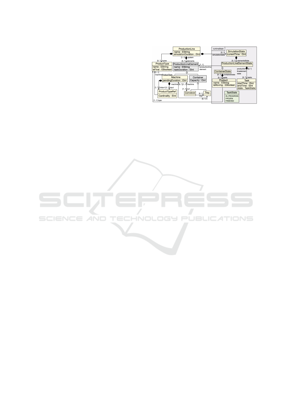
The abstract syntax of the SMS xDSL is depicted
on the left part of the Figure 1. Concepts related to
Figure 1: Abstract syntax (left part) and runtime state def-
inition (right part) of the Simple Manufacturing System
(SMS) executable DSL.
production line are defined as a set of metaclasses
and their features. Features can be either an attribute
typed by a primitive data type or a reference to an-
other metaclass.
We consider a SMS to be made of a production
line; subsequently, the root element of an SMS model
is a ProductionLine instance, which contains a set
of ProductionLineElements. A ProductionLine has a
simulationDuration that defines how long a simula-
tion of this line should last. Elements can either be
machines or containers.
A ProductionLineElement is an entity that is able
to accomplish tasks, a typical task being to move or
process products. Each ProductionLineElement has a
taskDuration value that specifies how long it takes for
this element to perform a task, and a pendingDuration
value that specifies how long the machine waits after
the execution of a task.
A Machine is a ProductionLineElement that cre-
ates products. It may consume a set of products as
input, and it produces a non-empty set of products
as output. These inputs and outputs are represented
by ProductTypeRef instances, each specifying both a
ProductType (i.e., what products are required or pro-
duced) and a cardinality (i.e., how many products of
said types are required or produced).
A Container is a ProductionLineElement that can
contain products. Two types of containers are pos-
sible: a Conveyor can transport elements, whereas a
Tray can temporarily store products to be handled. A
Machine must be connected to one or multiple Trays
to receive its input products, and must be connected
to one Conveyor where it drops output products.
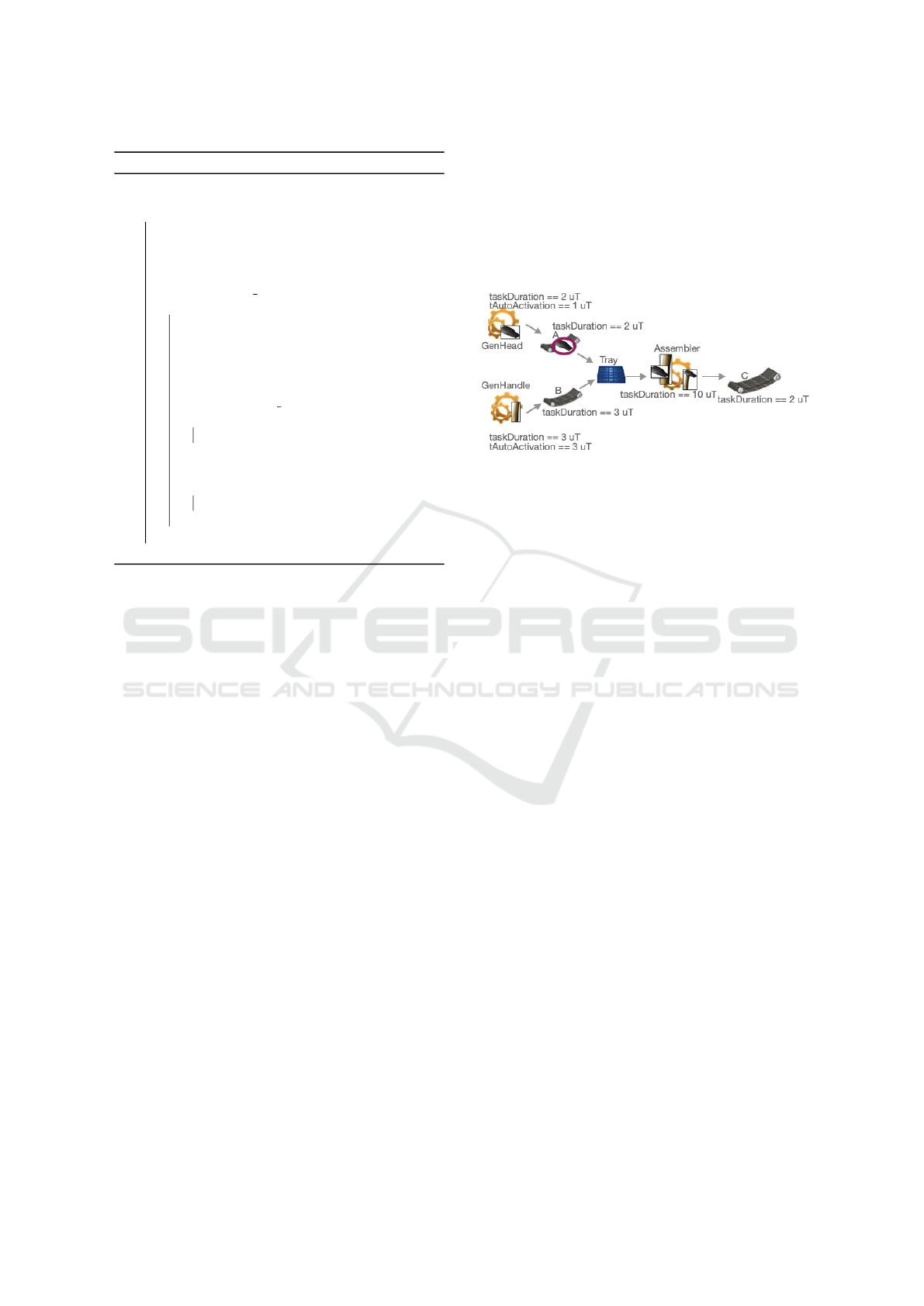
3.1.2 Example of an SMS Model: Hammer
Production Line
Figure 2 illustrates an SMS model that represents a
simple case of a manufacturing line that crafts ham-
mers. We depict the model using a graphical concrete
syntax representing the assembly of the product line.
Defining KPIs for Executable DSLs: A Manufacturing System Case Study
171

Figure 2: Hammer SMS model.
This production line contains seven elements:
three machines, three conveyors, and one tray. The
two machines GenHead and GenHandle have no in-
put but one output each, with cardinality one. They
act as generators which simulate stockpiles from
which input products are picked. They each produce
products of a specific ProductType, namely “ham-
mer head” and “hammer handle” respectively (rep-
resented with pictures framed by rectangles). Each
machine has an output conveyor, to deliver each gen-
erated product. The conveyors, in turn, are associated
to the same tray. The tray simulates temporary stor-
age as the input of the next machine. The Assembler
machine retrieves one head and one handle from the
tray to assemble them, and produces a hammer. The
Assembler cannot start producing a hammer unless it
has a handle and a head as input. Once a hammer is
generated, it will be placed on the conveyor linked to
the Assembler’s output, which is the last element in
the chain.
In this production line system, we presume that
the two generator machines (i.e., GenHead and Gen-
Handle) may produce an infinite number of heads and
handles. We set the task durations and pending dura-
tions of the machines GenHead and GenHandle. The
Assembler has a task duration, but no pending dura-
tion, meaning that it will work as soon as the required
product parts are available in the tray.
3.2 Operational Semantics
We define the operational semantics of the SMS
xDSL, which will then allow the simulation of any
SMS model, such as the Hammer SMS.
3.2.1 Discrete-event Simulation
In our work, we rely on discrete event simula-
tion (Adam et al., 2011) to define when the runtime
state is updated. Figure 3 illustrates such a discrete
event simulation of the Hammer SMS model. The
horizontal lines represent the timeline of each produc-
tion line element that has a behavior (the machines
Figure 3: State capture and time advancement based on the
discrete event simulation of the Hammer SMS.
and the conveyors). Lines with brackets represent a
running task. The red circles represent when the run-
time state is updated: the endings of the tasks.
The execution of the system embodies events that
occur simultaneously or sequentially. In succes-
sive operation chains that happen systematically, after
each completion of a task, other tasks are considered
to be triggered if possible (represented with curved
dashed arrows in Figure 3).
3.2.2 SMS Runtime State Definition
The right part of Figure 1 depicts the runtime state
definition of the SMS xDSL. It is defined in a sepa-
rate package of the SMS xDSL metamodel, and in-
troduces additional metaclasses and features defining
the runtime states of the different language concepts
shown in the abstract syntax (left part of Figure 1).
An SMS model under execution contains a Simu-
lationState, the latter containing a set of Production-
LineElementState for each ProductionLineElement.
Each ProductionLineElementState has a reference
to its specific ProductionLineElement, and contains a
list of Task elements representing all ongoing tasks
performed by the element. A Task has a start time
(as an Integer), an end time (as an Integer) and a task
state (which can be either IN PROGRESS, FROZEN,
or FINISHED). The currentTime of the simulation is
changed each time the runtime state is updated, which
occurs when a task of an element is completed and/or
it starts. We also define ContainerState to represent
that a container may contain Product elements. Each
product has a reference to a specific ProductType of
the model. The attribute isMoving represents the pos-
sibility that a product may be currently in movement
on a conveyor belt.
The initial runtime state of the model is created
before the execution starts. We choose an initial run-
time state where all containers are empty, and no tasks
yet exist. This state is the one of the example model
shown in Figure 2.
3.2.3 SMS Execution Rules
We defined a set of execution rules that specify how
the runtime state of a given SMS model changes over
MODELSWARD 2024 - 12th International Conference on Model-Based Software and Systems Engineering
172

Algorithm 1: Machine :: start() execution rule.
Inputs:
simulationState : SimulationState
machine : Machine
currentTime : Integer
begin
if machine.verifyIfMachineCanStart(
simulationState, currentTime) then
task ←
machine.createOrGetTask(simulationState,
currentTime);
machine.initializeTaskValues(currentTime,task);
machine.consumeInputsIfNeeded(
simulationState);
end
end
time during a simulation, following the principles of
discrete-event simulation:
• ProductionLine::initialize(): Prepare the initial
runtime state by creating one SimulationState, one
ContainerState per Container, and one Produc-
tionLineElementState per Machine.
• Conveyor::start(): Given a Conveyor, examine
whether the conditions are met for the conveyor
to create and possibly start new Tasks. This re-
quires the input Machine to have finished prepar-
ing a product, and space available on the conveyor
(as given by its capacity).
• Machine::start(): Given a Machine, examine
whether the conditions are met for the machine
to create and start new Tasks. This requires input
products to be available, and requires the machine
to be ready to work. When a task is created, the
required input products are removed from the in-
put tray.
• Conveyor::finishTask(): Given a Conveyor and a
Task, ends this task, which moves the product on
the container into the output Tray.
• Machine::finishTask(): Given a Machine and a
Task, ends this task, which creates output prod-
ucts as specified in the machine.
• ProductionLine::main(): Executes a Production-
Line until the end of the simulation. This is the
only execution rule that must be called to run
a simulation, which will trigger other execution
rules as it goes by.
We give a simplified pseudocode description of a
subset of these rules:
Machine::start(). Algorithm 1 shows the Ma-
chine::start(currentTime : Integer) execution rule. In
Algorithm 2: Machine :: f inishTask() execution rule.
Inputs:
simulationState : SimulationState
task : Task
machine : Machine
begin
produceOutputProducts(simulationState,machine);
task.state= FINISHED;
end
this part, we suppose we have the following utility
functions available:
• Machine::verifyIfMachineCanStart(): Verify the
eligibility of the machine to create and start a task,
which is achieved by checking the following con-
straints: (1) the presence of sufficient input prod-
ucts if required; (2) the machine is not in an active
state (i.e., does not have a running task); (3) the
machine is not frozen (i.e., does not have a task
in a frozen state); (4) the attached conveyor will
have space to transport the produced output prod-
ucts ; and (5) the currentTime is the right time for
the machine to begin its work (particularly for the
machines requiring no inputs (i.e., generators)).
• Machine::initializeTaskValues(): Initialize the at-
tributes of the task (i.e., endTime, state) with val-
ues.
• Machine::consumeInputsIfNeeded(): A machine
requiring inputs consumes the needed inputs to
produce the expected output products.
Whenever a production line element is asked to
work, a task associated to its ProductionLineEle-
mentState is considered. Particularly for machines re-
quiring no inputs (e.g., a generator such as GenHead,
Figure 2), two tasks are created : the first is meant to
work at the current time, and the second is prepared
to work for the coming runtime states (i.e., the task
is prepared by calculating its expected start time). A
conveyor may have several tasks running at the same
time, each one corresponding to moving one product
from a machine to a tray, several ones can be moved
at the same time (w.r.t. its capacity).
Machine::finishTask(). Algorithm 2 shows the Ma-
chine::finishTask() execution rule. In this part, we
suppose we have a utility function named:
• Machine::produceOutputProducts(): At this step,
the machine can actually produce output products
and deliver them on the attached conveyor.
ProductionLine::main(). Algorithm 3 shows the
main execution rule that comprises the main loop of
Defining KPIs for Executable DSLs: A Manufacturing System Case Study
173

Algorithm 3: ProductionLine :: main() execution rule.
Inputs:
ProductionLine: the model of the system
begin
simulationState ← initialize();
startGenerators(ProductionLine,simulationState);
while simulationState.tasks().exists(task |
task.state = IN PROGRESS) ∧ currentTime <
ProductionLine.simulationDuration do
currentTime ←
computeNextTime(simulationState);
ProductionLine.simulationstate.currentTime
= currentTime;
foreach (task in simulationState.tasks() |
task.state = IN PROGRESS ∧
task.endTime = currentTime) do
task.finishTask(currentTime);
end
foreach
element ∈ ProductionLine.elements do
element.start(currentTime);
end
end
end
the system execution. This single rule is used to start
the execution of a given SMS model, and triggers
other execution rules while it unrolls. Since, by de-
fault, all machines are stopped and do nothing, an ini-
tialisation stage is performed by using the following
utility function :
• ProductionLine::startGenerators(): starting (us-
ing the start execution rule) all machines that do
not require any input products, i.e., generators.
The products continuously delivered by generators
will then eventually trigger a simple “chain reaction”,
since other machines will be eventually triggered by
the presence of input products. Once the initialization
is complete, the main execution loop starts, and will
continue while tasks occur and while the simulation
target duration has not been reached. During a loop
iteration, we start by “jumping” to the next instant
where something occurs in the simulation, i.e., either
the end of an ongoing task or the start of a coming
prepared task. This is achieved by a utility function
named computeNextCurrentTime:
• ProductionLine::computeNextCurrentTime():
Look over all ongoing and the coming prepared
tasks, and searching for the smallest scheduled
end or start time.
We thereby update the currentTime of the simulation,
with this value. Then, we find all tasks that should end
at the new current time value, and trigger the finish-
Task() execution rule on each of these tasks. Depend-
ing on the type of the element performing the task,
the finishTask() execution rule might move an element
(e.g., in the case of a conveyor) or produce an out-
put element (e.g., in the case of a machine). Finally,
the start execution rule is triggered on all elements,
which will create new tasks for elements if conditions
are met, as explained previously.
Figure 4: CurrentTime 2 uT during the execution of the
Hammer SMS model.
Example of SMS Model Execution. For instance,
let’s execute the Hammer SMS model illustrated
in Figure 2. The start time is set to 0, it is the
currentTime of the first runtimeState (the first red cir-
cles, from the left in Figure 3). Then, the GenHead
and GenHandle are requested to start. Being ma-
chines requiring no input, two tasks are instantiated
and associated to the ProductionLineElementState of
these generator machines. The two tasks have a state
in progress. The loop (in Algorithm 3) runs as long
as there are tasks in progress. The GenHead task
will finish at an instant equal to 2 units of time (uT),
whereas the GenHandle task will finish at 3 uT. There-
fore, the next currentTime is computed, being at this
stage 2 uT. Next, the GenHead task finishes as it is
in progress, i.e., means that the GenHead produces a
head and delivers it to the Conveyor A. Figure 4 high-
lights this runtime state with this produced head sur-
rounded with a red circle. Then, we look at potential
tasks to start. At that currentTime (at 2 uT, Figure 4),
the Conveyor A can start, having received a product
to move (i.e., the head produced by GenHead). At
this point, the capture of the runtimeState at 2 uT has
been successfully built. The next currentTime is com-
puted, it is 3 uT, the endTime of the GenHandle task.
This handle generator delivers a handle product to the
Conveyor B, which can have a task starting. The exe-
cution will continue in this direction.
MODELSWARD 2024 - 12th International Conference on Model-Based Software and Systems Engineering
174

4 DEFINITION AND
COMPUTATION OF
LANGUAGE-LEVEL KPIs
This section presents how we define and compute
language-level KPIs for the SMS xDSL using exe-
cution traces produced by the operational semantics.
The implementation of the xDSL, of a SMS KPI Cat-
alog and of a GUI is provided in a dedicated public
GitLab repository
2
.
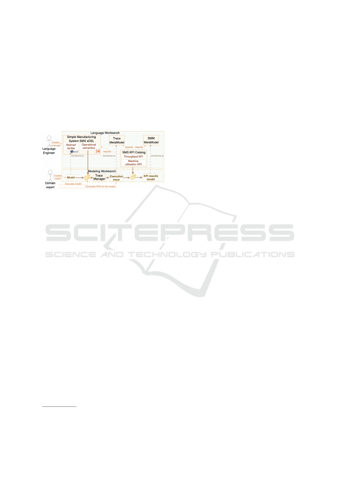
Figure 5: KPI definition and computation process.
4.1 Overview
Figure 5 depicts the KPI definition and computation
process for the SMS xDSL. At the top, the language
engineer uses the language workbench to create both
the SMS xDSL (as presented in the previous section),
and a set of relevant KPIs specific to the SMS xDSL.
Each of these KPIs is registered in a catalog consid-
ered as an SMS KPI Catalog, and it relies on the con-
cepts of the xDSL for its definition (e.g., counting the
amount of finished products), and expect as input data
an execution trace of an SMS model.
At the bottom, the domain expert (i.e., the user
of the SMS xDSL) creates an SMS model using the
modeling workbench. She can then execute the SMS
model to simulate the manufacturing system behavior,
which yields an execution trace model that conforms
to the trace metamodel. In this paper, we do not de-
tail how these traces are produced, and we assume a
trace manager is available for this task. This trace
manager observes the complete simulation, and takes
a snapshot of the model state after each simulation
step. In the case of SMS, a simulation step consists
of simulating all the elements of the system until the
next instant. Finally, the domain expert is able to use
the language-level pre-defined KPIs available in the
SMS KPI Catalog to evaluate the performance of her
model. This computation relies on the execution trace
produced by the operational semantics, and yields a
set of KPI results persisted in a model that conforms
2
https://gitlab.univ-nantes.fr/rodic/simpleplsdsl/
to the standard SMM metamodel. The domain expert
can then assess the performance of the manufacturing
system at the model level. Therefore, she can com-
pare the evaluation results of several design alterna-
tives by changing only the model.
4.2 Definition of an SMS KPI Catalog
In our approach, an SMS KPI Catalog defines differ-
ent performance indicators that the user may select
when assessing the performance of a system. Each
KPI has its own specific formula, which is written
as a software program that is able to query an execu-
tion trace model and computes the measurements. We
consider the following two KPIs for the SMS xDSL:
• Throughput: a global KPI giving the amount of
final products produced at the end of the simu-
lation, divided by the duration of the simulation,
i.e., the production speed of the system.
• Machine Utilization: a local KPI giving the per-
centage of operating duration of one element of
the SMS model (to be opposed to the pending du-
ration).
The KPIs presented in the article are assuredly not
exhaustive of all KPIs used in the industrial domain,
since our objective was to present a proof of concepts
and not to iterate on all existing KPIs. Nevertheless,
these examples of KPIs constitutes fertile ground for
other KPIs as we can apply the same process: defining
other KPIs in the language workbench to be used by
the domain expert in the modeling workbench on new
models of a system.
Algorithm 4 shows the KPI formula for the
throughput KPI. While this formula takes as input
a complete execution trace—as all KPI formulas in
our approach— and the type of the final product that
the user requests its throughput. This capability gives
the proposed approach a parameterization feature: the
user can parameterize the KPI computation by spec-
ifying which KPI to compute, on/or which element
to consider. Note that this KPI in particular only re-
quires looking at the last execution state captured in
the trace. The results are captured in an SMM model,
and as such a significant part of the logic is dedicated,
we suppose we have two utility functions to assist the
creation and modification of the SMM model:
• initializeSMMmodel() : Initilize the SMM model,
and all elements needed (e.g., SMM Library,
SMM observation).
• storeComputedKPIValue() : Create a SMM Mea-
surement element to store the computed through-
put value.
Defining KPIs for Executable DSLs: A Manufacturing System Case Study
175

Algorithm 4: Throughput KPI formula.
Inputs:
executionTrace: the trace of the execution of the
model
SMMmodel: SMM model where to store the output
type : type of which the user wants its throughput
begin
SMMmodel ← initializeSMMmodel();
S ← executionTrace.states.last.currentTime;
N ← 0;
foreach container ∈ ExecutionTrace.finalState
do
count ← 0;
foreach part ∈ container.getParts() do
if part.getType().equals(type) then
count + +;
end
end
if count > 0 then
N ← N + count;
end
end
storeComputedKPIValue(SMMmodel, N/S);
end
4.3 KPI Computation on Several
Models
Once the language engineer has defined KPIs in the
language workbench, the domain expert can focus on
the models of the systems she wants to assess the per-
formance. In this section, we illustrate how one can
compute the KPIs on several versions of a system, by
changing its models but without requiring to imple-
ment the KPI for each model again.
Firstly, We execute the Hammer SMS model al-
ready presented in Figure 2 with a simulation dura-
tion of 419 uT and we obtain an execution trace. We
then select the throughput KPI formula considering
the hammer products, shown in Algorithm 4. The
computation returns that 41 hammer products have
been produced, hence the computed throughout KPI
value is 41/419 ' 0.1, i.e., on average 0.1 hammer is
produced for 1 uT. This measurement is persisted in a
KPI results model.
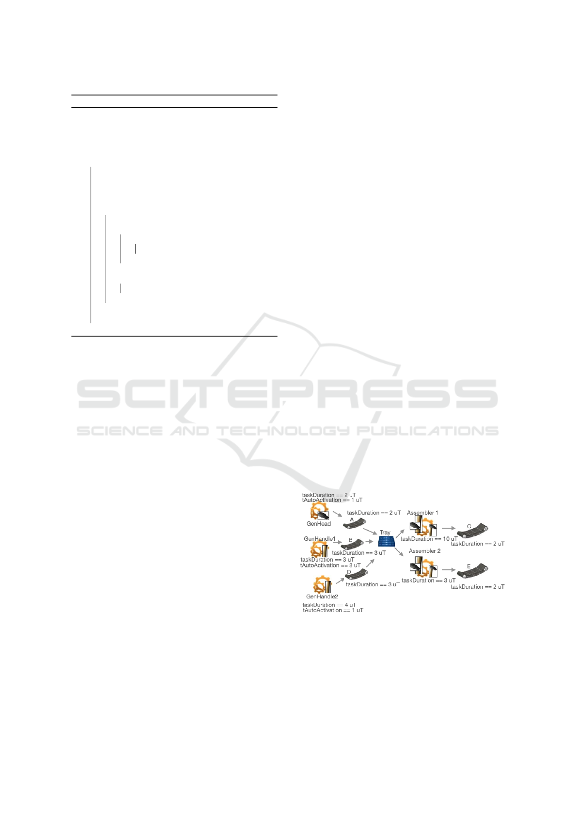
Thanks to this analysis, it is secondly possible to
consider another design of the hammer production
line. The domain expert may focus on increasing
the throughput by adding another generator of han-
dles and another assembler, and we therefore end up
with two assemblers that work in parallel as shown in
Figure 6. We run a new simulation with a duration
of 419 uT for this second version, and computing the
throughput KPI on hammer products, we obtain this
time a value of 138/419 ' 0.3 hammer produced for
1 uT. Note that because multiple assemblers are using
the same input tray, the simulator will randomly select
which assembler is allowed to pick products from the
tray, which may induce inherent differences from one
simulation to another (e.g., 137 produced hammers
instead of 138).
Starting again from the first version (Figure 2),
we can explore another scenario where we introduce
drastic capacity limits in the different containers of
the system (i.e., a capacity equal to 1 for each con-
veyor and equal to 2 for the tray). This third version
of the model is shown in Figure 7. We run a simula-
tion for 419 uT, but quickly observe that the system is
stuck at 27 uT after producing only 2 hammers. The
explanation lies in the capacity assigned to different
containers. The first container that blocks the produc-
ing chain is the Conveyor C as its capacity is restricted
to one product, which said that the Assembler activity
will be suspended after producing the first hammer.
Since the Tray capacity also can not exceed two prod-
ucts, this will paralyze the Conveyor A and B activi-
ties, which will be raised to the generators level. An-
other situation that may also occur is ending up with
either two hammer heads or two hammer handles in
the tray, which makes it impossible for the assembler
to continue, leading to a deadlock. The resulting KPI
throughout value is close to zero (2/419).
This section illustrates that, once the SMS xDSL
and its SMS KPI Catalog are defined and imple-
mented by a language engineer, a domain expert can
focus on modeling several models of a hammer pro-
duction line and compute automatically their KPI.
The proposed approach helps a domain expert to re-
duce her effort by providing relevant information,
thus supporting rapid decision-making when recon-
figuring a system for instance.
Figure 6: Second version of the Hammer Production Line,
with added generator and assembler.
MODELSWARD 2024 - 12th International Conference on Model-Based Software and Systems Engineering
176

Figure 7: Third version of the Hammer Production Line,
with drastic container capacity limits.
5 RELATED WORK
In this section, we report on existing work on the use
of MDE and DSLs in the manufacturing domain, and
on performance evaluation.
5.1 Use of MDE and DSLs in the
Manufacturing Domain
There have been many ventures to use MDE and
DSLs in the manufacturing domain. Some specific
approaches propose MDE-based solutions adapted for
specific sorts of manufacturing systems (An et al.,
2011; Kaiser et al., 2022), while more general ap-
proaches propose to generate code from models in or-
der to run simulations (Berruet et al., 2007; Lallican
et al., 2007; Prat et al., 2017). There is also flourish-
ing work on the use of MDE to produce digital twins
(Bordeleau et al., 2020; Eramo et al., 2022) (i.e., a
digital representation of a running cyber-physical sys-
tem able to predict its behaviors and make decisions
accordingly), and existing applications to manufactur-
ing systems (Lugaresi and Matta, 2021).
Overall, compared to existing work, the DSL
shown in the present paper only focuses on very sim-
ple manufacturing systems at a very high-level of ab-
straction (e.g., each machine or element is represented
as a black-box, and everything is discrete), with a
focus on designing the physical layer of a manufac-
turing system. While most of these approaches aim
to run simulations, they do not investigate how and
at which abstraction level KPIs should be defined.
Through a simple case study, our objective was to in-
vestigate how to reduce the effort of the domain ex-
pert, related to KPI definition and performance evalu-
ation using language-level KPIs.
5.2 Performance Evaluation Using
MDE and DSLs
In the manufacturing domain, Lugaresi et al. (Lu-
garesi and Matta, 2021) propose to automatically gen-
erate a digital twin from an existing system, and to
use this digital to estimate the performance of the real
system. Compared to our work, while the authors de-
fine some KPIs, the work is not focused on how these
KPIs are defined nor at which level of abstraction they
should be defined.
Outside the manufacturing domain, probably the
contribution closest to ours is from B
´
eziers La Fosse
et al. (la Fosse et al., 2020) (and with one co-author
participating to the present paper), who propose to de-
fine energy language-level consumption metrics for
each concept of a given DSL. These metrics are then
used to estimate the energy consumption of a system
modeled and executed with said DSL. In a way, this
work provides the means to generalize a specific sort
of KPI (energy consumption) directly at the language
level, while our work is interested in all sorts of KPIs
at the language level, with a specific application to
manufacturing systems.
With the same logic, Monahov et al. (Monahov
et al., 2013) propose to integrate a DSL for KPI’s def-
inition and computation into Enterprise Architecture
Management (EAM) tools to quantify Enterprise Ar-
chitecture (EA) characteristics, thus enabling assess-
ment of EA and measuring the level of goal achieve-
ment for EAM. The designed language allows domain
experts to define KPIs through the implementation of
custom functions and evaluate them. Nonetheless,
the designed language was more technically oriented
than conceptually engineered; it does not present any
concepts constructed around KPIs or performance no-
tions. Otherwise, it was mainly founded on the ag-
gregation of query languages and primitive functions,
which results in a query language that may prove dif-
ficult to use for domain experts with modest program-
ming knowledge. Compared to our approach, we look
to reduce the effort related to the definition of KPIs
on the model level, i.e., the domain experts are not
requested to write code to query and extract neces-
sary data from the concern model, instead they can
easily select KPIs desired from the SMS KPI Cata-
log, which is predefined at the language level, to get
the expected results. Certainly, the domain experts
can enrich the SMS KPI Catalog with relevant KPIs
according to the application domain (Monahov et al.,
2013); nevertheless, the process of feeding this cata-
log should not amortize the decision-making process.
Moreover, our approach presents an offline eval-
uation process implemented thanks to the execution
Defining KPIs for Executable DSLs: A Manufacturing System Case Study
177

trace mechanism, which separates the performance
evaluation from the runtime execution and thus per-
mits domain experts to evaluate the model whenever
it is required.
6 CONCLUSION
This paper examined how KPIs can be defined di-
rectly at the level of a DSL, thus making them avail-
able for domain experts at the model level. This idea
was presented through a case study centered on a DSL
to define, simulate, and evaluate the performance of
simple manufacturing systems. We defined a set of
KPIs for this DSL, and illustrated their use with an
example of a simple manufacturing system.
As this paper presents early results from our
ongoing work, many future research directions are
possible. Instead of relying on a generic meta-
programming language, the definition of KPIs could
be facilitated using a dedicated KPI definition meta-
language. This work could also be generalized to be
applicable to any executable DSL for which perfor-
mance measurement would be relevant.
ACKNOWLEDGEMENTS
This work was supported by the French National Re-
search Agency (ANR) [grant number ANR 21 CE10
0017].
REFERENCES
Adam, M., Cardin, O., Berruet, P., and Castagna, P. (2011).
Proposal of an Approach to Automate the Generation
of a Transitic System’s Observer and Decision Sup-
port using Model Driven Engineering. IFAC Proceed-
ings Volumes, 44(1):3593–3598.
An, K., Trewyn, A., Gokhale, A., and Sastry, S. (2011).
Model-Driven Performance Analysis of Reconfig-
urable Conveyor Systems Used in Material Handling
Applications. In 2011 IEEE/ACM Second Interna-
tional Conference on Cyber-Physical Systems, pages
141–150, Chicago, IL, USA. IEEE.
Berruet, P., Lallican, J. L., Rossi, A., and Philippe, J. L.
(2007). Generation of control for conveying systems
based on component approach. In 2007 IEEE Interna-
tional Conference on Systems, Man and Cybernetics.
IEEE.
Bordeleau, F., Combemale, B., Eramo, R., van den Brand,
M., and Wimmer, M. (2020). Towards model-driven
digital twin engineering: Current opportunities and
future challenges. In Communications in Computer
and Information Science, pages 43–54. Springer In-
ternational Publishing.
Eramo, R., Bordeleau, F., Combemale, B., van den Brand,
M., Wimmer, M., and Wortmann, A. (2022). Concep-
tualizing digital twins. IEEE Software, 39(2):39–46.
Ferrer, B. R., Muhammad, U., Mohammed, W., and Las-
tra, J. M. (2018). Implementing and visualizing ISO
22400 key performance indicators for monitoring dis-
crete manufacturing systems. Machines, 6(3):39.
Kaiser, B., Reichle, A., and Verl, A. (2022). Model-based
automatic generation of digital twin models for the
simulation of reconfigurable manufacturing systems
for timber construction. Procedia CIRP, 107:387–
392.
Koren, Y., Heisel, U., Jovane, F., Moriwaki, T., Pritschow,
G., Ulsoy, G., and Van Brussel, H. (1999). Re-
configurable Manufacturing Systems. CIRP Annals,
48(2):527–540.
la Fosse, T. B., Tisi, M., Mottu, J.-M., and Suny
´
e, G. (2020).
Annotating executable DSLs with energy estimation
formulas. In Proceedings of the 13th ACM SIGPLAN
International Conference on Software Language En-
gineering. ACM.
Lallican, J. L., Berruet, P., Rossi, A., and Philippe, J. L.
(2007). A component-based approach for convey-
ing systems control design. In 4th International
Conference on Informatics in Control, Automation
and Robotics ICINCO 2007, pages 329–336, Angers,
France.
Latif, K., Selva, M., Effiong, C., Ursu, R., Gamatie, A., Sas-
satelli, G., Zordan, L., Ost, L., Dziurzanski, P., and
Indrusiak, L. S. (2016). Design space exploration for
complex automotive applications: an engine control
system case study. In Proceedings of the 2016 Work-
shop on Rapid Simulation and Performance Evalua-
tion: Methods and Tools, pages 1–7, Prague Czech
Republic. ACM.
Lugaresi, G. and Matta, A. (2021). Automated manufac-
turing system discovery and digital twin generation.
Journal of Manufacturing Systems, 59:51–66.
Monahov, I., Reschenhofer, T., and Matthes, F. (2013).
Design and Prototypical Implementation of a Lan-
guage Empowering Business Users to Define Key
Performance Indicators for Enterprise Architecture
Management. In 2013 17th IEEE International En-
terprise Distributed Object Computing Conference
Workshops, pages 337–346, Vancouver, BC, Canada.
IEEE.
Prat, S., Cavron, J., Kesraoui, D., Rauffet, P., Berruet,
P., and Bignon, A. (2017). An Automated Gen-
eration Approach of Simulation Models for Check-
ing Control/Monitoring System. IFAC-PapersOnLine,
50(1):6202–6207.
Raith, C., Woschank, M., and Zsifkovits, H. (2021). Meta-
modeling in Manufacturing Systems: Literature Re-
view and Trends. In Proceedings of the International
Conference on Industrial Engineering and Operations
Management, Singapore.
MODELSWARD 2024 - 12th International Conference on Model-Based Software and Systems Engineering
178