Comparing Global and Local Weights in Multi-Criteria
Decision-Making: A COMET-Based Approach
Andrii Shekhovtsov
1 a
and Wojciech Sałabun
1,2 b
1
National Telecommunications Institute, ul. Szachowa 1, Warsaw 04-894, Poland
2
West Pomeranian University of Technology in Szczecin, ul.
˙
Zołnierska 49, 71-210 Szczecin, Poland
Keywords:
MCDA, COMET Method, Local Weights Identification, Simulation Experiment, Linear Regression.
Abstract:
In the multi-criteria decision-making (MCDM) domain, decision-makers encounter the challenge of consid-
ering multiple criteria with varying importance. While numerous methods exist to determine global weights,
less attention has been given to identifying local weights for individual alternatives. Unlike global weights, lo-
cal weights indicate the relevance of individual criteria in the context of a specific alternative. Global weights
assume a constant linear dependence of substitutability throughout the domain, where local weights indicate a
local dependence, depending on the value of all attributes of a given alternative.
This paper demonstrates the usage of Characteristic Objects METhod (COMET) to determine local criteria
weights and provides simulation results to show the differences in those weights. By understanding the signif-
icance of criteria for specific alternatives and their impact on the overall evaluation, local weights contribute
to a more comprehensive and reliable ranking. This paper presents the necessary methodologies, describes
the pseudocode algorithm, and showcases two examples of two COMET models and a simulation that utilizes
the ESP-COMET approach. The simulation results highlight generalized results showing the importance of
identifying local weights.
1 INTRODUCTION
In every decision problem, one or more different cri-
teria are included. Decisions are usually made based
on these criteria, which can be more or less obvious
to the decision-maker. In complex decision-making
problems, the decision-maker can be forced to han-
dle multiple opposing criteria, which can be difficult
to do. In this case, the expert can use the methodolo-
gies and approaches utilized in the Multi-Criteria De-
cision Analysis (MCDA) domain, where the decision
maker should identify a set of alternatives and criteria.
However, further use of MCDA methods requires the
definition of the criteria weights (Mahmoody Vanolya
and Jelokhani-Niaraki, 2021). Many different meth-
ods allow one to identify global weights in decision
problems, such as Analytic Hierarchy Process (AHP)
(Saaty, 2004), RANking COMparison (RANCOM)
(Wi˛eckowski et al., 2023b), and others (Biswas et al.,
2022; Lipka and Szwed, 2021). However, little atten-
tion is paid to identifying local weights for individual
a
https://orcid.org/0000-0002-0834-2019
b
https://orcid.org/0000-0001-7076-2519
alternatives (Choo et al., 1999; Ullah et al., 2018).
Local weights play a vital role in the conduct
of a thorough analysis of decision problems, crite-
ria, and alternatives, as evidenced by previous studies
(Elanchezhian et al., 2010; Wi˛eckowski et al., 2023a).
They address the critical question of the relative im-
portance of specific criteria for particular alternatives
and how much they influence the overall evaluation
of the considered alternatives. The determination of
local criteria not only aids in gaining a deeper un-
derstanding of the decision problem but also clarifies
the prerequisites that the alternatives must meet. For
example, they allow one to adjust the importance of
specific attributes within the context of a given al-
ternative. In contrast, global weights maintain uni-
form importance for each criterion. To illustrate, con-
sider the body temperature problem of a patient with
COVID-19, where temperature is one of the basis of
diagnosis. The relevance of body temperature in the
context of COVID-19 patients is meaningful only in
specific circumstances, as excessively high tempera-
tures can potentially harm proteins. This means that
normal temperature levels have no significant impact
on the severity of COVID-19, whereas high tempera-
470
Shekhovtsov, A. and Sałabun, W.
Comparing Global and Local Weights in Multi-Criteria Decision-Making: A COMET-Based Approach.
DOI: 10.5220/0012360700003636
Paper published under CC license (CC BY-NC-ND 4.0)
In Proceedings of the 16th International Conference on Agents and Artificial Intelligence (ICAART 2024) - Volume 3, pages 470-477
ISBN: 978-989-758-680-4; ISSN: 2184-433X
Proceedings Copyright © 2024 by SCITEPRESS – Science and Technology Publications, Lda.

tures become very important and are more important
when they increase (Yombi et al., 2020).
The Characteristic Objects METhod is an MCDA
method utilizing the fuzzy theory and rule-based
system to provide reliable and accurate rankings
of the alternatives based on the expert’s knowledge
(Sałabun, 2015). It has many extensions (Faizi et al.,
2018; Faizi et al., 2017) and has proven its robust-
ness in many application fields, such as energetic
(Kizielewicz et al., 2020), agriculture (Habeeb et al.,
2022), sport (Wi˛eckowski and Dobryakova, 2021)
and other (Kozlov and Norek, 2021).
The novelty and main contribution of the paper is
to demonstrate the algorithm for the identification of
local and global weights on the simple examples and
provide a simulation based on the ESP-COMET ap-
proach, which shows how significant and useful the
knowledge about local weights can be in the case
of personalized decision-making when dealing with
complex nonlinear expert preferences. The simula-
tion based on the ESP-COMET approach clearly em-
phasizes the significance of knowledge about local
weights when making personalized decisions when
dealing with complex nonlinear expert preferences.
This is important because it highlights that in a non-
linear model, the importance of individual criteria
changes.
The rest of the paper is structured as follows: In
Section 2, we describe all the necessary methodolo-
gies required to understand the described Study Case.
In the next part of the paper, we present two examples
that utilize the COMET method to determine the lo-
cal weights of the criteria: the example with a linear
expert function is shown in Section 3.1, and the exam-
ple with a nonlinear expert function is shown in Sec-
tion 3.2. To simulate nonlinear expert preferences, we
utilize the recently proposed ESP-COMET approach.
Next, we present a simulation that repeats the exper-
iment described in Section 3.2 to obtain generalized
differences between local and global weights. The
simulation results are presented in Section 3.3. Fi-
nally, in Section 4, we conclude our work and propose
future research directions.
2 PRELIMINARIES
This section provides the information necessary to
understand the presented methodology. In Section
2.1, we briefly describe the Characteristic Objects
METhod, which will be used as the main instru-
ment to identify the local weights of the alternatives.
Next, we explain the ESP-COMET procedure and
how it can be used to simulate non-linear expert pref-
erences. We also describe the recently introduced
Weighted Similarity Coefficient WSC
2
, allowing us to
measure the distance between different weights effi-
ciently. The description of the W SC
2
coefficient can
be found in Section 2.3.
2.1 The Characteristic Objects Method
The Characteristic Objects Method (COMET) is
the MCDA method that was initially proposed by
(Sałabun, 2015) as a more reliable and robust sub-
stitution of classical MCDA methods. It allows the
model expert preferences with different levels of com-
plexity utilizing the Matrix of Experts Judgements
(Kizielewicz et al., 2021). The algorithm of the
COMET method is completely free of rank reversal
paradox because of the independent evaluation of ev-
ery alternative. The implementation of the COMET
method can be found in the easy-to-use Python library
of the MCDA methods called pymcdm (Kizielewicz
et al., 2023). The algorithm is fully explained in the
other publications, such as (Sałabun, 2015), therefore
we will provide only a short version.
Step 1. Define the Space of the Problem – the expert
determines the dimensionality of the problem by se-
lecting the number r of criteria, C
1
,C
2
,...,C
r
. Then,
the set of fuzzy numbers for each criterion C
i
should
be selected.
Step 2. Generate Characteristic Objects – The charac-
teristic objects (CO) are obtained by using the Carte-
sian Product of fuzzy numbers cores for each criteria
as follows.
Step 3. Rank the Characteristic Objects – the expert
determines the Matrix of Expert Judgment (MEJ).
The MEJ matrix contains results of comparing char-
acteristic objects by the expert, where α
i j
is the re-
sult of comparing CO
i
and CO
j
by the expert. The
function f
exp
denotes the mental function of the ex-
pert represented as (1). Afterward, the vertical vector
of the Summed Judgments (SJ) is obtained as follows
(2).
α
i j
=



0.0, f
exp
(CO
i
) < f
exp
(CO
j
)
0.5, f
exp
(CO
i
) = f
exp
(CO
j
)
1.0, f
exp
(CO
i
) > f
exp
(CO
j
)
(1)
SJ
i
=
∑
t
j=1
α
i j
(2)
Finally, values of preference are approximated for
each characteristic object. As a result, the vertical
vector P is obtained, where i − th row contains the
approximate value of preference for CO
i
.
Step 4. The Rule Base – each characteristic object
and value of preference is converted to a fuzzy rule as
follows (3):
Comparing Global and Local Weights in Multi-Criteria Decision-Making: A COMET-Based Approach
471

IF C(
˜
C
1i
) AND C(
˜
C
2i
) AND ... T HEN P
i
(3)
In this way, the complete fuzzy rule base is obtained.
Step 5. Inference and Final Ranking – each alter-
native is presented as a set of crisp numbers (e.g.,
A
i
= {a
1i
,a
2i
,...,a
ri
}). This set corresponds to criteria
{C
1
,C
2
,...,C
r
}. Mamdani’s fuzzy inference method
is used to compute the preference of i−th alternative.
The better alternatives have higher preference values.
2.2 Expected Solution Point - COMET
The Matrix of Expert Judgements should be identified
in the third step of the described COMET method.
It is an easy task if the number of characteristic ob-
jects and criteria is small. However, if we increase
the number of criteria we consider, the number of re-
quired comparisons grows rapidly. A number of com-
parisons depend on the number of characteristic ob-
jects t and are calculated as
t(t−1)
2
.
The ESP-COMET method introduced by
Shekhovtsov et al. addresses this problem by uti-
lizing the concept of the Expected Solution Point
(ESP), which is inspired by the works of (Jahan
and Edwards, 2013) and (Dezert et al., 2020). This
approach allows us to identify the Matrix of Expert
Judgements automatically, based on ESPs provided
by an expert.
The procedure of ESP-COMET changes the Step
3 of the COMET method’s algorithm. The expert
should choose n vectors of length r, which will be
used as expected solutions. The selection should be
based on the expert’s domain knowledge. Here and
in the following equations, we denote the number of
criteria in the problem as r and the number of chosen
ESP as n (4).
ESP =

esp
i j

n×r
(4)
In the original procedure, an expert function f
exp
was utilized to determine values in the MEJ matrix.
However, the ESP-COMET uses Equation (5), which
utilizes a different function denoted f
ESP
. This func-
tion will be defined later, and its purpose is to calcu-
late the aggregated normalized distance between se-
lected ESPs and considered characteristic object. The
smaller the resulting distance, the better the Charac-
teristic Object.
α
i j
=



1.0, f
ESP
(CO
i
) < f
ESP
(CO
j
)
0.5, f
ESP
(CO
i
) = f
ESP
(CO
j
)
0.0, f
ESP
(CO
i
) > f
ESP
(CO
j
)
, (5)
The function f
ESP
(CO
i
) defined as (6).
f
ESP
(X) = min
i
s
r
∑
j=1
(x
′
j
− esp
′
i j
)
2
(6)
In (6), X stands for the abstract Characteristic Ob-
ject that is represented by values x
j
, j ∈ {1,2,.. . ,r},
and esp
i j
is an expected value i for the criterion j.
Values x
′
j
and esp
′
i j
are normalized values of x
j
and
esp
i j
calculated according to equation (7). The values
c
(min)
j
,c
(max)
j
refer to the smallest and largest charac-
teristic values for the criterion j and are used to nor-
malize the criterion and expected values in the domain
of the decision problem. The same normalization pro-
cedure shown in (7) applies to each ESP.
x
′
j
=
x
j
− c
(min)
j
c
(max)
j
− c
(min)
j
(7)
2.3 Weights Similarity Coefficient
The Weights Similarity Coefficient was proposed as
the robust measure of differences between identified
criteria weight sets (Shekhovtsov, 2023). It uses the
Manhattan distance to determine the distance between
weights, and the normalization allows the comparison
of results for the different weight sets. The formula of
the W SC
2
is as follows (8):
WSC
2
= 1 −
d
1
(w,v)
2
= 1 −
∑
N
i=1
|w
i
− v
i
|
2
, (8)
where w = {w
1
,w
2
,... ,w
n
} and v = {v
1
,v
2
,... ,v
n
}
are two sets of the criteria weights.
2.4 Nonlinearity Index
In this paper, we use a nonlinearity index to measure
the difference of the identified COMET model from a
simple linear model. The nonlinearity index is defined
as (9):
I =
∑
t
i=1
|p
i
− p
′
i
|
0.5 · t
, (9)
where t denotes the number of characteristic objects,
p
i
means the identified preferences of those charac-
teristic objects and p
′
i
are preference values obtained
using linear regression fitted to p
i
. That way, we can
measure the difference between linear approximation
and identified models.
2.5 Identification of the Local Weights
In this paper, we utilize the algorithm for the iden-
tification of the local weights proposed by (Wi˛eck-
owski et al., 2023a). The procedure is conducted
ICAART 2024 - 16th International Conference on Agents and Artificial Intelligence
472

for the single alternative A
j
. It requires an identi-
fied COMET model, e.g., the expert should define
characteristic values and fill the MEJ matrix. The al-
gorithm’s following argument defines minimum and
maximum values of the criteria min and max derived
from the characteristic values, as well as the step in
percentage α.
When all the required variables are provided, we
can apply the procedure described in the pseudocode
1. First, on line 1, we prepare an empty array that will
contain the ranges of the preference values. Next, us-
ing the loop on lines 2-11, we calculate ranges of the
preference values for every criterion for the chosen
alternative A
j
. In lines 3-4, we calculate the step for
the values s based on provided α, min
i
, and max
i
and
then prepare an empty array to collect all the pref-
erence values obtained in the next steps. On lines
5-9, we utilize the for loop in order to substitute the
value of the criteria C
i
in the A
j
on the new values
v ∈ {min
i
,min
i
+s,min
i
+2s,..., max
i
}. Each alterna-
tive obtained this way is evaluated using the COMET
method, and the obtained preference values are mem-
orized in the array p. In the and, in line 10, we calcu-
late the possible range of the preferences as a differ-
ence between the largest and the smallest values in p.
Once again, the procedure is repeated for each crite-
rion C
i
, and then in line 12, we normalize the obtained
ranges to get the local weights W
A
j
.
Data: Alternative A
j
Data: Identified COMET model comet(·)
Data: min and max values for each C
i
Data: Step value change in percents α
1 ranges ← empty array;
2 for i in {1,2,. . .,N} do
3 s ← (max
i
− min
i
) · α;
4 p ← empty array;
5 for v in
{min
i
,min
i
+ s, min
i
+ 2s, ...,max
i
} do
6 A
(copy)
j
← Copy of A
j
;
7 Change value for C
i
in alternative
A
(copy)
j
to v;
8 p
v
← comet(A
(copy)
j
);
9 end
10 ranges
i
← maximum(p
v
) − minimum(p
v
);
11 end
12 W
A
j
← ranges/
∑
N
i=1
ranges;
Algorithm 1: Local weights identification algorithm.
The local weights identified this way can answer
in a simple way how important a specific criterion is
in the final evaluation of the specific alternative. Such
knowledge can be useful in deeper decision analysis
to guarantee reliable results in the decision-making
process.
3 STUDY CASE
In this paper, we demonstrate the described approach
for local weight identification on two simple study
cases and a simulation study case. We use a ran-
domly generated decision matrix presented in Table
1 to demonstrate the approach. The generated exam-
ple consists of 5 alternatives A
1
− A
5
and four criteria
C
1
−C
4
. All values are generated from uniform dis-
tribution in range [0,1], therefore characteristic val-
ues for each criteria are determined as {0,0.5,1}.
Synthetic examples are proven efficient in works like
(Manolitzas et al., 2020; Yang and Qian, 2023). In
the following sections, we will evaluate those five al-
ternatives using two different COMET models: linear
and non-linear.
Table 1: Randomly generated decision matrix.
C
1
C
2
C
3
C
4
A
1
0.3745 0.9507 0.7320 0.5987
A
2
0.1560 0.1560 0.0581 0.8662
A
3
0.6011 0.7081 0.0206 0.9699
A
4
0.8324 0.2123 0.1818 0.1834
A
5
0.3042 0.5248 0.4319 0.2912
3.1 Example with the Linear Model
In this Section, we show the identification of the
local weights using the linear COMET model. In
this example, 81 characteristic objects identified were
evaluated using some linear function instead of ex-
pert knowledge to simulate simple expert preferences.
Identified MEJ is presented in Figure 1. There are few
ties, but the general triangle pattern suggests that the
model is linear.
If we evaluate the generated alternatives using this
COMET model, we will obtain the following prefer-
ence vector:
P
(linear)
= {0.7201,0.3029,0.6661,0.3403, 0.4135},
where value P
i
shows the preference value for the al-
ternative A
i
, the alternatives with higher preference
values are better. Therefore, this preference vector
implies that the order of the alternatives in ranking is
as follows: A
1
> A
3
> A
5
> A
4
> A
2
. However, with
this information, we cannot determine which criterion
plays the biggest role in the evaluation of those al-
ternatives because the COMET method does not use
explicit criteria weights.
Comparing Global and Local Weights in Multi-Criteria Decision-Making: A COMET-Based Approach
473

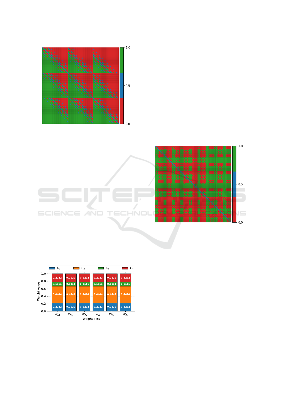
Figure 1: Identified MEJ matrix.
There is, however, a way to determine global
weights based on the characteristic objects (Wi˛eck-
owski et al., 2023a). With the information about
characteristic objects and their preferences calculated
based on the MEJ, we can fit the linear regression in
order to obtain the global criteria weights from the
model.
Identified global weights W
LR
are presented in
Figure 2. Other bars present local weights for each
alternative identified using the algorithm described
previously in Section 2.5. Local weights are trying
to answer the question of how specific criteria influ-
ence the evaluation of the specific alternative. In the
case of the linear model, the global weights are identi-
fied using linear regression, and the local weights are
equal. The criterion that influences the preference val-
ues most is the C
2
. Then criteria C
1
and C
4
have the
same weights and, therefore, are in a tie, and crite-
rion C
3
has a smaller influence on the final preference
value. The equality of the global and local weights
suggests that the preference values of the alternatives
change linearly if we linearly change the criteria val-
ues.
Figure 2: Visualization of the identified weights.
3.2 Example with the ESP-COMET
Model
In this example, to simulate non-linear expert prefer-
ences, we use a recently proposed ESP-COMET al-
gorithm (Shekhovtsov et al., 2023) described fully in
Section 2.2. For the same characteristic values as pre-
sented in the linear example, we randomly choose the
ESP value:
ESP = {0.3371,0.5218, 0.9290, 0.5265},
and identified the model according to it.
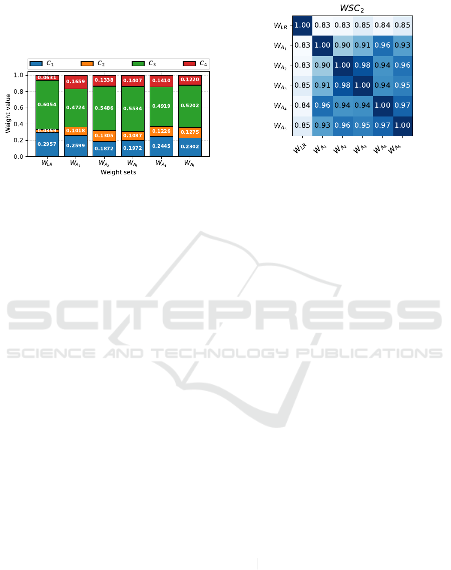
Figure 3 presents the resulting MEJ matrix. As
we can see, there are more ties in this matrix, and the
pattern is less repeatable than in the MEJ presented
in Figure 1. This implies that the identified model is
non-linear in this case.
Figure 3: MEJ matrix identified using ESP-COMET algo-
rithm.
We calculate the preferences of the characteris-
tic objects based on the identified MEJ matrix and
evaluate alternatives presented in Table 1 using the
COMET method. The preference vector for this ex-
ample is defined as:
P
(ESP)
= {0.7614,0.2488,0.1996,0.1890, 0.6230},
The bigger value P
i
indicates that alternative A
i
is better. Following this rule, we can determine the
ranking of the alternatives, which differs from the or-
der obtained with linear expert function: A
1
> A
5
>
A
2
> A
3
> A
4
. Next, we process the obtained COMET
model as well as the alternatives using the algorithm
of identification of the global weights using the lin-
ear regression, as well as the described in Section 2.5
algorithm for the local weights identification.
The results of the weights identification are visual-
ized in Figure 4. As we can see, the weight vectors are
quite different. In the case of the complex non-linear
ICAART 2024 - 16th International Conference on Agents and Artificial Intelligence
474

decision function, the final preference value may be
changed differently for different alternatives, creating
differences in the local weights for investigated alter-
natives.
Figure 4: Visualization of the identified weights.
Analyzing Figure 4 we can see that the identi-
fied weights vary significantly. The identified global
weight for the criterion C
1
is 0.2957; however, the
importance of this criterion in the different alterna-
tives’ evaluation changes from 0.1872 for the alterna-
tive A
2
to 0.2599 for the alternative A
1
. The global
weight for the C
2
is 0.0359, but for alternatives, it
varies from 0.1018 to 0.1305, which is significantly
bigger. Next, the local weights for the criterion C
3
change from 0.4724 to 0.5534. However, the identi-
fied global weight is 0.6054. For the last criterion C
4
,
the global weight is 0.0631, and the local weights are
changed from 0.1220 to 0.1659. Those differences
show that the global weights are not necessarily the
same as local weights for the alternatives in the spe-
cific decision problem.
Next, we calculate the W SC
2
coefficient between
every pair of the identified weights and present it in
the form of a heatmap in Figure 5. The range of the
W SC
2
values is [0,1], where 1 means equal weights
and 0 most different weights. As we can see, the val-
ues in the heatmap suggest that the identified weights
are rather similar. The lower W SC
2
value calculated
between local weights for alternatives A
2
and A
4
is
equal to 0.65. The most similar pair of the weights
is local weights for alternatives A
1
and A
5
, and the
W SC
2
coefficient value is equal to 0.94 for this com-
parison. The identified global weights are most sim-
ilar to the local weights identified for the alternatives
A
1
(0.93) and A
5
(0.92).
3.3 Simulation on Local Weights
In this section, we describe the simulation designed
to investigate the differences between global weights
computed based on a COMET model identified based
on random ESP and local weights identified with the
Figure 5: Similarities between weights calculated using
W SC
2
.
algorithm described in Section 2. To help understand
the simulation, we illustrate it with the use of Algo-
rithm 2. This algorithm describes the single simu-
lation run. At first, we should define the number of
alternatives and the number of criteria to generate.
Next, the procedure creates a random matrix A with
size n×r and a random ESP vector based on the num-
ber of criteria r. Random values are drawn from the
uniform distribution with range [0,1). The COMET
method is designed in such a way that it does not re-
quire a normalization, therefore these simulation re-
sults can also be generalized for other ranges of the
data. Next, we need to define the ESP Expert object
based on ESP. We will evaluate characteristic objects
based on them. We also need to create a cvalues struc-
ture which defines a grid of the characteristic objects
based on ESP, as it was described in (Shekhovtsov
et al., 2023). Next, we determine local weights lw
i
for each alternative A
i
and global weights gl utiliz-
ing a linear regression model as described in (Wi˛eck-
owski et al., 2023a). These results returned from the
simulation procedure and were processed later.
Data: Number of alternatives n
Data: Number of criteria r
1 A ← random_matrix(n, r);
2 ESP ← random_esp(r);
3 expert ← ESPExpert(ESP);
4 cvalues ← expert.make_cvalues();
5 comet ← COMET(cvalues, expert);
6 lw ← empty_array();
7 for i in {1,2,. . .,n} do
8 lw
i
← get_local_weights(comet, A
i
);
9 end
10 gl ← get_global_weights(comet);
11 return gl,lw
Algorithm 2: Single iteration of the simulation.
Comparing Global and Local Weights in Multi-Criteria Decision-Making: A COMET-Based Approach
475

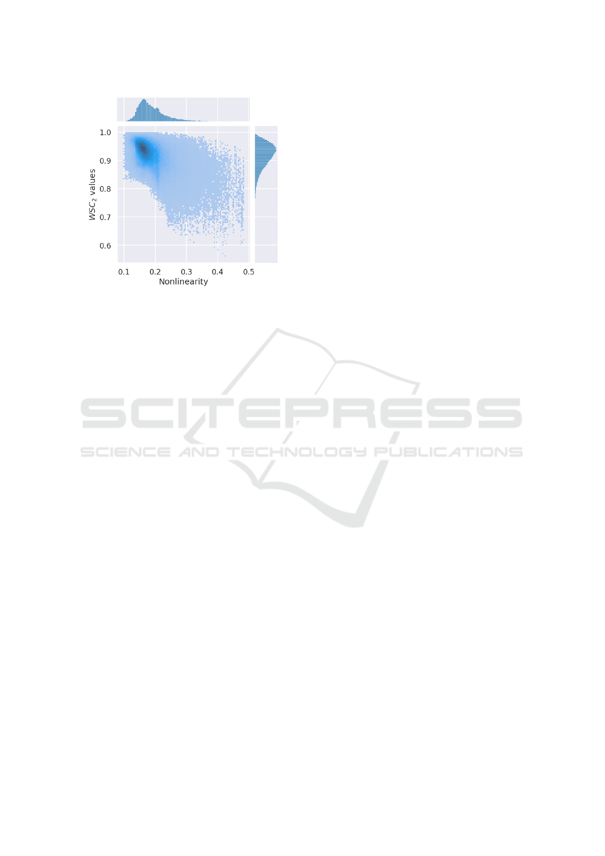
Figure 6: Results of the simulations computed based on
50,000 runs.
We ran the simulation procedure 50,000 times for
the number of criteria r = 4 and the number of alter-
natives n = 5. Such numbers were chosen because it
is more realistic to be able to identify the MEJ matrix
for this size of the decision problem. However, we
also ran the simulations for other values r and n and
got very similar results. Based on gl and lw vectors
collected during the simulation, we compute nonlin-
earity index values as well as W SC
2
values to get a nu-
merical representation of the differences in the local
and global weights. Notice that because one gl vec-
tor is related to n = 5 lw vectors, nonlinearity index
values were duplicated to correspond to each W SC
2
value calculated between gl and each lw
i
vector from
one simulation run.
Figure 6 contains the visualization of the joint dis-
tribution of both the nonlinearity index and W SC
2
variables. On the side parts of the visualization, we
can also see the respective distributions of these two
variables. The mean WSC
2
value is 0.91, and the av-
erage nonlinearity index value is 0.19. It can be seen
as the darkest point in the visualization. Also, it can
be seen that the resulting W SC
2
values are laid in the
range [0.5,1.0], and nonlinearity index values lie in
the range [0.1,0.5]. The Pearson r correlation value
computed on both variables equals −0.52, which im-
plies that there is a small level of reversed correlation
between these variables. It also can be observed in
the visualization, where smaller values of the nonlin-
earity index frequently correspond to higher values of
W SC
2
. For the higher value of the nonlinearity index,
it is almost impossible for global and local weights to
match, and in those cases, most of the W SC
2
values
are below 0.9.
The observations drawn from the simulation and
its results demonstrate how important local weights
can be for deeper analysis of the decision problems,
especially when it was solved with the help of expert
knowledge. If the model identified by an expert is
nonlinear, we cannot simply draw the global weights
and use them to evaluate alternatives further. The
local weights computed for the identified decision
model can be crucial in further analysis, as they can
answer the question of what should be improved on
the existing alternatives to be evaluated higher in the
decision problem. This information can also be used
when looking for better decision alternatives than the
ones included in the consideration.
4 CONCLUSION
In this paper, we demonstrate two simple examples
of local weights identification for the alternatives in
decision-making problems. Additionally, we design
the simulation experiment based on the second exam-
ple, which demonstrates the importance of the local
weights in an in-depth analysis of the decision prob-
lem. The utilized approach is based on the Character-
istic Objects Method and demonstrates its efficiency
in the identification of the local weights in both lin-
ear and nonlinear decision problems. To simulate the
artificial expert in the simulation, we used the ESP-
COMET model, which can simulate the identification
of the MEJ matrix based on a randomly chosen ESP.
The presented experiments show that in the case of the
linear problem, the global criteria weights identified
from the evaluated characteristic objects using linear
regression are equal to the local weights. However,
in the case of complex nonlinear problems, the W SC
2
similarity value between local and global weights can
fall below 0.6.
This demonstrates the importance of identifying
local weights for the deeper decision problem analy-
sis. For example, identified local weights can answer
how much different criteria influence the final evalua-
tion of the specific alternatives. It can also be helpful
to have an idea of how the alternatives in the consid-
ered set can be improved to score higher preference
values.
Future research may include further investigation
of the properties of local weights in the context of the
practical decision-making problem. We also want to
improve the conception of the local weights and look
for ways to determine them more precisely.
ICAART 2024 - 16th International Conference on Agents and Artificial Intelligence
476

REFERENCES
Biswas, S., Bandyopadhyay, G., Pamucar, D., and Sanyal,
A. (2022). A decision making framework for com-
paring sales and operational performance of firms
in emerging market. International Journal of
Knowledge-based and Intelligent Engineering Sys-
tems, 26(3):229–248.
Choo, E. U., Schoner, B., and Wedley, W. C. (1999). In-
terpretation of criteria weights in multicriteria deci-
sion making. Computers & Industrial Engineering,
37(3):527–541.
Dezert, J., Tchamova, A., Han, D., and Tacnet, J.-M.
(2020). The spotis rank reversal free method for multi-
criteria decision-making support. In 2020 IEEE 23rd
International Conference on Information Fusion (FU-
SION), pages 1–8. IEEE.
Elanchezhian, C., Ramnath, B. V., and Kesavan, R. (2010).
Vendor evaluation using multi criteria decision mak-
ing. International Journal of Computer Applications,
5(9):4–9.
Faizi, S., Rashid, T., Sałabun, W., Zafar, S., and W ˛atrób-
ski, J. (2018). Decision making with uncertainty us-
ing hesitant fuzzy sets. International Journal of Fuzzy
Systems, 20:93–103.
Faizi, S., Sałabun, W., Rashid, T., W ˛atróbski, J., and Zafar,
S. (2017). Group decision-making for hesitant fuzzy
sets based on characteristic objects method. Symme-
try, 9(8):136.
Habeeb, R., Hussain, I., Al-Ansari, N., and Sammen, S. S.
(2022). A proposed comparative algorithm for re-
gional crop yield assessment: An application of char-
acteristic objects method. Mathematical Problems in
Engineering, 2022.
Jahan, A. and Edwards, K. (2013). Vikor method for ma-
terial selection problems with interval numbers and
target-based criteria. Materials & Design, 47:759–
765.
Kizielewicz, B., Shekhovtsov, A., and Sałabun, W. (2021).
A new approach to eliminate rank reversal in the mcda
problems. In Computational Science–ICCS 2021:
21st International Conference, Krakow, Poland, June
16–18, 2021, Proceedings, Part I, pages 338–351.
Springer.
Kizielewicz, B., Shekhovtsov, A., and Sałabun, W.
(2023). pymcdm—the universal library for solving
multi-criteria decision-making problems. SoftwareX,
22:101368.
Kizielewicz, B., W ˛atróbski, J., and Sałabun, W. (2020).
Identification of relevant criteria set in the mcda
process—wind farm location case study. Energies,
13(24):6548.
Kozlov, V. and Norek, T. (2021). Towards objective multi-
criteria drone evaluation based on vikor and comet
methods. Procedia Computer Science, 192:4522–
4531.
Lipka, W. and Szwed, C. (2021). Multi-attribute rating
method for selecting a clean coal energy generation
technology. Energies, 14(21):7228.
Mahmoody Vanolya, N. and Jelokhani-Niaraki, M. (2021).
The use of subjective–objective weights in gis-based
multi-criteria decision analysis for flood hazard as-
sessment: A case study in mazandaran, iran. Geo-
Journal, 86:379–398.
Manolitzas, P., Grigoroudis, E., Christodoulou, J., and Mat-
satsinis, N. (2020). S-meduta: Combining balanced
scorecard with simulation and mcda techniques for the
evaluation of the strategic performance of an emer-
gency department. In GeNeDis 2018: Computational
Biology and Bioinformatics, pages 1–22. Springer.
Saaty, T. L. (2004). Decision making—the analytic hier-
archy and network processes (ahp/anp). Journal of
systems science and systems engineering, 13:1–35.
Sałabun, W. (2015). The characteristic objects method:
a new distance-based approach to multicriteria
decision-making problems. Journal of Multi-Criteria
Decision Analysis, 22(1-2):37–50.
Shekhovtsov, A. (2023). Evaluating the performance
of subjective weighting methods for multi-criteria
decision-making using a novel weights similarity co-
efficient. Procedia Computer Science, 225:4785–
4794.
Shekhovtsov, A., Kizielewicz, B., and Sałabun, W. (2023).
Advancing individual decision-making: An extension
of the characteristic objects method using expected so-
lution point. Information Sciences, 647:119456.
Ullah, K., Hamid, S., Mirza, F. M., and Shakoor, U. (2018).
Prioritizing the gaseous alternatives for the road trans-
port sector of pakistan: A multi criteria decision mak-
ing analysis. Energy, 165:1072–1084.
Wi˛eckowski, J. and Dobryakova, L. (2021). A fuzzy as-
sessment model for freestyle swimmers-a comparative
analysis of the mcda methods. Procedia Computer
Science, 192:4148–4157.
Wi˛eckowski, J., Kizielewicz, B., Paradowski, B.,
Shekhovtsov, A., and Sałabun, W. (2023a). Ap-
plication of multi-criteria decision analysis to identify
global and local importance weights of decision crite-
ria. International Journal of Information Technology
& Decision Making, 22(06):1867–1892.
Wi˛eckowski, J., Kizielewicz, B., Shekhovtsov, A., and
Sałabun, W. (2023b). Rancom: A novel approach to
identifying criteria relevance based on inaccuracy ex-
pert judgments. Engineering Applications of Artificial
Intelligence, 122:106114.
Yang, C. and Qian, Z. (2023). Street network or functional
attractors? capturing pedestrian movement patterns
and urban form with the integration of space syntax
and mcda. URBAN DESIGN International, 28(1):3–
18.
Yombi, J. C., De Greef, J., Marsin, A.-S., Simon, A.,
Rodriguez-Villalobos, H., Penaloza, A., and Belkhir,
L. (2020). Symptom-based screening for covid-19 in
healthcare workers: the importance of fever. The Jour-
nal of hospital infection, 105(3):428.
Comparing Global and Local Weights in Multi-Criteria Decision-Making: A COMET-Based Approach
477