Using the Polynomial Particle-in-Cell Method for Liquid-Fabric

Interaction

Robert Dennison and Steve Maddock

The University of Shefﬁeld, U.K.

ﬁ

Keywords:

Physically-Based Modeling, Fluid Simulation, Cloth Simulation.

Abstract:

Liquid-fabric interaction simulations using particle-in-cell (PIC) based models have been used to simulate a

wide variety of phenomena and yield impressive visual results. However, these models suffer from numerical

damping due to the data interpolation between the particles and grid. Our paper addresses this by using the

polynomial PIC (PolyPIC) model instead of the afﬁne PIC (APIC) model that is used in current state-of-the-

art wet cloth models. Theoretically, PolyPIC has lossless energy transfer and so should avoid any problems

of undesirable damping and numerical viscosity. Our results show that PolyPIC does enable more dynamic

coupled simulations. The use of PolyPIC allows for simulations with reduced numerical dissipation and

improved resolution of vorticial details over previous work. For smaller scale simulations, there is minimal

impact on computational performance when using PolyPIC instead of APIC. However, as simulations involve

a larger number of particles and mesh elements, PolyPIC can require up to a 2.5× as long to generate 4.0s of

simulation due to a requirement for a decrease in timestep size to remain stable.

1 INTRODUCTION

In physics-based simulations for computer graphics,

increasing attention is being focused on simulations

involving a combination of two or more physical me-

dia. One area of particular interest is simulating the

complex interactions between ﬂuid and porous fabric.

The liquid-fabric interaction model of Fei et al (Fei

et al., 2018) is widely considered as the state-of-the-

art for this kind of coupled simulation. They make use

of the afﬁne particle-in-cell (APIC) model for the ﬂu-

ids and the material point method (MPM) using APIC

transfers for cloth and yarn objects.

Particle-in-cell (PIC) methods are a class of hybrid

Eulerian-Lagrangian simulation methods, designed to

beneﬁt from the ease of particle advection found in

Lagrangian methods with the simplicity of calculat-

ing forces and material properties on a regular Eule-

rian grid. In each time step, particle information is

interpolated to nearby grid nodes where an updated

velocity can be calculated. This new velocity can then

be interpolated back to the particles which can be ad-

vected through the simulation domain. A known issue

with PIC methods is that they suffer from numerical

dissipation, as the interpolation stages act as a ﬁlter of

high frequency and rotational velocities. This means

that ﬂuid simulations using PIC methods can seem

overly viscous. APIC was introduced as an improve-

ment to the standard PIC model (Jiang et al., 2015)

and was developed to reduce the numerical dissipa-

tion by considering rotational velocity. Since its in-

troduction, APIC has seen wide adoption by the vi-

sual effects industry.

While APIC was developed in an effort to reduce

damping of rotational velocities, it has been shown to

still be introduce numerical damping. This makes it

more challenging to use real world values for viscos-

ity and elasticity, as the model will introduce viscosity

numerically. The polynomial particle-in-cell model

(PolyPIC) was introduced as a generalised extension

of APIC to further reduce numerical dissipation (Fu

et al., 2017), and has been shown to theoretically be

able to achieve lossless energy transfers during the in-

terpolation stages. By using a method with reduced

energy loss, real world empirical data can be used as

the model parameters, allowing for easier recreation

of real world scenes by artists.

Our paper is the ﬁrst to use PolyPIC for liquid-

fabric interactions. We improve the work of Fei et

al by incorporating polynomial transfers between the

particles and grid. By substituting the afﬁne trans-

fers of APIC for higher order polynomials, the nu-

merical damping of the model can be reduced. This

also requires an alteration of some aspects of the pre-

244

Dennison, R. and Maddock, S.

Using the Polynomial Particle-in-Cell Method for Liquid-Fabric Interaction.

DOI: 10.5220/0012359300003660

Paper published under CC license (CC BY-NC-ND 4.0)

In Proceedings of the 19th International Joint Conference on Computer Vision, Imaging and Computer Graphics Theory and Applications (VISIGRAPP 2024) - Volume 1: GRAPP, HUCAPP

and IVAPP, pages 244-251

ISBN: 978-989-758-679-8; ISSN: 2184-4321

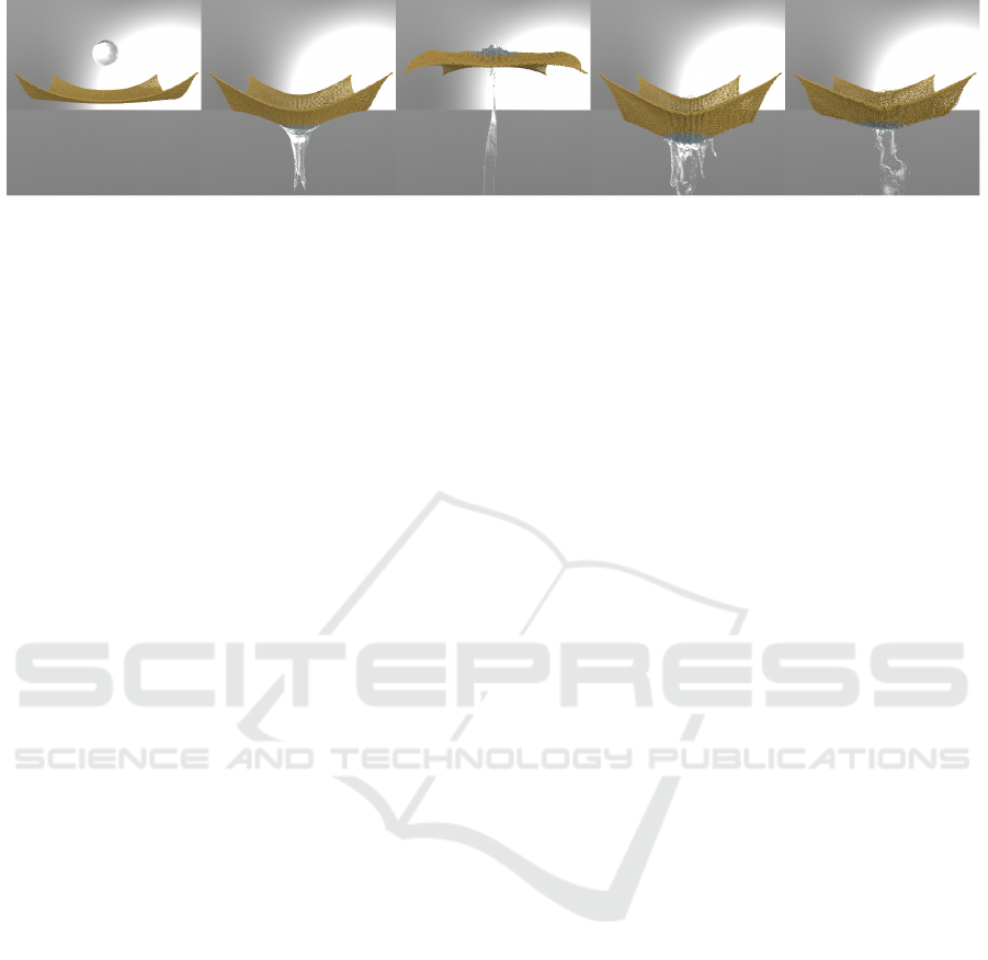
Figure 1: Fluid splashing onto a square of yarn fabric using PolyPIC transfers.

sented PolyPIC method to improve simulation stabil-

ity. The results give a comparison of PolyPIC with

APIC for coupled simulation scenarios and demon-

strate that PolyPIC provides improved preservation of

rotational velocity, leading to more dynamic simula-

tions. The presented scenarios give a comparison of

APIC and PolyPIC in a pure ﬂuid simulation to show-

case the differences of the two simulation approaches.

The remainder of this paper is structured into ﬁve

sections. Section 2 describes related work. Sec-

tion 3 explains the implementation of PolyPIC for the

liquid-fabric simulation. The results in section 4 pro-

vide a comparison of PolyPIC and APIC, with a dis-

cussion in section 5. Section 6 presents conclusions.

2 RELATED WORK

Early work on wet cloth models focused on non-

porous thin shells interacting with ﬂuids (e.g. (Harada

et al., 2007)), with subsequent work involving porous

volumes (Lenaerts et al., 2008). The main drawback

of this work was that it used a smoothed particle hy-

drodynamics framework, thus requiring a large num-

ber of particles internal to the object’s volume and

impacting on computational performance. Huber et

al (Huber et al., 2011) improved the computational

performance by using a cellular automata approach

which allowed for simple parallelization. Patkar et

al (Patkar and Chaudhuri, 2013) used a mesh-based

approach for solid simulation to remove the need for

simulating large numbers of solid particles and also

incorporated additional ﬂuid effects such as dripping

and surface ﬂow.

Further developments came with the application

of position based dynamics (M

uller et al., 2007) to

the model presented by Lenaerts et al, thus allowing

for larger time steps to be used (Shao et al., 2018).

Another recent development by Fei et al (Fei et al.,

2018) demonstrates both a porous cloth model using

discrete shells (Grinspun et al., 2003) and discrete

rods (Bergou et al., 2008) discretized using the ma-

terial point method (MPM) (Sulsky et al., 1994) for

cloth and yarn simulations, respectively. Zheng et al

then added further realism to liquid-yarn interactions

by modelling the defects in the constituent ﬁbres of a

material (Zheng et al., 2021). However, this work has

currently only been used to model static fabric.

Particle-in-cell methods have seen extensive use

since ﬁrst being introduced by Harlow et al (Har-

low, 1962). The severe numerical dissipation of this

method due to ﬁltering caused by the number of inter-

polation steps led to the development of the ﬂuid im-

plicit particle (FLIP) method, which bypassed some

of the interpolation steps to increase the dynamism of

simulations by interpolating only the change in veloc-

ity from the grid to the particles rather than interpo-

lating the velocity (Brackbill and Ruppel, 1986). The

major drawback of the FLIP method was that reduced

dissipation came at the cost of introducing more noise

and instability to the simulations.

Jiang et al (Jiang et al., 2015) developed the APIC

method as a way of reducing the numerical dissipation

of PIC in a stable way by storing an afﬁne transform

matrix on each particle, as well as a velocity vector.

This reduced the energy loss of the PIC method and

improved the stability of FLIP, and also improved the

preservation of angular momentum of both previous

iterations of the model. Recently PolyPIC (Fu et al.,

2017) was developed as a generalized extension of

APIC to allow for higher order transfers during the

grid/particle transfers, further reducing the numeri-

cal dissipation and improving preservation of angular

momentum. It achieves this by replacing the afﬁne

matrix used to store information about angular mo-

mentum with a more general polynomial function.

The popularity of PIC methods led to their appli-

cation to deformable materials by Sulsky et al to cre-

ate MPM (Sulsky et al., 1994). Subsequent PIC de-

velopments have also continued to be adapted to elas-

tic solids to continually improve MPM simulations,

and MPM has been successfully applied to simulate

a wide variety of materials such as snow (Stomakhin

et al., 2013), viscoelastic solids (Fang et al., 2019)

and even materials with phase changes such as lava

or butter (Stomakhin et al., 2014). Despite the im-

provements of PolyPIC over APIC, PolyPIC has not

yet been adapted to coupled simulation scenarios.

Using the Polynomial Particle-in-Cell Method for Liquid-Fabric Interaction

245

3 METHOD

This paper builds on the work of Fei et al by replacing

the APIC model with the PolyPIC model. APIC and

PolyPIC differ only in the transfer steps (as shown in

Figure 2), meaning PolyPIC transfers can be substi-

tuted into the model in the place of APIC transfers.

Section 3.1 presents the standard PIC model, section

3.2 describes how APIC builds upon this and PolyPIC

is explained in section 3.3. Finally, section 3.4 de-

scribes the application of PolyPIC to a mixture model.

Fei et al used a staggered marker-and-cell (MAC) grid

approach as it provides more accurate central differ-

ences over a standard collocated grid approach, so all

work presented here is applied to MAC grids.

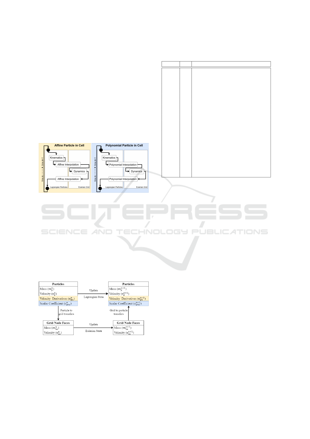
Figure 2: The difference between the APIC and PolyPIC

algorithms is the method of transferring data between the

particles and the grid. PolyPIC uses generalized higher or-

der polynomials whereas APIC uses afﬁne transformation

matrices. (Based on Figure 7 in (Jiang et al., 2015)).

3.1 The Particle-in-Cell Method

The standard PIC model consists of particles which

store information about their mass and velocity,

which is interpolated to/from the grid node faces to

advect the particles around the simulation domain, as

shown in Figure 3. The yellow and blue boxes will be

considered in subsections 3.2 and 3.3, respectively.

Figure 3: The data stored by particles and grid node faces in

PIC methods. White background boxes are consistent be-

tween all PIC variants. Velocity derivatives (yellow back-

ground) are introduced for APIC and scalar coefﬁcients

(blue boxes) are introduced in PolyPIC. (Based on a dia-

gram in (Fu et al., 2017)).

Table 1: Notation used throughout this paper. Values are of

type scalar s, vector v or matrix m.

Notation Type Meaning

∆t s size of time step

∆x s size of grid node

v position of particle p

iα

v position of face α of grid node i

s mass of particle p

v velocity of particle p

iα

s mass of face α of grid node i

iα

v velocity of face α of grid node i

˜v

iα

v intermediate velocity of face α of grid node i

ipα

s contribution of particle p to face α of grid node i

ipα

s mass contributed by particle p to face α of grid

node i

(mv)

ipα

v momentum contributed by particle p to face α of

grid node i

m velocity derivatives of particle p, as described in

(Jiang et al., 2015)

pα

v velocity derivatives used for MAC grids

prα

s scalar coefﬁcient of scalar mode r for particle p in

axis α

I m identity matrix

v basis vector for axis α

A PIC simulation consists of a total of P particles

and N

grid nodes, where superscript n is used for a

given quantity at the current timestep n (e.g. v

is the

velocity of particle p at timestep n) and α represents

a face of a grid node for each axis 1 ≤ α ≤ d, where

d is the number of dimensions. The notation used

throughout this paper is summarised in Table 1.

In the standard PIC method, each particle stores

its own mass and velocity. A weight function N(x)

is deﬁned to calculate the contribution of a particle

to nearby grid cells during the interpolation steps and

vice versa. Each particle within a nearby region of a

grid node contributes some of its mass to each face

(Equation 1). The mass contribution of each parti-

cle can then be multiplied by the particle’s velocity to

calculate the momentum contribution of each particle

(Equation 2). The momentum contribution can then

be summed over all particles to calculate the total mo-

mentum for the grid node face (Equation 3). The total

mass of the grid node face is the mass contributions

of all particles (Equation 4). Finally, the velocity of

each grid node face can be calculated by dividing the

momentum by the mass (Equation 5).

ipα

= m

ipα

(1)

(mv)

ipα

= m

ipα

(2)

(mv)

iα

∑

p=0

(mv)

ipα

(3)

iα

∑

p=0

ipα

(4)

iα

= (mv)

iα

(5)

GRAPP 2024 - 19th International Conference on Computer Graphics Theory and Applications

246

where w

ipα

= N(x

pα

− x

iα

) is the contribution of par-

ticle p to face α of grid node i.

The mass of a grid node can change throughout

the simulation, but the masses of particles are ﬁxed.

This means when interpolating from the grid nodes

to the particles, we only update the particles’ veloci-

ties. Once the intermediate grid velocities ˜v

iα

n+1

have

been calculated, they are interpolated back to the par-

ticles. To calculate the contribution of grid node mo-

mentum to each particle, ﬁrst the momentum of each

grid node must be calculated. This is done by mul-

tiplying the mass of each node face by the interme-

diate velocity of each node face and summing over

the number of faces (Equation 6). Then the momen-

tum of each particle can be calculated by summing

the contributed momentum of each grid node over the

number of grid nodes (Equation 7). Finally, the ve-

locity of each particle can be calculated by dividing

the momentum by the particle mass (Equation 8).

(mv)

n+1

∑

α=1

ipα

˜v

iα

n+1

(6)

(mv)

n+1

∑

i=0

(mv)

n+1

(7)

n+1

= (mv)

n+1

(8)

3.2 The Afﬁne PIC Method

In the APIC method, alongside mass and velocity

each particle also stores an afﬁne matrix of velocity

derivatives to enhance the preservation of rotational

velocities (see Figure 3). Equations 1 and 4, used for

transferring mass from the particles to the grid nodes,

remain unchanged for APIC. The updated momentum

transfer takes into account the velocity derivatives to

preserve angular momentum (Equation 9 (Equation

13 in Jiang et al)). The grid momentum can calcu-

lated as with PIC using Equation 3.

(mv)

ipα

= m

ipα

+ c

pα

− x

iα

)) (9)

where m

ipα

is calculated using Equation 1.

The momentum transfers from the grid nodes to

the particles are the same as those used in the standard

PIC method given by Equations 6 - 8. At this stage

the velocity derivatives of a particle, c

pα

, are updated

by calculating the gradient of the weights relating that

particle to the grid node faces, ∇w

ipα

, multiplied by

the intermediate velocity, then summing over all grid

nodes (Equation 10 (Equation 14 in Jiang et al)).

n+1

pα

∑

∇w

ipα

˜v

iα

n+1

(10)

3.3 The Polynomial PIC Method

PolyPIC replaces the afﬁne matrix of APIC with gen-

eralized polynomials which allow for a wider range of

local behaviour capture (see Figure 3). For PolyPIC

the number of modes used is given by N

. It uses

polynomials of the form:

s(z) =

∏

β=1

(11)

where z

is the β

component of z ∈ R

with i

∈ Z

Before deﬁning the transfers, we must ﬁrst deﬁne

a map of the simulation conﬁguration at time t

n+1

, denoted as ξ

n+1

(x). As described by Fu et al, this

map can take different forms for constant or afﬁne

material motion. Here, the afﬁne map is given by

Equation 12 (Equation 10 in Fu et al).

n+1

(x) = x

+ (I + ∆tC

n+1

)

−1

(x − x

n+1

) (12)

The method of calculating C

is given in detail

in (Jiang et al., 2015). The momentum transfer from

the particles to the grid is then calculated by taking

the sum of all the scalar modes multiplied by the cor-

responding scalar coefﬁcients, given by Equation 13

(Equation 11 in Fu et al). The momentum contribu-

tion of each particle to the grid node faces can then be

summed over all particles (Equation 3). The veloc-

ity of each grid node face can then be calculated by

dividing the momentum by the mass (Equation 5).

(mv)

ipα

= m

ipα

∑

r=0

(ξ

iα

− x

n−1

prα

(13)

where s

is scalar mode r. The coefﬁcients c

prα

are

calculated as a minimisation problem as described by

Fu et al. To efﬁciently calculate the coefﬁcients, the

resultant linear system requires each dimension to be

decoupled. The coefﬁcients for modes 1 ≤ r ≤ 2

are

naturally mass-orthogonal and so solutions can be ef-

ﬁciently found. However, higher order coefﬁcients

< r ≤ N

require modiﬁcation to be orthogonal-

ized. This is achieved by substituting the quadratic

terms, z

, in Equation 11 with g

) deﬁned in Equa-

tion 14. In contrast to the equation presented in Fu et

al, the variables in Equation 14 are modiﬁed to or-

thogonalize the matrix, which produces more stable

simulations.

) = (w

)

− w

(∆x

− 4z

)

∆x

−

∆x

(14)

Again, the momentum transfers from the grid to

the particles are the same as those used in the stan-

dard PIC method given by Equations 6, 7 and 8. At

Using the Polynomial Particle-in-Cell Method for Liquid-Fabric Interaction

247

this stage, the velocity derivatives C

can be calcu-

lated using the method described by Jiang et al and

the coefﬁcients c

prα

can be calculated as described by

Fu et al.

3.4 Liquid-Fabric Interaction

The model presented by Fei et al relies on the use of

mixture theory to simulate the interactions between

ﬂuid and cloth (Nielsen and Østerby, 2013). There-

fore, the momentum transfers need to be altered in

order to be applied to mixtures. Let m

s,p

be the mass

of a solid particle p at time n and m

f ,p

be the mass

of a ﬂuid particle p at time n. The ﬂuid transfers are

then the same as those given in Equations 3, 5 and 13,

except only particles tagged as ﬂuids are considered

(Equations 15 - 17).

)

ipα

= m

f ,ipα

∑

r=0

(ξ

iα

− x

n−1

prα

(15)

)

iα

∑

)

ipα

(16)

f ,iα

= (m

)

iα

f ,iα

(17)

The solid transfers are very similar to the ﬂuid

transfers, except that absorbed ﬂuid particles must

be considered. To take account of absorption, we

must also consider the mass of absorbed ﬂuid par-

ticles when transferring the momentum of solids to

the grid. The total mass of a solid particle is there-

fore given by summing the mass of the solid parti-

cle itself and the mass of the absorbed ﬂuid particle,

s,ipα

+ m

f ,ipα

). These solid-ﬂuid mixture momen-

tum transfers are given in Equations 18 - 20.

)

ipα

= (m

s,ipα

+ m

f ,ipα

)

∑

r=0

(ξ

iα

− x

n−1

prα

(18)

)

iα

∑

)

ipα

(19)

s,iα

= (m

)

iα

/(m

s,ipα

+ m

f ,ipα

) (20)

4 RESULTS

Four scenarios have been used to test the model that

has been developed:

• Figure 4 shows a simple dam break scenario to

highlight the differences between APIC ﬂuids and

PolyPIC ﬂuids.

• Figure 5 shows a ball of ﬂuid falling onto a small

square of cloth draped over a sphere.

• Figure 6 shows a ball of ﬂuid falling onto a small

square of yarn-based fabric draped over a sphere.

• Figure 7 is similar to the small yarn scenario but

shows a larger volume of liquid falling onto a

medium sized square of yarn-based fabric.

The latter three scenarios were used by Fei et al,

enabling a comparison of the original model using

APIC and the new model using PolyPIC. In the sim-

ulation results, particle colours are based on current

particle velocity, where dark blue represents a low ve-

locity and red a high velocity. Videos of each simula-

tion can be found in the supplementary video.

The simple dam break scenario (Figure 4) high-

lights the difference between PolyPIC and APIC out-

side of a coupled simulation context. This shows that

using PolyPIC increases the conservation of angular

momentum and so improves the resolution of vorticial

detail of the ﬂuid. As the ﬁnal frame shows, PolyPIC

particles have higher velocities than in APIC show-

ing that numerical damping is reduced when using

PolyPIC.

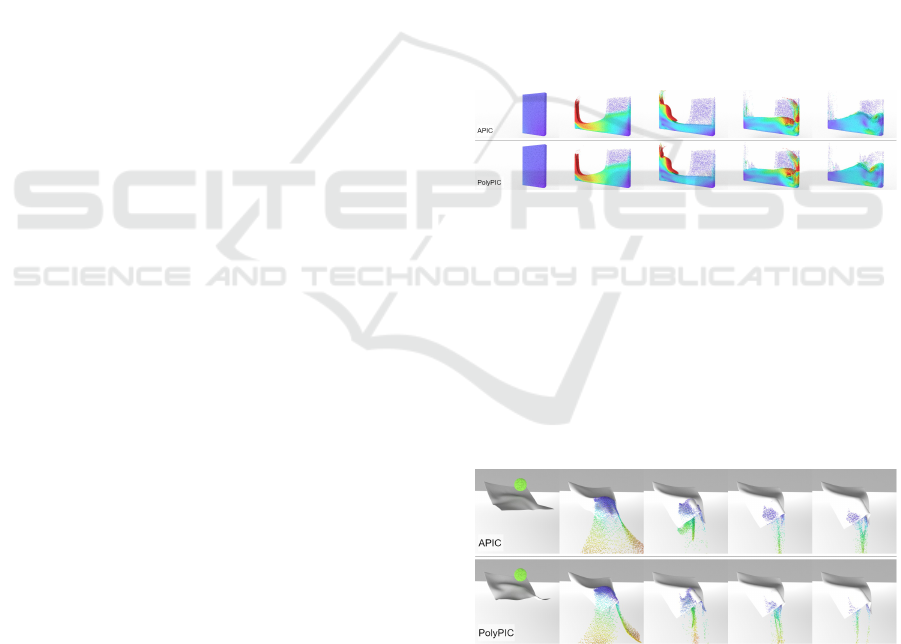
Figure 4: A small dam break scenario using APIC (top) and

PolyPIC (bottom) transfers. Particle colours indicate veloc-

ity (dark blue = low, red = high). PolyPIC shows improved

resolution of vorticial details.

A ball of ﬂuid falling onto a small square of cloth

fabric is shown in Figure 5. This example demon-

strates the reduced numerical damping of PolyPIC

causes less of the ﬂuid to be absorbed by the cloth,

as more splashes off as it is falling. The ﬂuid that

is absorbed exhibits more thin strand behaviour as it

drips from the cloth in PolyPIC than APIC.

Figure 5: Fluid splash onto a small piece of cloth using

APIC (top) and PolyPIC (bottom) transfers. Particle colours

indicate velocity (dark blue = low, red = high). The reduced

damping means that more ﬂuid splashes off the piece of

cloth rather than being absorbed. The ﬂuid that is absorbed

exhibits more thin strand behaviour as it drips from the cloth

in PolyPIC than APIC (see frame 4).

GRAPP 2024 - 19th International Conference on Computer Graphics Theory and Applications

248

A ball of ﬂuid falling onto a small square of yarn

fabric is shown in Figure 6. This scenario shows that

the PolyPIC yarns exhibit less sagging than APIC, as

they stretch less under their own weight. The reduced

damping also makes the PolyPIC yarns spring back

from being stretched by the ﬂuid faster.

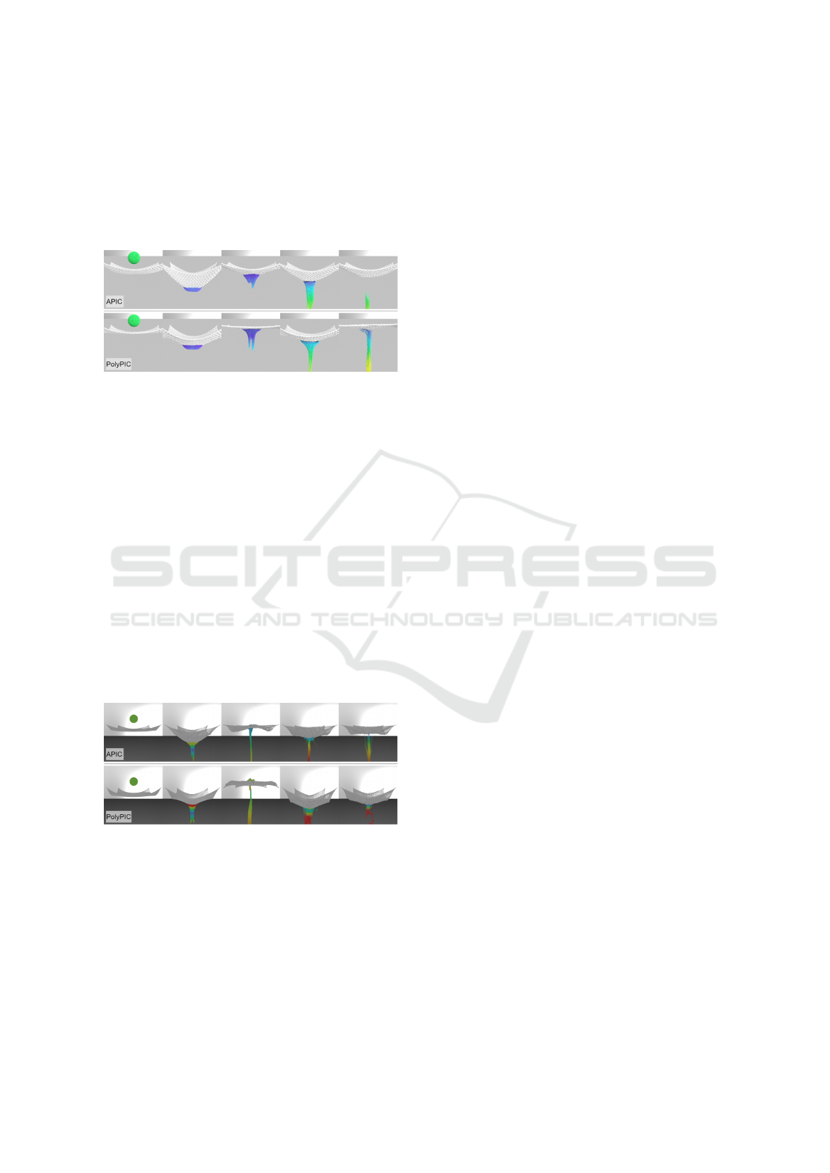
Figure 6: Fluid splashing onto a small square of yarn fabric

using APIC (top) and PolyPIC (bottom) transfers. Particle

colours indicate velocity (dark blue = low, red = high). The

PolyPIC yarns exhibit less sagging than APIC (see frame

1). The reduced damping makes the PolyPIC yarns spring

back faster from being stretched (see frames 3-5).

Finally, a ball of ﬂuid falling onto a medium

square of yarn fabric is shown in Figure 7. This ex-

ample demonstrates that PolyPIC increases the trans-

fer of energy from the falling ﬂuid to the suspended

yarn. Due to issues with collision detection and res-

olution, this increased transfer of energy causes the

yarns to become more tangled than when using APIC,

as can be seen in the later frames. This scenario is also

shown in Figure 1 as a fully rendered sequence. The

surface reconstruction was performed using SideFx’s

Houdini 3D graphics software (SideFX, 2023). A

more detailed description of the rendering process can

be found in section 4 of the supplemental material of

Fei et al.

Figure 7: Fluid splashing onto a medium sized square of

yarn fabric using APIC (top) and PolyPIC (bottom) trans-

fers. Particle colours indicate velocity (dark blue = low, red

= high). PolyPIC causes more energy to be transferred from

the falling ﬂuid to the yarn and results in a more dynamic

result.

A breakdown of performance information for each

presented example is shown in Table 2. Particles

make up the objects that are being simulated. In the

simulation, all particles are ﬂagged as being either

ﬂuid or solid particles. Fluid particles are the par-

ticles used to simulate the bulk ﬂuid. Elements are

the mesh elements that make up the fabric (triangles

for cloth simulations, rod segments for yarn simula-

tions) and are used for calculating the movement of

absorbed ﬂuids. The ‘small’ simulations use a piece

of fabric that is

/4 the size of the ‘medium’ simulation

(

/2 of both the width and height). Simulations were

run using an Intel i9-12900K CPU, and each example

was repeated 3 times and the mean performance re-

sults are presented. The source code can be found at

https://github.com/robden820/libwetcloth. For simu-

lations involving PolyPIC, 8 ﬂuid scalar modes and 8

solid scalar modes were used for all examples.

As can be seen in Table 2, as the number of par-

ticles increases, the impact of the additional com-

plexity of the PolyPIC model increases. The dam

break scenarios use the largest number of particles to

clearly demonstrate the difference in ﬂuid behaviours

when using PolyPIC, but also to highlight the addi-

tional computational impact of PolyPIC over APIC.

The small cloth splash scenario has the smallest num-

ber of simulated particles and elements and shows the

smallest difference in seconds per step and peak mem-

ory usage between APIC and PolyPIC of all the exam-

ples. Some of the simulations require use of a smaller

timestep value due to stability issues (see Section 5).

Additionally, an energy plot is presented for the

dam break scenario in Figure 8 and for the interac-

tions scenarios in Figure 9 (due to variation in the

simulation setup, each simulation stabilises around a

different ﬁnal mean energy). The plots show the mean

energy per particle for the presented scenarios, cal-

culated as the sum of the kinetic energy and gravi-

tational potential energy. Figure 8 shows that for a

simulation involving only ﬂuid particles, the improve-

ment in energy preservation gained by using PolyPIC

in the place of APIC is minimal, however, as shown

in Figure 4 there is still a difference in the simula-

tions visual output achieved using PolyPIC. Figure

9 shows a similar trend for the interaction scenarios,

and PolyPIC has a small impact in the long term en-

ergy preservation of the simulation. However, simu-

lations involving PolyPIC require more time to reach

a stable energy level. The increased oscillations of

PolyPIC before reaching this stable energy level indi-

cate that PolyPIC suffers less from numerical damp-

ing than APIC, leading to more dynamic simulations.

5 DISCUSSION

As shown in the comparison scenarios, visually,

PolyPIC provides a notable increase in simulation dy-

Using the Polynomial Particle-in-Cell Method for Liquid-Fabric Interaction

249

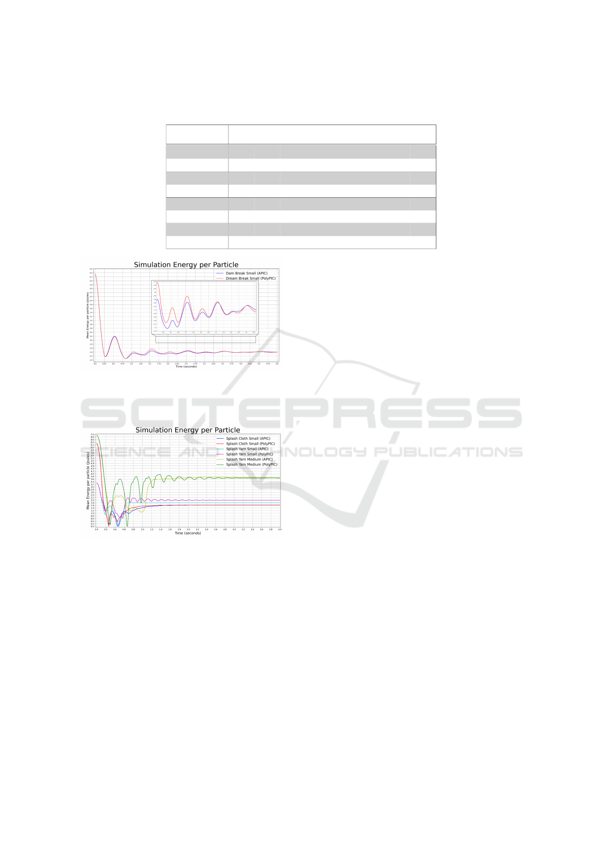
Table 2: Timing and storage data for APIC and PolyPIC for three example scenarios.

†

The dam break simulations involved

no fabric, so required 0 mesh/rod elements.

Example simulation

duration

(s)

timestep

(s)

s/step

(avg)

total

run time

(mins)

peak

memory

(GB)

#particles

(avg)

#ﬂuid

particles

(avg)

#elements

(avg)

Dam Break Small

(APIC)

5.0 0.0002 0.510 217 1.978 310929 310929 0

†

Dam Break Small

(PolyPIC)

5.0 0.0002 1.172 499 2.040 310839 310839 0

†

Splash Cloth Small

(APIC)

4.0 0.0002 0.480 167 0.896 12359 1360 20406

Splash Cloth Small

(PolyPIC)

4.0 0.0001 0.428 282 0.842 12228 1228 20406

Splash Yarn Small

(APIC)

4.0 0.0002 0.454 155 1.056 23074 3471 19799

Splash Yarn Small

(PolyPIC)

4.0 0.0002 0.579 197 1.109 23233 3630 19799

Splash Yarn Medium

(APIC)

4.0 0.0002 1.897 818 9.300 119520 40320 79596

Splash Yarn Medium

(PolyPIC)

4.0 0.00005 1.460 1958 5.764 116416 37213 79596

Figure 8: Mean particle energy for the dam break scenario,

calculated as the sum of kinetic energy and gravitational

potential energy. PolyPIC improves the energy preservation

over APIC, but the effect per particle is minor.

Figure 9: Mean particle energy for the interaction scenarios,

calculated as the sum of kinetic energy and gravitational po-

tential energy. Change in energy preservation in PolyPIC

and APIC is minimal, although the energy of PolyPIC os-

cillates for a longer period before reaching a constant value.

Due to differences in the simulation setup (e.g. fabric at

different world heights, rigid sphere in cloth scenario), each

simulation stabilises around a different ﬁnal mean energy.

namics. Whilst theoretically PolyPIC has been shown

to be lossless when transferring velocity between the

particles and the grid (shown in the supplementary

material of Fu et al), this can’t be achieved in prac-

tice. For ﬂuids, using polynomial modes involving

multi-quadratic terms (i.e. N

> 2

) causes the sim-

ulation to become unstable, even when a very small

time step is used. For solids in a non-coupled sce-

nario, the maximum number of modes can be used

without effecting the overall stability of the simula-

tion. However, when simulating coupled interaction,

stability issues become increasingly severe as higher

order modes are introduced.

As can be seen in Table 2, when comparing the

dam break scenarios, an increase in the time required

for each simulation step can be seen when using

PolyPIC rather than APIC. In the interaction scenar-

ios, the time per simulation generally decreases, but

the average number of ﬂuid particles in the simulation

also decreases. The reduced numerical damping of

PolyPIC causes the ﬂuid to splash off the fabric rather

than being absorbed, so the ﬂuid particles leave the

domain of the simulation faster, and the particles are

deleted from the simulation. This reduces the number

of ﬂuid particles to be simulated in later timesteps,

allowing each step to be simulated faster.

The fabric-interaction simulations for APIC were

both able to be simulated using a timestep of ∆t =

−4

s, but using this value for the PolyPIC scenarios

caused the simulation to become unstable. Whilst the

same timestep enabled stable simulation of the small

yarn PolyPIC scenario, we found using a timestep of

∆t = 1e

−4

s and ∆t = 5e

−5

s allowed the small cloth

and medium yarn PolyPIC simulation to remain sta-

ble for their duration, respectively. This means that

while in general there was only a small change in the

time required for each simulation step, the need for

a smaller timestep for PolyPIC resulted in an overall

increase in the time taken to run the simulation, as

shown in Table 2.

Possible future work would be to experiment with

more stable simulation frameworks such as position-

based dynamics (M

uller et al., 2007) which has been

shown to reduce the need for small timesteps. Also,

in the yarn examples, the individual yarns quickly be-

come tangled after collision with the ﬂuid. Using a

more robust collision handling technique such as in-

cremental potential contact (Li et al., 2020) could im-

prove the stability of the simulations.

GRAPP 2024 - 19th International Conference on Computer Graphics Theory and Applications

250

6 CONCLUSIONS

The work presented by Fei et al is widely consid-

ered to be the state-of-the-art for liquid-fabric inter-

action simulations. This paper has replaced APIC

with PolyPIC in their model and performed a com-

parison of the PolyPIC model with the APIC model

in the context of liquid-fabric interactions. Using

PolyPIC in place of APIC for liquid-fabric interac-

tion improves the dynamism of simulations, increas-

ing energy transfer between the ﬂuid and cloth/yarn

and increasing the resolution of vorticial details and

small scale splashes. However, PolyPIC has a higher

computation cost over APIC and the reduced numer-

ical damping of PolyPIC also caused stability issues

requiring the use of a smaller time step. This require-

ment for smaller timesteps highlights the need for a

greater consideration of techniques to improve simu-

lation stability and inter-yarn collision detection. De-

spite this limitation, this paper demonstrates the po-

tential of PolyPIC as a method of improving liquid-

fabric interaction simulations based on PIC methods.

ACKNOWLEDGEMENTS

This research is supported by a Frank Greaves Simp-

son Scholarship from the University of Shefﬁeld.

REFERENCES

Bergou, M., Wardetzky, M., Robinson, S., Audoly, B., and

Grinspun, E. (2008). Discrete elastic rods. ACM

Transactions on Graphics, 27(3):1–12.

Brackbill, J. and Ruppel, H. (1986). FLIP: A method for

adaptively zoned, particle-in-cell calculations of ﬂuid

ﬂows in two dimensions. Journal of Computational

Physics, 65:314–343.

Fang, Y., Li, M., Gao, M., and Jiang, C. (2019). Silly rub-

ber: an implicit material point method for simulating

non-equilibrated viscoelastic and elastoplastic solids.

ACM Transactions on Graphics, 38:1–13.

Fei, Y. R., Batty, C., Grinspun, E., and Zheng, C. (2018). A

multi-scale model for simulating liquid-fabric interac-

tions. ACM Trans. Graph., 37(4).

Fu, C., Guo, Q., Gast, T., Jiang, C., and Teran, J. (2017).

A polynomial particle-in-cell method. ACM Transac-

tions on Graphics, 36(6):222:1–222:12.

Grinspun, E., Hirani, A., Desbrun, M., and Schr

oder, P.

(2003). Discrete Shells. In Proceedings of the 2003

ACM SIGGRAPH/Eurographics Symposium on Com-

puter Animation.

Harada, T., Koshizuka, S., and Kawaguchi, Y. (2007). Real-

time Fluid Simulation Coupled with Cloth. EG UK

Theory and Practice of Computer Graphics.

Harlow, F. H. (1962). The particle-in-cell method for nu-

merical solution of problems in ﬂuid dynamics. Tech-

nical Report LADC-5288.

Huber, M., Pabst, S., and Straßer, W. (2011). Wet cloth

simulation. In International Conference on Computer

Graphics and Interactive Techniques.

Jiang, C., Schroeder, C., Selle, A., Teran, J., and Stomakhin,

A. (2015). The afﬁne particle-in-cell method. ACM

Transactions on Graphics, 34(4):51:1–51:10.

Lenaerts, T., Adams, B., and Dutr

e, P. (2008). Porous

ﬂow in particle-based ﬂuid simulation. ACM Trans.

Graph., 27.

Li, M., Ferguson, Z., Schneider, T., Langlois, T., Zorin,

D., Panozzo, D., Jiang, C., and Kaufman, D. M.

(2020). Incremental potential contact: intersection-

and inversion-free, large-deformation dynamics. ACM

Transactions on Graphics, 39(4).

uller, M., Heidelberger, B., Hennix, M., and Ratcliff,

J. (2007). Position based dynamics. Journal of

Visual Communication and Image Representation,

18(2):109–118.

Nielsen, M. B. and Østerby, O. (2013). A two-continua

approach to Eulerian simulation of water spray. ACM

Transactions on Graphics, 32(4):1–10.

Patkar, S. and Chaudhuri, P. (2013). Wetting of Porous

Solids. IEEE Transactions on Visualization and Com-

puter Graphics, 19(9):1592–1604.

Shao, X., Wu, W., and Wang, B. (2018). Position-based

simulation of cloth wetting phenomena. Computer

Animation and Virtual Worlds, 29(1):e1788.

SideFX (2023). Houdini - 3D modeling, animation, VFX,

look development, lighting and rendering | SideFX.

Stomakhin, A., Schroeder, C., Chai, L., Teran, J., and Selle,

A. (2013). A material point method for snow simula-

tion. ACM Transactions on Graphics, 32(4):1–10.

Stomakhin, A., Schroeder, C., Jiang, C., Chai, L., Teran,

J., and Selle, A. (2014). Augmented MPM for phase-

change and varied materials. ACM Transactions on

Graphics, 33(4):1–11.

Sulsky, D., Chen, Z., and Schreyer, H. L. (1994). A par-

ticle method for history-dependent materials. Com-

puter Methods in Applied Mechanics and Engineer-

ing, 118(1):179–196.

Zheng, Y., Chi, X., Chen, Y., and Wu, E. (2021). Stains on

imperfect textile. Virtual Reality & Intelligent Hard-

ware, 3:142–155.

Using the Polynomial Particle-in-Cell Method for Liquid-Fabric Interaction

251