
Determination of Factors of Interest in Bone Models Based on
Ultrasonic Data
Marija Chuchalina, Aleksandrs Sisojevs
a
and Alexey Tatarinov
b
Institute of Electronics and Computer Science, 14 Dzerbenes Str., Riga, Latvia
Keywords: Machine Learning, Factor of Interest, Bone Model, Ultrasound, Signal Processing.
Abstract: Osteoporosis is characterized by increased bone fragility due to a decrease in thickness of the cortical layer
CTh and the development of internal porosity in it. The assessment of bone models that simulate the state of
osteoporosis causes difficulties due to their complex and multi-layered structure. In the present work, the
possibility of using machine learning approaches to determine internal porosity using the ultrasonic data
obtained by scanning bone models was researched. The bone models were represented as sets of PMMA
plates with gradually varying CTh from 2 to 6 mm. A stepwise progression of porosity from 0 to 100% of
CTh was set by increasing the thickness of the porous layer PTh in steps of 1 mm. The evaluation method
was based on the results of the supervised multi-class classification of the raw ultrasonic signals and their
magnitude of the DFT spectrum with PTh used for labeling. Ultrasonic data was split into training and testing
datasets while preserving the percentage of samples for each class. The results of the experiments
demonstrated the potential effectiveness of the PTh classification, while optimization of the datasets and
additional signal processing may contribute to the improvement of the results.
1 INTRODUCTION
Osteoporosis is a systemic skeletal disease
characterized by low bone density and
microarchitectural deterioration of bone tissue with a
consequent increase in bone fragility. The
cornerstone of diagnosis is the measurement of bone
mineral density (WHO, 2003). The condition of
cortical bone and the development of osteoporosis are
determined by many mechanical, microstructural,
and macrostructural bone properties, such as
hardness, porosity, and cortical thickness.
For several years, there has been progress in the
development of axial transmission quantitative
ultrasound (QUS) technologies for the evaluation of
long bones using a variety of acoustic wave modes
(Laugier, 2008). QUS has the potential to predict
fracture risk in several clinical settings and has
multiple advantages. It is non-ionizing, cost-
effective, portable, and has the potential to become an
effective complement or alternative to
osteodensitometry (DXA), which is currently the
“gold standard” for diagnosing osteoporosis.
a
https://orcid.org//0000-0002-2267-4220
b
https://orcid.org//0000-0002-5787-2040
However, neither existing bone QUS nor DXA are
able to reliably distinguish between changes
associated with the thinning of the bone cortex and
the increase of intracortical porosity, which are the
main factors of bone fragility. Thus, differentiation
between a thin healthy bone and an osteoporotic one
is problematic. Recent approaches focus on the
analysis of guided wave propagation at multiple
frequencies, which provides extensive information on
bone structure and properties (Tatarinov et al., 2014).
Nevertheless, discrimination of factors of interest
such as intracortical porosity and thickness of cortical
layer against the background of effects surrounding
soft tissue requires advanced data processing
(Sisojevs et al., 2023).
In the field of deep machine learning, there is a
growing interest in recurrent neural networks
(RNNs), which have been used for many sequence
modeling tasks. They have achieved promising
performance improvements in multiple technical
applications such as speech recognition, human
activity recognition, medical signal evaluation, and
many other sequence classification tasks (Graves,
Chuchalina, M., Sisojevs, A. and Tatarinov, A.
Determination of Factors of Interest in Bone Models Based on Ultrasonic Data.
DOI: 10.5220/0012358500003654
Paper published under CC license (CC BY-NC-ND 4.0)
In Proceedings of the 13th International Conference on Pattern Recognition Applications and Methods (ICPRAM 2024), pages 281-287
ISBN: 978-989-758-684-2; ISSN: 2184-4313
Proceedings Copyright © 2024 by SCITEPRESS – Science and Technology Publications, Lda.
281

2012; Li et al., 2020; Murad & Pyun, 2017). The
reason for their effectiveness in the solution of
sequence-based tasks is their ability to use contextual
information and learn the temporal dependencies of
the input data (Murad & Pyun, 2017). However, a
lack of research related to the determination of
cortical bone thickness and/or porous layer thickness
in ultrasound data using machine learning approaches
was observed.
The purpose of this study was to explore the
possibility of determining one of the factors of
interest - intracortical porosity against the
background of changes in cortical thickness using
ultrasonic data in bone models. Ultrasonic signals
were obtained by axial scanning synthetic phantoms
of cortical bone simulating changes in cortical
thickness and progression of intracortical porosity.
The raw data was presented by sets of ultrasonic
signals acquired stepwise by surface profiling of the
bone phantoms in the pitch-catch mode (Sisojevs et
al., 2023). Both raw ultrasonic signals in the time
domain and signals processed by discrete Fourier
transformation (DFT) were used as input data in
separate experiments for machine learning tasks. DFT
is one of the recognized methods of signal analysis
that transforms signals from time to frequency
domains (Stone, 2021). A multi-metric approach was
implemented to evaluate the results obtained in both
experiments. This included not only the precise
classification of samples, but also the evaluation of
their neighbor’s predictions. This is due to the
complexity and volume of the input data, as well as
the need to gain a better understanding of
classification accuracy.
2 PROPOSED APPROACH
Intracortical porosity was specified by the thickness
of the porous layer PTh, which increased discretely
from the inner (lower) surface of the bone phantom to
the outer (upper) surface. The proposed approach for
evaluating PTh was based on supervised machine
learning methods. To perform multi-class
classification, two types of ultrasonic data in bone
models were prepared for machine learning tasks,
data and label arrays were created and split into
training and testing sets, and training and testing were
performed to assess the performance of the approach.
2.1 Input Data Acquisition and
Pre-Processing
The bone models or phantoms were represented as
sets of bi-layer acrylic plates with gradually varying
total thicknesses simulating the bone cortical
thickness CTh from 2 to 6 mm with a step of 1 mm.
The effect of intracortical porosity, progressing from
the bone canal, was mimicked by regularly bottom-
drilled holes. A step change in porosity in the
phantom volume from 0 to 100% CTh was set by
increasing the thickness of the porous layer PTh in
increments of 1 mm. The phantoms were covered
with soft tissue with thicknesses of 0, 2 and 4 mm.
Ultrasonic signals were acquired using a custom-
made scanning device by stepwise profiling the upper
surface of the phantoms covered with soft tissue. The
profiling step was 3 mm. In total, the 24 obtained
signals formed the so-called ultrasonic
spatiotemporal wave profiles. The profiles contained
complex information about the temporal (velocity)
and energetic (attenuation) characteristics of different
types of ultrasound propagation. (Sisojevs et al.,
2023). A total of 1800 samples of the ultrasonic signal
were acquired. One signal frame with a duration of 1
ms contains the responses of three ultrasonic
excitation regimes: high frequency (500 kHz), low
frequency (100 kHz) and chirp mode (from 50 to 500
kHz). In this frequency range, different modes of
ultrasonic guided waves are manifested. For
comparison purposes, 2 sets of data – raw signals and
DFT-processed signals, were created. In regard to
DFT processing, each of the discrete signals was
transformed into a spectral signal that described the
magnitude spectrum.
(1)
where:
– signal at = 0…
;
– Nth root of unity.
(2)
where:
– real component of the spectral signal;
– imaginary component of the spectral
signal.
Informative regions were extracted for use in
machine learning tasks, thus creating a set of features
that characterize the signals. In our case, a single
feature corresponded to one discrete sample of the
ultrasonic signal in the selected informative region.
These regions consisted of 3000-5000 features for the
raw dataset and 750 features for the DFT-transformed
dataset. The values in signal datasets were
ICPRAM 2024 - 13th International Conference on Pattern Recognition Applications and Methods
282
normalized. The vector of class labels for multi-class
classification represented by an integer was converted
to one-hot encoding, which represented the
categorical variables as a binary vector. The values in
the binary vector are denoted by 0 except for the
integer index, which is denoted by 1. It should have
also been taken into account that the number of
samples for each of the classes is not equal due to the
nature of the acquired ultrasonic data. The largest
number of samples is at PTh <= 2, while the smallest
is at PTh = 6.
2.2 Machine Learning Methods
The proposed machine learning methods included the
bidirectional Long Short-Term Memory (BLSTM)
deep neural network model, which is a type of RNN
specifically designed to process sequential data and is
able to capture long-term dependencies in it, as well
as classical machine learning algorithms for
supervised multi-class classification.
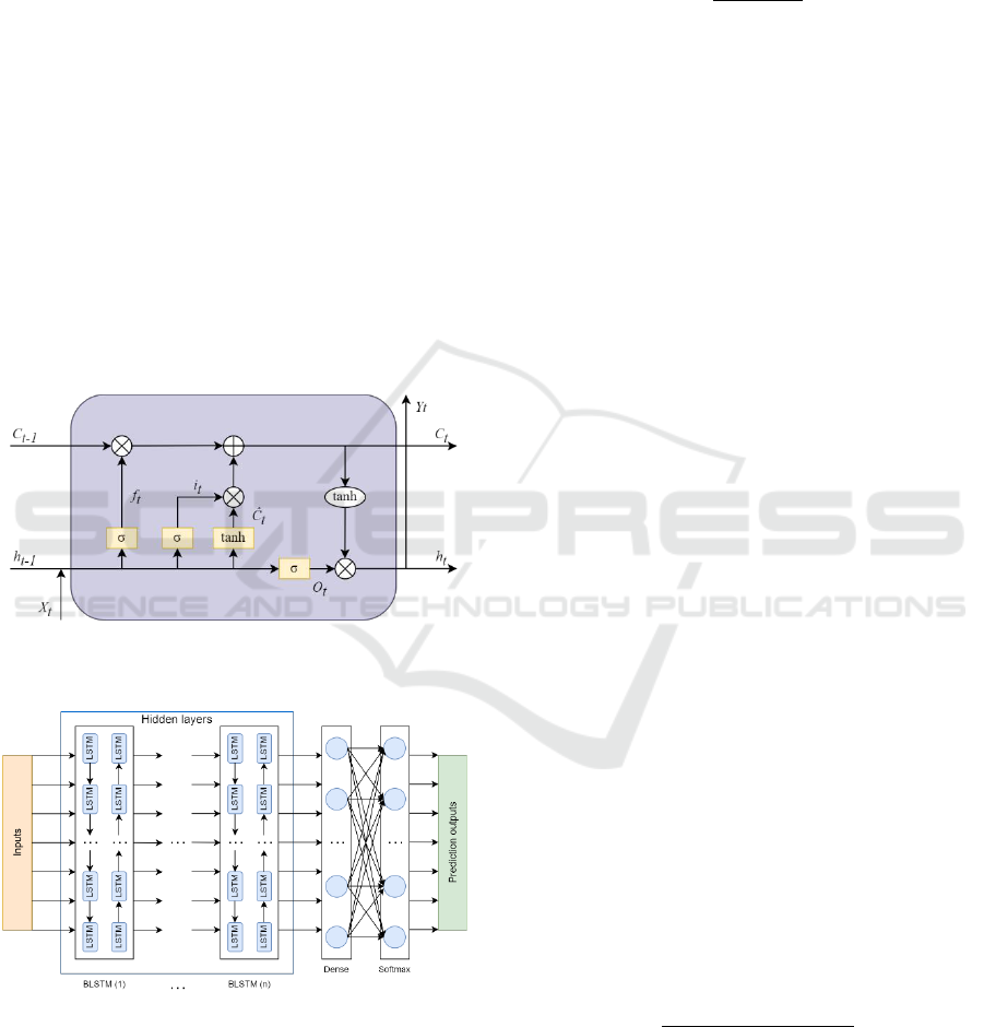
Figure 1: Schematic diagram of the LSTM memory unit
(Aggarwal, 2023; Sun, J. et al., 2019).
Figure 2: Structure of the deep BLSTM network (Zhang et
al., 2021).
The architecture of the applied artificial neural
network is illustrated in Figure 1 and Figure 2, where:
– input time step;
– output;
– cell state;
–
forget gate;
– input gate;
– output gate;
–
internal cell state.
The model utilized a softmax activation function
that converts a vector of values into a probability
distribution that can be interpreted as class
membership probabilities. The elements of the output
vector are in the range (0, 1) and sum to 1.
(3)
where:
– input vector;
– Euler's number;
– index of the value for which the exponent is
calculated;
– number of probabilities in the probability
distribution.
In conjunction with the softmax activation
function, cross-entropy, which computes a score that
summarizes the average difference between the actual
and predicted probability distributions for all classes,
was used as the loss function for multi-class
classification tasks. The function requires the output
layer to be configured with n nodes, where n is the
number of classes. The experiments within the given
work involved 7 classes corresponding to 7 possible
thicknesses of the porous layer PTh varying from 0
mm to 6 mm.
The classical machine learning algorithms
provided by the machine learning framework enabled
simultaneous testing of different machine learning
models and were used as part of the study to evaluate
and compare the results, verifying the performance of
the proposed approach.
2.3 Evaluation Methods
To evaluate the results obtained during the
experiments, a multi-metric approach was
introduced, which included the interpretation of the
precise classification of samples, as well as the
assessment of their neighbors’ predictions. The latter
enabled a more granular method for the examination
of the results taking into consideration the complexity
and volume of the input data.
Accuracy metric was used to define the ratio of
correctly classified samples to the total number of
samples.
(4)
where:
( ) – number of correct matches;
( ) – number of correct
mismatches;
( ) – number of incorrect
matches;
Determination of Factors of Interest in Bone Models Based on Ultrasonic Data
283

( ) – number of incorrect
mismatches.
Recall metric TPR was used to define the ratio of
correctly classified positive samples to the total
number of positive samples.
(5)
where:
( ) – number of correct matches;
( ) – number of incorrect
mismatches.
Precision metric PPV was used to define the ratio
of correctly classified positive samples to the total
predicted number of positive samples.
(6)
where:
( ) – number of correct matches;
( ) – number of incorrect
matches.
Loss metric was used to summarize the mean
difference between the actual and predicted
probability distributions for all classes in the machine
learning tasks, while F1-score displayed model
performance.
(7)
where:
( ) – number of correct matches;
( ) – number of incorrect
matches;
( ) – number of incorrect
mismatches.
Accuracy and related metrics alone are not
sufficient to fully evaluate model performance results
in a given classification context. Due to the
significant complexity of the data structure of
ultrasonic signals, slight deviations from the ideal
prediction were acceptable. To obtain a more
complete perspective, additional custom metrics were
implemented in scope of the present work to evaluate
the neighbors of the classified classes. The result can
be considered satisfactory if most of the classes were
predicted correctly and most of the neighbors that are
deviations from the ideal result are within a range that
does not exceed the specified limit ∆ <= 2 mm.
Based on the actual and predicted classes, a custom
so-called accuracy_2 metric was developed. Its
purpose was to show how often each of the classes
had deviations for each deviation value in
millimeters. Parameter's ∆ of accuracy_2 metric
value was calculated as the modulus of the difference
between the actual and predicted values and ranged
from 0 to 6 millimeters, respectively.
(8)
where:
– actual class value in millimeters;
– predicted class value in millimeters.
After calculating the values of ∆ and writing
them into the array D, the number of differences in
the specified range for each of the classes was
determined and written into the matrix A.
(9)
where:
– element that satisfies the condition;
– row index of matrix A;
– column index of matrix A;
– array of actual class values;
– array of values.
An additional metric accuracy_2(%) based on
accuracy_2 that takes into account the ratio of the
number of samples of each class was introduced. For
each - class in its row, - the ratio of its ∆ value
to the total number of ∆ values for that class is
calculated, which is then multiplied by 100 to obtain
a percentage value.
(10)
where:
– matrix A element;
– row index of matrix A;
– column index of matrix A;
– the number of values in the -th row of matrix A.
The results were then rounded using the largest
remainder method.
During the process of interpretation of the
accuracy_2(%) metric, attention was paid to the
elements located on the left side of the resulting heat
map. A bigger number of elements on the left side of
the heatmap signified better performance of the
trained model. A range of colors from green to red
was used for visualization, with green indicating the
biggest number of elements and red indicating the
smallest number of elements.
3 EXPERIMENTS
As part of the validation of the proposed approach,
experiments were carried out to determine PTh using
labeled raw and DFT-transformed sets of data
separately. In the experiments, various BLSTM
model configurations (1, 2 and 3 hidden layers) and
ICPRAM 2024 - 13th International Conference on Pattern Recognition Applications and Methods
284
hyperparameter sets were assessed to observe their
impact on the performance of the model. A
hyperparameter optimization framework was utilized
to determine the optimal set of hyperparameters. The
top performance results were achieved with the batch
size = 32 and learning rate = 0.001, as well as 80%
training and 20% test dataset ratio.
Both the deep neural network and several classical
machine learning models implemented in the
machine learning framework, such as
ExtraTreesClassifier, AdaBoostClassifier,
RandomForestClassifier, etc., failed to effectively
classify the thickness of the porous layer PTh of the
bone models.
Classical machine learning models demonstrated
21.67 – 29.17% accuracy, 0.2057 – 0.2929 F1-score
for each soft tissue layer separately and 25.28%
accuracy, 0.2316 F1-score for all the soft tissue layers
together.
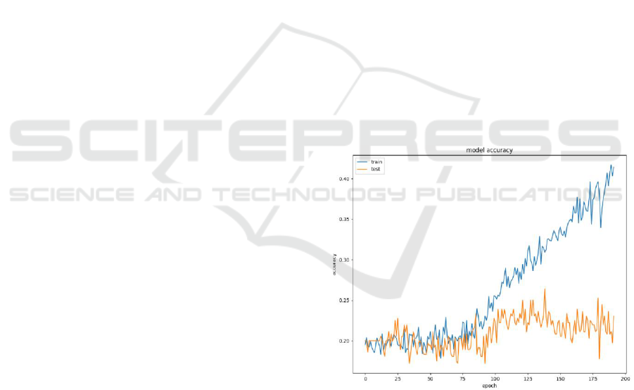
The BLSTM model struggled to determine
dependencies among large arrays of raw ultrasonic
data features (Figure 4 - 6), reaching ~26% accuracy
(Figure 3), 0.23 precision, 0.26 recall and 0.23 F1-
score. Thus, the experimental results for raw
ultrasonic signal data were considered unsatisfactory.
Experiments with DFT-transformed ultrasonic
signals showed better results than experiments with
raw signals.
Classical machine learning models, such as SVC,
KNeighborsClassifier, ExtraTreesClassifier,
LGBMClassifier, etc., demonstrated 70.83 – 75.83%
accuracy, 0.6949 – 0.7611 F1-score for each soft
tissue layer separately and 68,61% accuracy, 0.6823
F1-score for all the soft tissue layers together.
The BLSTM model achieved better results with 3
hidden layers (Figure 8 - 9) and showed ~56%
accuracy (Figure 7), 0.57 precision, 0.56 recall and
0.55 F1-score. Examination of the rest of the
predictions using the custom accuracy_2 and
accuracy_2(%) metrics (Figure 10) revealed that most
of them are nearest neighbors of the exact predictions
in the range of ∆<=2 mm and are concentrated on
the left side of the heatmap with a few exceptions as
demonstrated in Figure 10. Classes with the largest
number of samples in the dataset were predicted best
at PTh<=3, with the predictions getting progressively
worse as the number of samples in the dataset
decreased.
Both machine learning approaches showed that a
smaller amount of features in the case of DFT-
transformed ultrasonic signal data (750 inputs)
contributed to a more accurate classification of the
thickness of the porous layer PTh.
Upon evaluation of the BLSTM model’s
performance, an overfitting problem was observed,
despite the introduction of Dropout and
EarlyStopping to prevent it. This indicates the need
for further optimization of the dataset and model.
Classical machine learning methods achieved better
results with each value of the soft tissue layer
thickness separately, whereas the deep neural
network worked better with all soft tissue layer
thickness values together.
The following computer system was used to
implement the experiments: Intel Core i7-12700H,
Nvidia RTX 3070 Ti, 8GB with 5888 CUDA cores,
RAM 32.0 GB, JetBrains PyCharm 2022.3.2 IDE,
Anaconda virtual environment with Python 3.10,
CUDA Toolkit 11.2.2 and CuDNN 8.1.0.
Experiments were run utilizing the GPU
computing power for model training and testing. With
all the prerequisites complete, TensorFlow in
conjunction with Keras enabled transparent GPU
usage without explicit code configuration, thus
facilitating operations to be run on GPU by default.
Considering the above, CuDNN is automatically used
with the LSTM layer, starting with Tensorflow 2.x.
Nvidia CUDA parallel computing platform and
CuDNN library for deep neural networks gave an
increase of more than 90% in system performance.
Figure 3: Model accuracy with raw ultrasonic data.
Determination of Factors of Interest in Bone Models Based on Ultrasonic Data
285
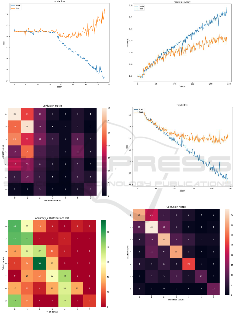
Figure 4: Model loss with raw ultrasonic data.
Figure 5: Confusion matrix with raw ultrasonic data.
Figure 6: Accuracy_2(%) distributions with raw ultrasonic
data.
Figure 7: Model accuracy with DFT ultrasonic data.
Figure 8: Model loss with DFT ultrasonic data.
Figure 9: Confusion matrix with DFT ultrasonic data.
ICPRAM 2024 - 13th International Conference on Pattern Recognition Applications and Methods
286
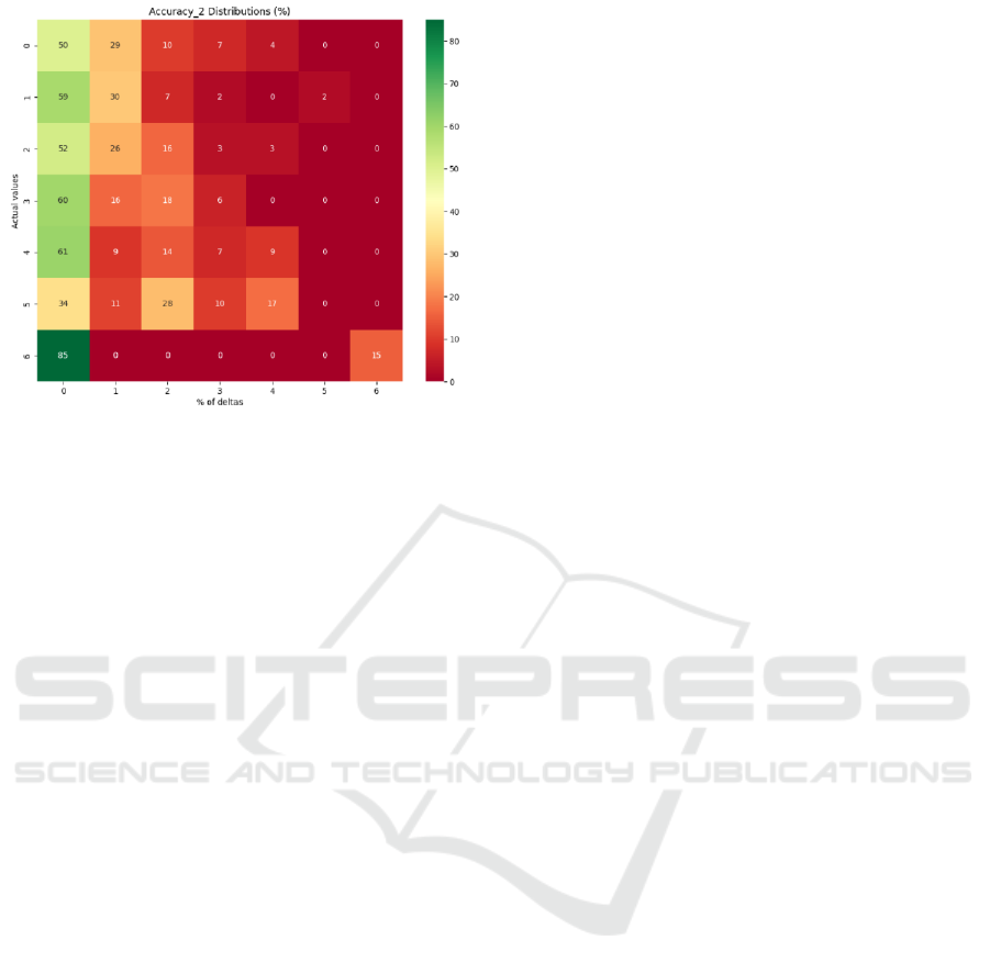
Figure 10: Accuracy_2(%) distributions with DFT
ultrasonic data.
4 CONCLUSIONS
The results of the experiments demonstrated the
potential effectiveness of the proposed method in
machine learning tasks for determining the thickness
of the inner porous layer PTh of the bone cortex as
the factor of interest in osteoporosis diagnostics using
ultrasonic data. The results were obtained in the
presence and disrespectfully of surrounding soft
tissues up to 4 mm thick that is one of the main
artefacts in bone QUS. The use of the DFT-processed
ultrasonic signals as inputs for machine learning
provides higher accuracy of classification as opposed
to the raw ultrasonic signals. The present dataset does
not allow to have higher model performance,
however, experiment outcomes indicate a potential
for accuracy improvements with expansion and
optimization of the datasets, as well as additional
signal processing, which may contribute to the
representativeness of the datasets.
ACKNOWLEDGMENTS
The study was executed under the project of the
Latvian Council of Science LZP FLPP no. lzp -
2021/1-0290 "Comprehensive assessment of the
condition of bone and muscle tissue using
quantitative ultrasound (BoMUS)”.
REFERENCES
WHO Scientific Group (2003). Prevention and
management of osteoporosis: report of a WHO
scientific group. WHO Technical Report Series 921.
Laugier P. (2008). Instrumentation for in vivo ultrasonic
characterization of bone strength. IEEE transactions on
ultrasonics, ferroelectrics, and frequency control.
55(6):1179-96.
Tatarinov, A., Egorov V., Sarvazyan A., Sarvazyan N.
(2014) Multi-frequency axial transmission bone
ultrasonometer. Ultrasonics. 54(5), 1162-1169.
Sisojevs, A., Tatarinov, A., Chaplinska, A. (2023).
Evaluation of factors-of-interest in bone mimicking
models based on DFT analysis of ultrasonic signals.
ICPRAM 2023: 914-919.
Graves, A. (2012). Supervised Sequence Labelling with
Recurrent Neural Networks. Springer. ISBN: 978-3-
642-24797-2.
Li, Y. H., Harfiya, L. N., Purwandari, K., Lin, Y. (2020).
Real-Time Cuffless Continuous Blood Pressure
Estimation Using Deep Learning Model. Machine
Learning for Sensing and Healthcare 2020-2021.
20(19), 5606.
Murad, A., Pyun, J.Y. (2017). Deep Recurrent Neural
Networks for Human Activity Recognition. Sensor
Signal and Information Processing. 17(11), 2556.
Stone, J. V. (2021). The Fourier Transform: A Tutorial
Introduction. Sebtel Press. 103 p.
Aggarwal, S. (2023). The Ultimate Guide to Building Your
Own LSTM Models. ProjectPro.
Sun, J., Shi, W., Yang, Z., Yang, J., Gui, G. (2019).
Behavioral Modeling and Linearization of Wideband
RF Power Amplifiers Using BiLSTM Networks for 5G
Wireless Systems. IEEE Transactions on Vehicular
Technology. 68(11), 10348-10356.
Zhang, Y., Zhao, Z., Deng, Y., Zhang, X., Zhang, Y.
(2021). Heart biometrics based on ECG signal by sparse
coding and bidirectional long short-term memory.
Multimedia Tools and Applications. 80(1), 30417–
30438.
Determination of Factors of Interest in Bone Models Based on Ultrasonic Data
287
