Association of Grad-CAM, LIME and Multidimensional Fractal

Techniques for the Classiﬁcation of H&E Images

Thales R. S. Lopes

, Guilherme F. Roberto

2 a

, Carlos Soares

2 b

, Tha

ına A. A. Tosta

3 c

Adriano B. Silva

4 d

, Adriano M. Loyola

, S

ergio V. Cardoso

5 e

, Paulo R. de Faria

6 f

Marcelo Z. do Nascimento

4 g

and Leandro A. Neves

1 h

Department of Computer Science and Statistics, S

ao Paulo State University, S

ao Jos

e do Rio Preto-SP, Brazil

Faculty of Engineering, University of Porto, Porto, Portugal

Institute of Science and Technology, Federal University of S

ao Paulo, S

ao Jos

e dos Campos-SP, Brazil

Faculty of Computer Science, Federal University of Uberl

andia, Uberl

andia-MG, Brazil

Area of Oral Pathology, School of Dentistry, Federal University of Uberl

andia, Uberl

andia-MG, Brazil

Department of Histology and Morphology, Institute of Biomedical Science,

Federal University of Uberl

andia, Uberl

andia-MG, Brazil

Keywords:

Deep Learning, Fractal Features, Explainable Artiﬁcial Intelligence, Histological Images.

Abstract:

In this work, a method based on the use of explainable artiﬁcial intelligence techniques with multiscale

and multidimensional fractal techniques is presented in order to investigate histological images stained with

Hematoxylin-Eosin. The CNN GoogLeNet neural activation patterns were explored, obtained from the

gradient-weighted class activation mapping and locally-interpretable model-agnostic explanation techniques.

The feature vectors were generated with multiscale and multidimensional fractal techniques, speciﬁcally frac-

tal dimension, lacunarity and percolation. The features were evaluated by ranking each entry, using the ReliefF

algorithm. The discriminative power of each solution was deﬁned via classiﬁers with different heuristics. The

best results were obtained from LIME, with a signiﬁcant increase in accuracy and AUC rates when compared

to those provided by GoogLeNet. The details presented here can contribute to the development of models

aimed at the classiﬁcation of histological images.

1 INTRODUCTION

Clinical diagnoses and studies in the medical ﬁeld are

commonly based on biomedical images, a fact that

has motivated applications and research in the ﬁelds

of computer vision and pattern recognition (Zerdoumi

et al., 2018). Thus, it is possible to exploit a series

of characteristics present in this category of images,

such as microscopic information (texture, colour, and

morphology) of tissues and cells (Cruz-Roa et al.,

2011).

https://orcid.org/0000-0001-5883-2983

https://orcid.org/0000-0003-4549-8917

https://orcid.org/0000-0002-9291-8892

https://orcid.org/0000-0001-8999-1135

https://orcid.org/0000-0003-1809-0617

https://orcid.org/0000-0003-2650-3960

https://orcid.org/0000-0003-3537-0178

https://orcid.org/0000-0001-8580-7054

In this context, representation learning encom-

passes a set of techniques for automatically trans-

forming data, such as pixels in a digital image, into

a feature vector, with the aim of recognising existing

patterns in the domain under analysis. In this context,

models based on deep learning stand out among the

different representation learning approaches, as they

have multiple levels and can therefore learn highly

complex functions (LeCun et al., 2015). The increase

in computer processing capacity has made it possible

to exploit a speciﬁc type of deep learning approach,

known as a Convolutional Neural Network (CNN),

which has provided important advances in image pro-

cessing and pattern recognition (LeCun et al., 2015).

Computational models based on the deep learning

paradigm are proving effective in many applications,

such as the categorisation of medical images. The in-

terpretability of the results provided by deep neural

networks is still a challenge due to the ”black box”

Lopes, T., Roberto, G., Soares, C., Tosta, T., Silva, A., Loyola, A., Cardoso, S., R. de Faria, P., Z. do Nascimento, M. and Neves, L.

Association of Grad-CAM, LIME and Multidimensional Fractal Techniques for the Classiﬁcation of H&E Images.

DOI: 10.5220/0012358200003660

Paper published under CC license (CC BY-NC-ND 4.0)

In Proceedings of the 19th Inter national Joint Conference on Computer Vision, Imaging and Computer Graphics Theory and Applications (VISIGRAPP 2024) - Volume 2: VISAPP, pages

441-447

ISBN: 978-989-758-679-8; ISSN: 2184-4321

441

nature of CNNs (Adadi and Berrada, 2018; Doshi-

Velez and Kim, 2017). The black box problem refers

to the level of concealment of the internal compo-

nents of a system (Suman et al., 2010). In the context

of artiﬁcial intelligence and deep learning, the sys-

tem’s difﬁculty in generating an explanation of how

it reached a decision deﬁnes the black box problem.

In critical decisions, such as the indication of a di-

agnosis, it is important to know the reasons behind

them. Therefore, the concept of explainable artiﬁ-

cial intelligence (XAI) offers interesting solutions for

making the knowledge produced by a computational

model that exploits black box artiﬁcial intelligence

techniques more comprehensible.

To this end, speciﬁc techniques are being explored

to evaluate neural activation patterns in a CNN (Ma-

hendran and Vedaldi, 2016; Yosinski et al., 2015). For

instance, the values present in the ”average pooling”

layer of a CNN, applied as a structural regularising

strategy, can deﬁne the image regions commonly used

in the classiﬁcation process through the use of the

gradient-weighted class activation mapping (Grad-

CAM) techniques (Rajaraman et al., 2018; Reyes

et al., 2020) and locally-interpretable model-agnostic

explanation (LIME) (Rajaraman et al., 2018; Reyes

et al., 2020; Iam Palatnik de Sousa, 2019). On

the other hand, the literature also shows the suc-

cess of computer models developed using consol-

idated image processing techniques, such as those

used for handcrafted features extraction (Ivanovici

et al., 2009b; M. Sahini, 2014). These studies have

explored strategies based on ﬁrst and second order

analyses, such as fractal techniques called fractal di-

mension, lacunarity and percolation.

Finally, it is important to note that despite

the advances involving CNN models for investi-

gating diseases in histological images stained with

Haematoxylin-Eosin (H&E), there has not yet been

a proposal aimed at investigating the discriminative

power of regions provided by Grad-CAM and LIME

techniques via multidimensional fractal approaches.

Fractal techniques can be applied to quantify the neu-

ral activation representations of a CNN and provide

new classiﬁcations and interpretations of the results.

These associations are relevant contributions to the

classiﬁcation and pattern recognition of diseases com-

monly investigated from histological images, as well

as to the ﬁeld of machine learning. The knowledge

obtained can be used to support more comprehensible

computer systems.

In this project, H&E histological images were ex-

plored through quantiﬁcation with fractal strategies of

the representations provided by the Grad-CAM and

LIME techniques. Speciﬁcally, the aim was to: ob-

tain neural activation patterns using the Grad-CAM

and LIME techniques; quantify the representations

of neural activation with multiscale and multidimen-

sional fractal techniques; and deﬁne the discrimina-

tive power of the features obtained using recognised

classiﬁers in the ﬁeld of artiﬁcial intelligence.

2 MATERIALS AND METHODS

The method was structured into four main stages: ob-

taining the CNN’s activation patterns; generating fea-

ture vectors; ranking and selecting features; classify-

ing and identifying the best combinations. The ﬁrst

stage aimed to organise and deﬁne a set of images

representative of the original image dataset, but only

with the images obtained via LIME and Guided Grad-

CAM. The second stage was dedicated to quantising

the images with fractal techniques and composing the

feature vectors. The third stage explored the use of

the ReliefF algorithm to identify the most relevant de-

scriptors for the histological image classiﬁcation pro-

cess (Robnik-Sikonja and Kononenko, 2003). Finally,

in the fourth stage, each set of features was analysed

by collecting the performances achieved with the rele-

vant classiﬁcation algorithms. A summary of the pro-

posed method is shown in Figure 1 and the details of

each stage are in the following sections.

The method was applied to six public H&E his-

tological images datasets. The CR dataset consists

of histological images derived from 16 H&E stained

sections of stage T3 or T4 colorectal cancer (Sir-

inukunwattana et al., 2017). The histological sec-

tions were digitised into whole-slide images (WSI)

using a Zeiss MIRAX MIDI digitiser with a pixel

resolution of 0.465µm. The images were catego-

rized into benign or malignant groups. This study

used 151 images measuring 775 x 522 pixels, divided

into 67 benign cases and 84 malignant cases. The

OD dataset was built from 30 tongue tissue sections

from mice stained with H&E previously subjected to

a carcinogen during two experiments carried out in

2009 and 2010, duly approved by the Ethics Com-

mittee on the Use of Animals, under protocol num-

ber 038/39 at the Federal University of Uberl

andia.

A total of 66 histological images were obtained us-

ing a LeicaDM500 optical microscope at 400 magni-

ﬁcation, using the RGB colour model with a resolu-

tion of 2048 × 1536 pixels. This dataset consists of

74 healthy and 222 severe dysplasia samples (Silva

et al., 2022). The resolution of each image is 452

x 250 pixels. The LA dataset is composed of liver

tissue obtained from mice and consists of 521 im-

ages divided into four classes where each represents

VISAPP 2024 - 19th International Conference on Computer Vision Theory and Applications

442

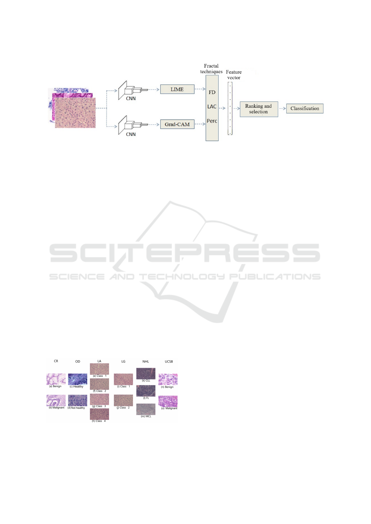
Figure 1: Illustration of the proposed method covering the phases: 1) Obtaining neural activation patterns; 2) Generating

feature vectors; 3) Ranking and selecting features; and 4) Classiﬁcation.

a group of female mice of different ages with ad li-

bitum diets: one (100), six (115), 16 (162) and 24

(152) months old. All the images have the same reso-

lution of 417 x 312 pixels. The LG dataset also con-

sists of images with dimensions of 417 x 312 pixels

representing liver tissue from mice. The two classes

represent the gender of the sample collected, totalling

265 examples: male with 150 images and female with

115 samples. Both LA and LG datasets were pro-

vided by the Atlas of Gene Expression in Mouse Ag-

ing Project (AGEMAP) (o. A. AGEMAP, 2020). The

NHL dataset consists of representative histological

images of three classes of non-Hodgkin’s lymphoma,

CLL, FL and MCL (do Nascimento et al., 2018). The

images were photographed and stored digitally with-

out compression in tif format, RGB colour model,

1388 x 1040 resolution and 24-bit quantization. A

total of 375 images were used, containing 113, 139

and 122 CLL, FL and MCL regions, respectively.

The UCSB dataset consists of 58 histological images

obtained from biopsies stained with Haematoxylin

and Eosin (H&E). All the images were made avail-

able by the University of California Santa Barbara

(Drelie Gelasca et al., 2008). The images have di-

mensions of 768 x 896 pixels, RGB colour standard

and 24-bit quantization rate. In Figure 2 samples of

the H&E datasets used in this work are shown.

Figure 2: Samples of the image datasets explored in this

paper.

The ﬁrst stage involves extracting neural activa-

tion patterns from a CNN. To this end, histological

images were analysed by applying the GoogLeNet

(Szegedy et al., 2015) model, pre-trained on the Im-

ageNet (He et al., 2016) dataset. This model was

chosen based on its performance in relation to that

achieved by different CNN architectures for classi-

fying histological H&E images. The model cho-

sen was the one with the lowest distinction rate, in

order to verify whether the proposed methodology

provides relevant gains in the image distinctions ex-

plored. Other models have been tested and could be

applied to deﬁne higher classiﬁcation rates. However,

the choice of the architecture with the lowest perfor-

mance effectively illustrates the worst-case gains via

the proposed model. This fact can guarantee new

strategies through less deep and complex models. The

tested models and the metrics applied are shown in

Table 1.

For each dataset, the ﬁne-tuning method was used

to adjust the output layer of the GooLeNet model to

the number of classes, with a learning rate of 0.001, a

momentum of 0.9 and the dataset was split in 80% to

train and 20% to validate the model.

After running the GoogLeNet model, the neural

activation patterns of the histological images were ob-

tained using the Guided Grad-CAM and LIME tech-

niques. Examples of representations obtained using

these techniques are shown in Figure 3.

The feature vectors were generated by applying

multiscale and multidimensional fractal techniques,

which can quantify self-similarity properties in im-

ages: these properties can be observed in histologi-

cal images and in the growth pattern of some tumours

(Baish and Jain, 2000). Fractal techniques have been

applied to quantify different types of lesions in histo-

logical images, especially multiscale and multidimen-

sional approaches such as fractal dimension, lacunar-

ity and percolation (Ivanovici et al., 2009a; Sahini and

Sahimi, 2014). The multiscale and multidimensional

Association of Grad-CAM, LIME and Multidimensional Fractal Techniques for the Classiﬁcation of H&E Images

443

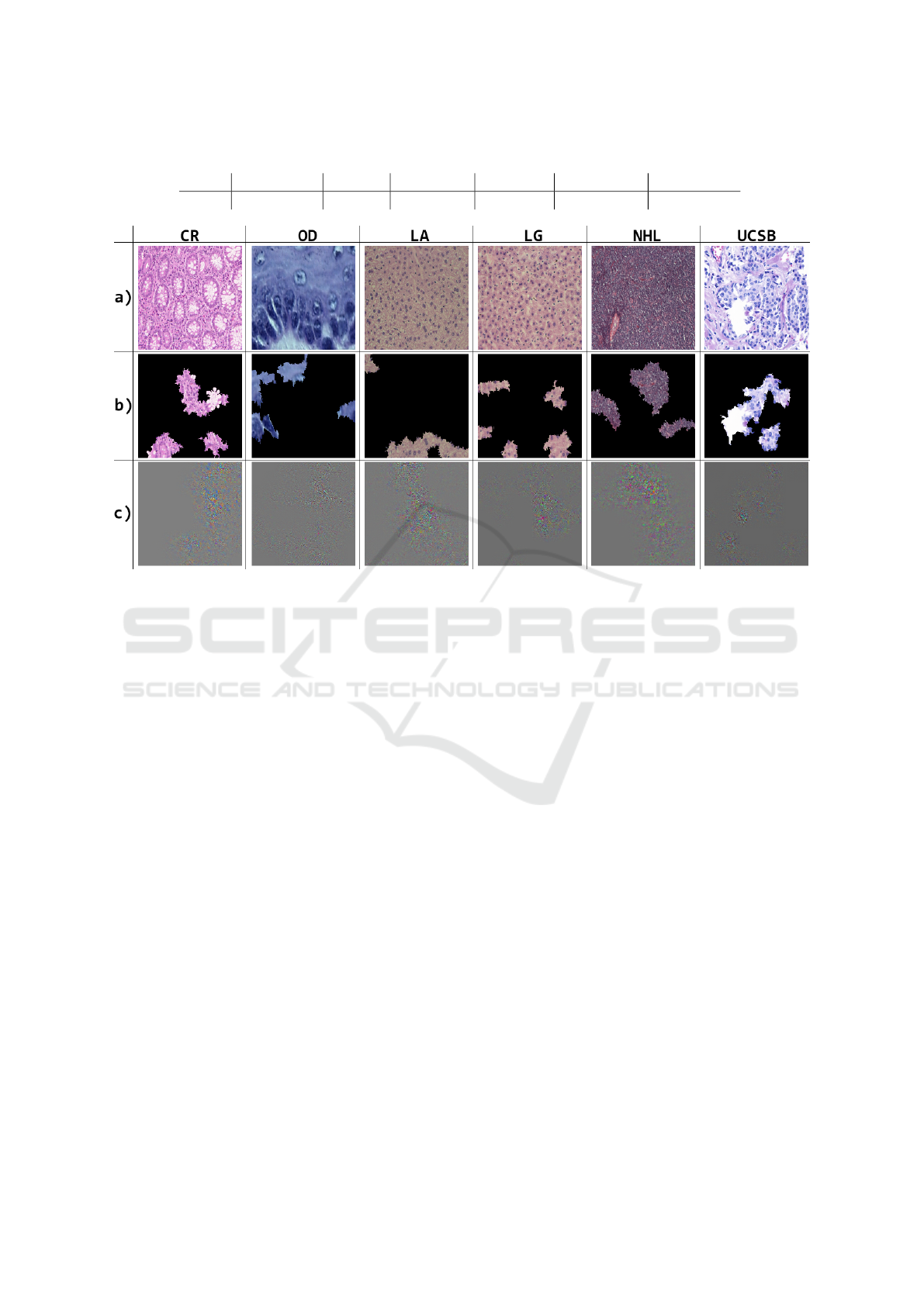
Table 1: Average accuracy of the tested models on the H&E histological image datasets used.

CNN GoogLeNet VGG16 ResNet-50 DenseNet EfﬁcientNet SqueezeNet

ACC 67% 99% 77% 69% 68% 91%

Figure 3: Examples of H&E histological image samples from each base and neural activation patterns, where: (a) original

images; (b) LIME results; (c) results via Guided Grad-CAM.

DF, LAC and PERC techniques available in (Ribeiro

et al., 2019) were applied to quantify the results pro-

vided by the LIME and Grad-CAM techniques. The

attributes obtained were used to compose feature vec-

tors representative of each type of image. Each vector

will be analysed using the strategies indicated in stage

The feature vectors obtained in stage 2 were anal-

ysed by applying a feature selection process in or-

der to reduce the dimensionality and identify the

best combination among the descriptors available

in each subset (Hsu et al., 2011; Mengdi et al.,

2018; Candelero et al., 2020). The process consisted

of ranking each entry using the ReliefF algorithm

(Robnik-Sikonja and Kononenko, 2003) and applying

a threshold to reduce the number of possible combi-

nations. The tested thresholds were deﬁned from the

10 best-ranked features, with increments of 10 fea-

tures (Ribeiro et al., 2019). The largest set was lim-

ited to 116 features, the maximum number of features

obtained at stage 2.

The discriminative power of each solution was ob-

tained by exploring eight classiﬁers obtained from

the Weka package (Frank et al., 2016): Random

Tree (RT), Random Forest (RaF), IBk, K*, Logit

Boost (LB), Rotation Forest (RoF), Simple Logistic

(SL) and Logistic (L). The evaluation process with

each classiﬁcation algorithm was carried out using

the cross-validation k-fold strategy, with k=10, and

metrics commonly available in the literature, such as

area under the ROC curve (AUC) and accuracy (Chiu,

2012). The GoogLeNet model was implemented in

the Python language, via the Pytorch library. The

Weka platform, version 3.8.5, was used to collect the

results of the accuracy and AUC measures from the

execution of stage 4. The proposal was carried out on

a notebook with a 2.4GHz Intel Core i5-9300H pro-

cessor, 8GB of RAM and a NVIDIA GeForce 1050

graphics card.

3 RESULTS

The proposed methodology was then applied to the set

of histological images, as described in section 2. The

best results were deﬁned by combining the classiﬁer

and the method for ranking the most relevant descrip-

tors, applying thresholds in the feature space. The

feature rankings were determined using the ReliefF

algorithm. Table 2 shows the highest average accu-

racy rates and AUC, with the total number of features

required to achieve the corresponding results on each

H&E dataset. Figure 4 shows a comparison between

the best average performance obtained by applying

the method using LIME and Guided Grad-CAM.

VISAPP 2024 - 19th International Conference on Computer Vision Theory and Applications

444

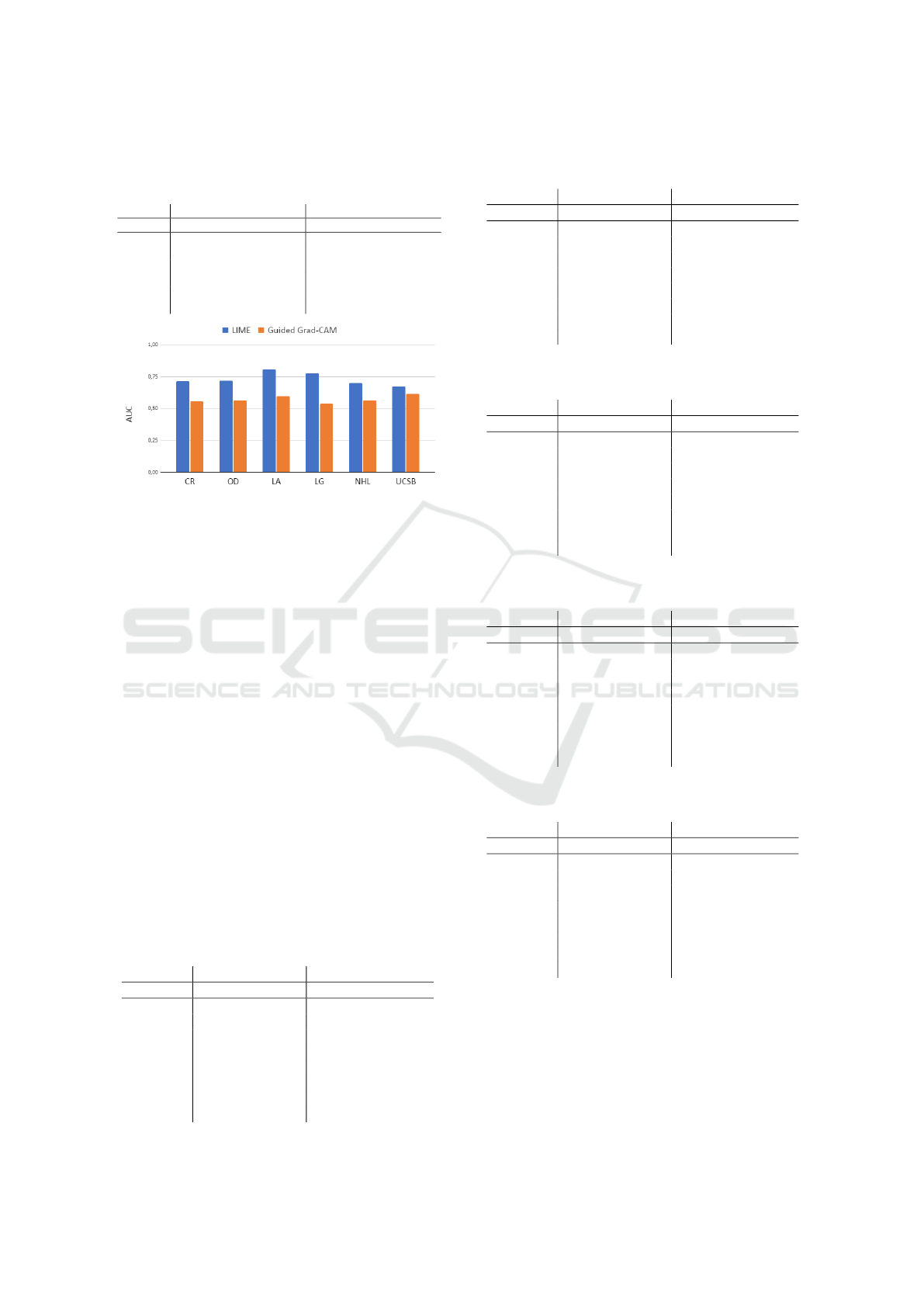
Table 2: Average performances obtained by applying the

proposed method, as well as an indication of the number of

features used (NoF) in each experiment.

LIME Guided Grad-CAM

Dataset AUC ACC NoF AUC ACC NoF

CR 0.714 66.74% 20 0.554 55.96% 110

DO 0.717 73.86% 20 0.562 69.22% 70

LA 0.804 60.80% 20 0.595 36.10% 70

LG 0.775 71.46% 30 0.535 54.76% 70

NHL 0.698 53.24% 40 0.560 38.60% 110

UCSB 0.672 63.15% 30 0.612 57.98% 10

Figure 4: Average AUC rates obtained from eight different

classiﬁers for each dataset.

From Figure 4, it can be seen that the LIME

method provided the best performance when com-

bined with fractal techniques to classify histological

H&E images. In all datasets, the best combinations

were obtained via LIME, with the highest average

AUC being provided by the LA dataset, using only

20 features.

Finally, to identify the classiﬁer that stood out in

each best result, Tables 3 to 8 show the AUC and ac-

curacy rates. The cases with the highest AUC have

been highlighted in bold. Note that the Logistic,

Simple Logistic, Rotation Forest and Random Forest

classiﬁers provided the highest AUC values, with the

highest value being 0.896 (30 features obtained via

LIME with the Logistic classiﬁer for the LG dataset).

In this case, the observed accuracy was 82.26%. For

this same dataset, the GoogLeNet model provided a

lower performance, with an AUC of 0.636 and an ac-

curacy of 62.26%, which allows us to verify the con-

tributions of our methodology in terms of classiﬁca-

tion.

Table 3: Results provided by each classiﬁer for the solution

with the highest average AUC for the CR dataset.

LIME Guided Grad-CAM

Classiﬁer AUC ACC AUC ACC

RT 0.605 61.21% 0.550 55.15%

RaF 0.752 69.09% 0.580 55.55%

IBk 0.559 58.18% 0.518 53.33%

K* 0.698 61.82% 0.611 61.21%

LB 0.774 69.09% 0.600 59.39%

RoF 0.768 72.12% 0.584 56.36%

SL 0.771 71.52% 0.504 54.55%

L 0.786 70.91% 0.486 52.12%

Table 4: Results provided by each classiﬁer for the solution

with the highest average AUC for the OD dataset.

LIME Guided Grad-CAM

Classiﬁer AUC ACC AUC ACC

RT 0.610 70.61% 0.556 65.88%

RaF 0.741 74.66% 0.587 70.61%

IBk 0.614 68.24% 0.500 63.18%

K* 0.657 68.92% 0.563 66.55%

LB 0.736 75.00% 0.547 69.26%

RoF 0.789 77.03% 0.645 76.01%

SL 0.798 79.05% 0.481 75.00%

L 0.788 77.36% 0.620 67.23%

Table 5: Results provided by each classiﬁer for the solution

with the highest average AUC for the LA dataset.

LIME Guided Grad-CAM

Classiﬁer AUC ACC AUC ACC

RT 0.672 51.52% 0.544 32.58%

RaF 0.840 63.64% 0.598 37.69%

IBk 0.726 60.42% 0.543 32.20%

K* 0.818 58.71% 0.549 32.00%

LB 0.779 54.55% 0.556 32.20%

RoF 0.875 67.80% 0.634 39.20%

SL 0.857 63.83% 0.651 40.72%

L 0.863 65.91% 0.684 42.23%

Table 6: Results provided by each classiﬁer for the solution

with the highest average AUC for the LG dataset.

LIME Guided Grad-CAM

Classiﬁer AUC ACC AUC ACC

RT 0.719 72.08% 0.547 56.23%

RaF 0.798 70.94% 0.517 54.34%

IBk 0.667 66.04% 0.526 52.83%

K* 0.731 64.91% 0.502 55.85%

LB 0.717 67.17% 0.459 52.45%

RoF 0.844 76.23% 0.577 56.98%

SL 0.829 72.08% 0.533 52.83%

L 0.896 82.26% 0.620 56.60%

Table 7: Results provided by each classiﬁer for the solution

with the highest average AUC for the NHL dataset.

LIME Guided Grad-CAM

Classiﬁer AUC ACC AUC ACC

RT 0.610 47.86% 0.533 37.70%

RaF 0.714 53.21% 0.610 41.18%

IBk 0.592 47.33% 0.545 39.04%

K* 0.631 44.65% 0.569 37.97%

LB 0.729 56.68% 0.526 36.36%

RoF 0.729 53.48% 0.582 41.18%

SL 0.771 59.36% 0.542 37.43%

L 0.807 63.37% 0.569 37.97%

To verify the relevance of the best solution ob-

tained with our proposal, the GoogLeNet model was

applied to the H&E histological image dataset to iden-

tify its discriminative capacity. Table 9 shows the best

results obtained via LIME and Grad-CAM, as well as

the performance obtained by the GoogLeNet network

when classifying the image datasets investigated here

Association of Grad-CAM, LIME and Multidimensional Fractal Techniques for the Classiﬁcation of H&E Images

445

Table 8: Results provided by each classiﬁer for the solution

with the highest average AUC for the UCSB dataset.

LIME Guided Grad-CAM

Classiﬁer AUC ACC AUC ACC

RT 0.605 60.34% 0.651 65.52%

RaF 0.736 68.97% 0.624 58.62%

IBk 0.691 67.24% 0.584 58.62%

K* 0.714 63.79% 0.627 55.17%

LB 0.653 63.79% 0.599 53.45%

RoF 0.644 55.17% 0.582 53.45%

SL 0.704 67.24% 0.591 53.45%

L 0.626 58.62% 0.641 65.52%

with the number of training epochs set to 30. Thus,

using Grad-CAM, a performance gain is observed in

four of the six datasets, with the highest gain being

17.67% for UCSB. On the other hand, the proposal

provided lower performance in the CR dataset, with

a difference of 22.16%. When the combinations are

made using LIME representations, the methodology

proved to be interesting as it indicated performance

gains in all datasets, with differences ranging from

0.08% to 40.24% in AUC rates. This indicates an-

other important contribution of this study, wherein the

combined use of fractal techniques, LIME representa-

tions and transfer learning can contribute to the foun-

dation of methods aimed at studying and recognising

patterns in the contexts investigated here of histologi-

cal H&E images.

Table 9: Performance rates (AUC) obtained with the model

and differences (Dif.) in each set of H&E images.

Dataset GoogLeNet LIME Grad-CAM

CR 0.785 0.786 0.611

DO 0.569 0.798 0.645

LA 0.612 0.875 0.684

LG 0.636 0.896 0.620

NHL 0.565 0.807 0.610

UCSB 0.536 0.736 0.651

4 CONCLUSION

In this paper. an approach involving the combined

use of XAI strategies to classify histological images

stained with Haematoxylin-Eosin (H&E) was pro-

posed. The neural activation patterns were obtained

from the GoogLeNet network. The feature vectors

were obtained by applying multiscale and multidi-

mensional fractal techniques. Each set of features was

evaluated using the ReliefF algorithm. The results

consisted of vectors with a reduced number of fea-

tures, which were tested by different classiﬁers. The

best combinations were then identiﬁed using LIME.

The results using the proposed method provided gains

in classiﬁcation rates, ranging from 0.08% to 40.24%.

The best combination occurred when using 30 fea-

tures with the Logistic classiﬁer, which provided an

AUC rate of 0.896 and an accuracy of 82.26% for

the LG dataset. In this same dataset, the GoogLeNet

network achieved a much lower performance than the

proposal, with an AUC of 0.636 and an accuracy of

62.26%. It is important to note that the best solu-

tion exploited a relevant set of features, using only

25.86% of the total descriptors available. This is an-

other important contribution of the proposed method,

as shown in the comparison with the metrics provided

by the GoogLeNet network. We believe that the main

contribution lies in providing detailed information on

combinations of techniques and feature subsets, as

well as an acceptable solution with few features.

For future work, we propose to study other CNN

models, include more feature selection algorithms

and explore other methodologies for extracting fea-

tures from the regions generated via Grad-CAM and

LIME. It would also be interesting to explore solu-

tions using a classiﬁer ensemble.

ACKNOWLEDGEMENTS

We thank the ﬁnancial support of Coordenac¸

de Aperfeic¸oamento de Pessoal de N

ıvel Su-

perior - Brasil (CAPES), the National Coun-

cil for Scientiﬁc and Technological Development

CNPq (Grants #132940/2019-1, #313643/2021-0 and

#311404/2021-9); the State of Minas Gerais Research

Foundation - FAPEMIG (Grant #APQ-00578-18); the

State of S

ao Paulo Research Foundation - FAPESP

(Grant #2022/03020-1) and the project NextGenAI

- Center for Responsible AI (2022-C05i0102-02),

supported by IAPMEI, and also by FCT plurianual

funding for 2020-2023 of LIACC (UIDB/00027/2020

UIDP/00027/2020.

REFERENCES

Adadi, A. and Berrada, M. (2018). Peeking inside the black-

box: A survey on explainable artiﬁcial intelligence

(xai). IEEE Access, PP:1–1.

Baish, J. W. and Jain, R. K. (2000). Fractals and cancer.

Cancer research, 60(14):3683–3688.

Candelero, D., Roberto, G. F., do Nascimento, M. Z.,

Rozendo, G. B., and Neves, L. A. (2020). Selec-

tion of cnn, haralick and fractal features based on evo-

lutionary algorithms for classiﬁcation of histological

images. In 2020 IEEE International Conference on

Bioinformatics and Biomedicine (BIBM), pages 2709–

2716. IEEE.

VISAPP 2024 - 19th International Conference on Computer Vision Theory and Applications

446

Chiu, D. (2012). Book review: ”pattern classiﬁcation”, r.

o. duda, p. e. hart and d. g. stork, second edition. In-

ternational Journal of Computational Intelligence and

Applications, 01.

Cruz-Roa, A., Caicedo, J. C., and Gonz

alez, F. A. (2011).

Visual pattern mining in histology image collec-

tions using bag of features. Artiﬁcial intelligence in

medicine, 52(2):91–106.

do Nascimento, M. Z., Martins, A. S., Azevedo Tosta, T. A.,

and Neves, L. A. (2018). Lymphoma images analysis

using morphological and non-morphological descrip-

tors for classiﬁcation. Computer Methods and Pro-

grams in Biomedicine, 163:65–77.

Doshi-Velez, F. and Kim, B. (2017). Towards a rigorous

science of interpretable machine learning.

Drelie Gelasca, E., Byun, J., Obara, B., and Manjunath, B.

(2008). Evaluation and benchmark for biological im-

age segmentation. In 2008 15th IEEE International

Conference on Image Processing, pages 1816–1819.

Frank, E., Hall, M. A., and Witten, I. H. (2016). The weka

workbench. online appendix for ”data mining: Practi-

cal machine learning tools and techniques”. Morgan

Kaufmann, Fourth Edition.

He, K., Zhang, X., Ren, S., and Sun, J. (2016). Deep resid-

ual learning for image recognition. In 2016 IEEE Con-

ference on Computer Vision and Pattern Recognition

(CVPR), pages 770–778.

Hsu, H., Hsieh, C. W., and Lu, M. (2011). Hybrid feature

selection by combining ﬁlters and wrappers. Expert

Systems with Applications, 38(7):8144–8150.

Iam Palatnik de Sousa, Marley Maria Bernardes Re-

buzzi Vellasco, E. C. d. S. (2019). Local inter-

pretable model-agnostic explanations for classiﬁca-

tion of lymph node metastases. Sensors (Basel,

Switzerland), 19, no. 13.

Ivanovici, M., Richard, N., and Decean, H. (2009a). Fractal

dimension and lacunarity of psoriatic lesions-a colour

approach. medicine, 6(4):7.

Ivanovici, M., Richard, N., and Decean, H. (2009b). Frac-

tal dimension and lacunarity of psoriatic lesions—a

colour approach—. Proceedings of the 2nd WSEAS

International Conference on Biomedical Electronics

and Biomedical Informatics, BEBI ’09, 6.

LeCun, Y., Bengio, Y., and Hinton, G. (2015). Deep learn-

ing. Nature, 521:436–44.

M. Sahini, M. S. (2014). Applications of percolation theory.

CRC Press.

Mahendran, A. and Vedaldi, A. (2016). Visualizing deep

convolutional neural networks using natural preim-

ages. International Journal of Computer Vision.

Mengdi, L., Liancheng, X., Jing, Y., and Jie, H. (2018).

A feature gene selection method based on relieff

and pso. In 2018 10th International Conference on

Measuring Technology and Mechatronics Automation

(ICMTMA), pages 298–301. IEEE.

o. A. AGEMAP, N. I. (2020). The atlas of gene expres-

sion in mouse aging project (agemap). Acesso em:

04/05/2020.

Rajaraman, S., Candemir, S., Kim, I., Thoma, G., and An-

tani, S. (2018). Visualization and interpretation of

convolutional neural network predictions in detecting

pneumonia in pediatric chest radiographs. Applied

Sciences, 8:1715.

Reyes, M., Meier, R., Pereira, S., Silva, C., Dahlweid,

M., Tengg-Kobligk, H., Summers, R., and Wiest, R.

(2020). On the interpretability of artiﬁcial intelligence

in radiology: Challenges and opportunities. Radiol-

ogy: Artiﬁcial Intelligence, 2:e190043.

Ribeiro, M. G., Neves, L. A., Nascimento, M. Z. d.,

Roberto, G. F., Martins, A. M., and Tosta, T. A. A.

(2019). Classiﬁcation of colorectal cancer based on

the association of multidimensional and multireso-

lution features. Expert Systems With Applications,

120:262––278.

Robnik-Sikonja, M. and Kononenko, I. (2003). Theoretical

and empirical analysis of relieff and rrelieff. Machine

Learning, 53:23–69.

Sahini, M. and Sahimi, M. (2014). Applications of percola-

tion theory. CRC Press.

Silva, A. B., Martins, A. S., Tosta, T. A. A., Neves, L. A.,

Servato, J. P. S., de Ara

ujo, M. S., de Faria, P. R., and

do Nascimento, M. Z. (2022). Computational analysis

of histological images from hematoxylin and eosin-

stained oral epithelial dysplasia tissue sections. Expert

Systems with Applications, 193:116456.

Sirinukunwattana, K., Pluim, J. P., Chen, H., Qi, X., Heng,

P.-A., Guo, Y. B., Wang, L. Y., Matuszewski, B. J.,

Bruni, E., Sanchez, U., et al. (2017). Gland segmen-

tation in colon histology images: The glas challenge

contest. Medical image analysis, 35:489–502.

Suman, R., Mall, R., Sukumaran, S., and Satpathy, M.

(2010). Extracting state models for blackbox software

components. Journal of Object Technology - JOT,

9:79–103.

Szegedy, C., Liu, W., Jia, Y., Sermanet, P., Reed, S.,

Anguelov, D., Erhan, D., Vanhoucke, V., and Rabi-

novich, A. (2015). Going deeper with convolutions.

In Proceedings of the IEEE conference on computer

vision and pattern recognition, pages 1–9.

Yosinski, J., Clune, J., Nguyen, A., Fuchs, T., and Lipson,

H. (2015). Understanding neural networks through

deep visualization.

Zerdoumi, S., Sabri, A. Q. M., Kamsin, A., Hashem, I.

A. T., Gani, A., Hakak, S., Al-Garadi, M. A., and

Chang, V. (2018). Image pattern recognition in big

data: taxonomy and open challenges: survey. Multi-

media Tools and Applications, 77(8):10091–10121.

Association of Grad-CAM, LIME and Multidimensional Fractal Techniques for the Classiﬁcation of H&E Images

447