Impute Water Temperature in the Swiss River Network Using LSTMs

Benjamin Fankhauser

1 a

, Vidushi Bigler

2 b

and Kaspar Riesen

1 c

Institute of Computer Science, University of Bern, Bern, Switzerland

Institute for Optimisation and Data Analysis, Bern University of Applied Sciences, Biel, Switzerland

Keywords:

Water Temperature Dataset, Imputing Missing Data, LSTM, Recurrent Neural Network, Time Series.

Abstract:

Switzerland is home to the sources of major European rivers. As the thermal regime of rivers is crucial for

the environment, the Federal Ofﬁce for the Environment has been collecting discharge and water temperature

data at 81 river water stations for several decades. However, despite diligent collection 30% of the water

temperature data is missing due to various reasons. These missing data are problematic in many ways – for

instance, in predicting water temperatures based on different models. To tackle this problem, we propose to

use LSTMs for water temperature imputing. In particular, we introduce three different scenarios – depending

on the available input data – to impute possible data gaps. Then, we propose several methods for each scenario.

For our empirical evaluation, we engineer a novel dataset (with ground truth) by artiﬁcially introducing gaps of

sizes 2, 10, 30 and 60 days in the middle of 90-day sequences. A rather simple interpolation baseline achieves

a competitive RMSE on gaps of two days. For larger gaps, however, this simple method clearly fails, and the

novel, far more sophisticated models signiﬁcantly outperform both interpolation and the current state of the

art in this application.

1 INTRODUCTION

The thermal regime of rivers is important for several

chemical and biological processes (Caissie, 2006).

Moreover, due to the complexity and dependence

of meteorological events, projections of future wa-

ter temperature is both crucial and challenging (Pic-

colroaz et al., 2016). Improving the performance of

predictive models is a crucial step of the overall sim-

ulation capabilities, especially when facing climate

change.

Switzerland has a ubiquitous landscape of wa-

ter bodies that consists of four major rivers (Rhine,

one, Inn, Ticino) with their corresponding tribu-

taries. In the high alpine regions there are glaciers,

snow ﬁelds and hydroelectric power plants. Within

the lowlands there is agriculture, a multitude of

medium and large cities as well as various lakes. All

this substantially inﬂuences the water network and es-

pecially the temperature of the water bodies.

For instance, if inﬂowing water stays for a long

time in a lake, the outﬂowing water corresponds to

the surface layer of the lake. This layer is more af-

https://orcid.org/0000-0002-7982-2669

https://orcid.org/0000-0001-6043-8264

https://orcid.org/0000-0002-9145-3157

fected by atmospheric exchange rather than the in-

ﬂowing water (the solar radiation is absorbed by par-

ticles in the water, then converted into heat and ﬁnally

exchanged with the water). Large cities (as a second

example of inﬂuence) can warm up on sunny days and

act as a boiler for rain water, which is then routed into

the nearest body of water.

Furthermore, we have other effects such as ground

water inﬂow or snow melt. Last but not least, on the

water surface there is a direct exchange with the sur-

rounding air. Hence, the water temperature is heav-

ily dependent on the air temperature. All in all, we

observe a fascinating network of water bodies with a

high complexity.

The present paper researches the important and

complex problem of water temperature imputation in

case of missing data. The topic of water tempera-

ture imputing has been approached with diverse mod-

els such as spatiotemporal varying coefﬁcients (Li

et al., 2017), or by remotely sensed Land Surface

Temperature (McNyset et al., 2015). In the present

paper we propose to combine Deep Learning with

the problem of imputing missing data in water tem-

perature sequences. To this end, we use Long short-

term Memory (LSTM) (Hochreiter and Schmidhuber,

1997) networks for data imputation. LSTMs have

732

Fankhauser, B., Bigler, V. and Riesen, K.

Impute Water Temperature in the Swiss River Network Using LSTMs.

DOI: 10.5220/0012358100003654

Paper published under CC license (CC BY-NC-ND 4.0)

In Proceedings of the 13th International Conference on Pattern Recognition Applications and Methods (ICPRAM 2024), pages 732-738

ISBN: 978-989-758-684-2; ISSN: 2184-4313

shown promising results in the related task of water

temperature prediction (Qiu et al., 2021; Jia et al.,

2021).

LSTMs are a special type of a recurrent neural net-

work (RNN) (Sherstinsky, 2020). An RNN in turn is a

neural network that is applied to a time series on every

time step. In addition to a standard RNN, an LSTM

keeps track of a hidden state and a memory state, two

vectors which are fed as inputs to the next time step

and will be altered by the LSTM.

This paper is a continuation of the work on the

Swiss River Network dataset where diverse open

challenges have been presented (Fankhauser et al.,

2023). In this previous publication, water tempera-

tures are predicted by means of LSTMs on the basis

of a graph based data structure. However, this predic-

tion is – at least in past – based on incomplete data.

We belief that improving data quality is an important

part for any water temperature prediction model (and

this is where the present work comes in).

The remainder of this paper is organized as fol-

lows. In Section 2, we describe the Swiss River Net-

work and its missing data in more detail. In Section 3,

we present several LSTM based methods to impute

missing water temperature data. The proposed mod-

els mainly differ in the amount of input variables they

actually use. These methods are then thoroughly eval-

uated in Section 4. Finally, we draw conclusions in

Section 5.

2 THE SWISS RIVER NETWORK

The Federal Ofﬁce of the Environment of Switzer-

land has been collecting water temperature and dis-

charge data for more than half a century. For bet-

ter monitoring of the climate change, about 30 addi-

tional water stations have been built during the period

of 2002 to 2010 (see Fig. 1 for an overview of the

Swiss River Network and the placement of the water

stations). In the context of this project, we have also

access to atmospheric measurements like the air tem-

perature which is provided by air stations (operated

by MeteoSwiss).

Recently, a graph structure has been introduced

which represents the connectivity of both water and

air stations (Fankhauser et al., 2023). The basic idea

is to use information from neighboring air stations

to make predictions for several target water stations.

In the present paper, we reuse this connectivity but

focus on the task of imputing missing data (rather

than pure water temperature predictions). Similar

to (Fankhauser et al., 2023) we work on temperatures

of daily averages and we do not use data prior to 1980

Figure 1: Overview of the Swiss River Network. Every blue

line is a body of water. 81 water stations measure the water

temperature and discharge (shown as black dots).

(due to the hydrological climate regime shift (Reid

et al., 2016; Woolway et al., 2017)).

2.1 Missing Data

Sensor failure, scheduled maintenance or problems

in the communication system are common causes for

missing data in real world applications. In our par-

ticular application, dirt can clog the tube where the

temperature sensor is placed in. Furthermore, tem-

perature sensors are affected by drift and have to be

calibrated regularly. A special case of missing data in

our case is the time before construction of the water

station: the water has been there but was not mea-

sured.

In our dataset we observe three types of missing

data.

• Gaps in air temperature data. In our dataset,

air temperature is nearly complete with only 1%

missing data.

• Gaps in discharge data: For discharge data, 6%

of the data is missing. Most water stations mea-

sured discharge before they were upgraded with a

temperature sensor.

• Gaps in water temperature data. Overall, 30% of

the data is missing.

In the present paper, we focus exclusively on the

third category of missing data.

For a more detailed analysis of the missing data in

the water temperature data, we show the frequencies

of different gap sizes with histograms (see Fig. 2).

We distinguish short gaps (up to 61 days), medium

gaps (from 62 to 729 days), and long gaps (730 days

or more). Short gaps are mostly due to unexpected

events, while long gaps, on the other hand, are more

likely due to operational decisions.

Regarding the histograms, it becomes clear that

the most common gap size is two days (with more

Impute Water Temperature in the Swiss River Network Using LSTMs

733

than 100 observations in total). Next, we observe sev-

eral gaps ranging from 30 days to 6000 days. Of in-

terest are ten gaps of exactly 365 days. Since they all

occur in the same year, we suspect an artiﬁcial rea-

son behind them. Furthermore, we observe relatively

many gaps, which are larger than 6,000 days. These

gaps correspond to the days before the construction

of the newer stations, which were put into operation

between 2002 and 2010.

3 METHODS FOR IMPUTING

MISSING DATA

In this section, we present seven methods to impute

missing water temperature data on the Swiss River

Network. The methods are grouped by the number of

input variables they have available (resulting in three

groups). Each of the three groups represents a differ-

ent scenario.

1. In the ﬁrst scenario, we assume to have access to

the water temperature of the target station only

(i.e. the station with the gap). Water temperature

data is available before and after the gap.

2. In the second scenario, we assume to have ad-

ditionally access to air temperature data dur-

ing the gap to use traditional models like

Air2Stream (Toffolon and Piccolroaz, 2015).

3. In the third scenario, we assume to have access to

all available input variables. Namely, we use the

discharge data as well as the graph structure of the

Swiss River Network to obtain water temperature

measurements of neighboring stations.

The left side of Fig. 3 illustrates the three scenarios

and in particular, which data the scenarios have at

their disposal.

Before describing the individual methods of the

three scenarios in more detail (in Sections 3.2, 3.3,

and 3.4) we brieﬂy describe the generalized architec-

ture of the underlying model.

3.1 General Architecture

The available data is split into a part before the gap,

auxiliary variables during the gap and a part after the

gap. In general, each of the three parts are inputted

to their own LSTM and then combined together. The

LSTM working on auxiliary variables is used for esti-

mating the values in the gap and thus called the main

network. The right side of Fig. 3 shows the three pos-

sible LSTMs.

If a certain model has a ”Pr” in its identiﬁer it

uses an LSTM to encode the water temperature be-

fore the gap as initial state for the main network. The

main network estimates the missing values of the gap.

Its input depends on the scenario and is also imple-

mented as an LSTM. If the data after the gap is used as

well we add an additional LSTM and convert the main

network into a bidirectional conﬁguration (in this case

the identiﬁer of the model contains a ”Po”).

Note, however, that only two methods stemming

from the ﬁrst scenario make use of the water tem-

perature data after the gap (since they have the least

amount of information available). In theory, every

method with the Pr-LSTM could be extended to the

bidirectional setting to make use of the data after the

gap. Yet, we focus on the unidirectional way for

our methods as this allows the methods to ﬁll gaps

where only one side of the temporal direction is avail-

able, namely estimates in future or before construc-

tion time.

3.2 Scenario 1: Water Temperature

Based Methods

The ﬁrst group of methods has only access to the wa-

ter temperature of the target station before and after

the gap. We propose three methods.

Interpolation. The ﬁrst method consists of a simple

linear interpolation, i.e. the convex combination of the

temperature of the last day before and the ﬁrst day

after the gap.

Pr2Gap. The second method is termed Pr2Gap and

trains an LSTM on the water temperature before the

gap in order to predict the missing values in the gap.

During the gap, the LSTM is invoked and predicts

each day of the gap as a day in future. Note that this

method does not make use of the water temperature

after the gap.

PrPo2Gap. The third method is termed PrPo2Gap

and can be seen as an extension of the second method

in a bidirectional conﬁguration. It uses an LSTM on

the water temperature before the gap and a second

LSTM on the water temperature after the gap in op-

posite direction.

3.3 Scenario 2: Air Temperature Based

Methods

In many real world scenarios, we have access to data

of a near by air temperature station during the gap.

Hence, the second group of methods has – in theory –

access to the water temperature before and after the

gap, as well as to neighboring air temperature sta-

tions. We propose two different methods (note that

ICPRAM 2024 - 13th International Conference on Pattern Recognition Applications and Methods

734

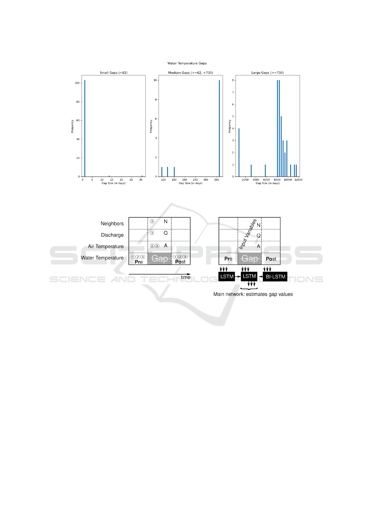
Figure 2: The distribution of gaps of different length in the water temperature data from 1980 to 2021 of the Swiss River

Network. We observe that small gaps occur more frequently, but gaps of the medium and large category contribute much

more to the overall 30% of missing data.

Figure 3: Overview of the three scenarios: On the left we see the data around the gap. Scenario 1 only uses water temperature

from before and after the gap. Scenario 2 has additionally access to the air temperature during the gap and Scenario 3 might

use all available data (i.e. additionally data from neighboring stations and discharge data). To the right we have the generalized

architecture of the seven methods.

the identiﬁers of these methods now include the ab-

breviation A for air temperature).

A2Gap. The ﬁrst method is termed A2Gap and mod-

els the air to water temperature relationship in the

same way as Air2Stream (Toffolon and Piccolroaz,

2015) or corresponding LSTM versions (Qiu et al.,

2021). The model uses the air temperature during the

gap to estimate each day of the gap individually. No

water temperature is taken into account (neither be-

fore nor after the gap), making this model indepen-

dent of the gap size.

PrA2Gap. The second method is termed PrA2Gap

and is similar to the A2Gap method but adds an ad-

ditional LSTM to encode the previous water temper-

ature. This encoded state is then fed to the A2Gap

model as ﬁrst initial state in order to make use of the

available water temperature before the gap.

3.4 Scenario 3: Neighbor Based

Methods

In this third scenario, we make use of all available

data of the Swiss River Network. Additional to the

previous two scenarios, we add discharge and use the

Swiss River Network to determine neighboring sta-

tions. In particular, we use the water temperature of

neighboring stations as input and refer to it as neigh-

bor temperature. Note that the abbreviations of these

methods now include a Q (for discharge) and an N

(for neighbor temperature).

AQN2Gap. The ﬁrst method of this group is the ex-

tension of the A2Gap method but uses more input

variables. In particular, it has access to the air tem-

perature, discharge and neighbor temperature during

Impute Water Temperature in the Swiss River Network Using LSTMs

735

the gap. However, this method does not use water

temperature before or after the gap.

PrAQN2Gap. The second method of this group uses

an additional LSTM to encode the water temperature

before the gap. This encoded state is then used as

initial state for the main network.

FCN-AQN2Gap. The third method is employed to

compare the LSTM performance against a fully con-

nected neural network (FCN). As we will use gaps

of ﬁxed size in our experiment, we can train an FCN

ﬁtting precisely the size of the gap and thus replace

the LSTM of the main network with an FCN. It uses

the same input data as the AQN2Gap model. This

means it only relies on auxiliary variables during the

gap. This method is interesting in practice as a trained

FCN-AQN2Gap model for a gap size of k

′

can be used

to ﬁll any gap of size k as long as k ≤ k

′

. Moreover,

a gap of size 2k can be interpreted as two consecutive

gaps of size k.

4 EXPERIMENTAL EVALUATION

4.1 Experimental Setup

As we do not have ground truth values for the actual

gaps in the water temperature time series, we simulate

artiﬁcial gaps in our experiment. To this end, we se-

lect gap-free sequences of 90 days and artiﬁcially in-

troduce water temperature gaps in the middle of each

sequence. In total, we select 412,436 sequences from

55 water stations for our evaluation. The sequences

overlap in time. The inserted gaps are of length 2, 10,

30, and 60 days. We split the resulting sequences into

disjoint sets for training, validation and testing (64%,

16% and 20% of the data, respectively). For each pair

of method and station, we run a grid search over width

and depth of the networks and the learning rate. The

validation set is used to determine the best hyperpa-

rameters. The presented results are obtained on the

untouched test set sequences.

For quantitative comparison we use the root mean

square error (RMSE), formally deﬁned by

RMSE =

∑

i=1

− ˆy

)

, (1)

where y

is the ground truth value at the i-th position

in the gap and ˆy

is the value estimated by the model.

Obviously, the lower the RMSE the better the model.

Our code will be made publicly available for re-

search purpose on the Git Repository of our research

group

https://github.com/Pattern-Recognition-Group-

4.2 Results and Discussion

For each method and water station we report the

RMSE of the best model on the untouched test set.

This results in 55 data points per method. Fig. 4

shows the results as box-plots diagram for all four gap

sizes (2, 10, 30, and 60 days). In particular, the box-

plots show the median RMSE for all eight methods

with a horizontal line, the interquartile range (IQR),

and the whiskers pointing to the smallest and largest

elements still within 1.5 times the IQR (we also show

possible outliers with circles).

For a gap size of two days, the results of linear in-

terpolation are compatible to the best models. How-

ever, with larger gaps the performance of this rather

simple method substantially deteriorates. The same

holds for the other two methods of the ﬁrst scenario.

The methods based on other auxiliary variables,

which are accessible during the gap, namely air tem-

perature, discharge and neighboring water tempera-

ture, maintain a constant performance independent of

the size of the actual gap. The only exception is the

FCN based method, which deteriorates slightly with

increasing gap size.

Adding neighboring water temperatures and dis-

charge as input to the model, outperforms more tradi-

tional methods solely based on air temperature. The

Pr-based variants, which encode the available wa-

ter temperatures before the gap, constantly improve

their counterparts that have no access to this infor-

mation. Replacing the main network LSTM of the

AQN2Gap model with a fully connected neural net-

work decreases performance in our experimental set-

ting.

The worst model is Pr2Gap, which performs

poorly on all gap sizes and generally has the largest

RMSE. Vice versa, we can report that on all tested

gap sizes the PrAQN2Gap model achieves the best

performance. This particular model is based on all

available data (air and discharge data as well as water

temperature of the neighboring stations) and achieves

an RMSE of 0.47, 0.52, 0.54, and 0.55 on the data

with gaps of 2, 10, 30, and 60 days, respectively.

5 CONCLUSIONS

After revisiting the hydrological data of the Swiss

River Network (Fankhauser et al., 2023), we ﬁnd that

this real world application suffers from missing data

(up to 30% of the data). Ignoring these gaps in the

data is an unsatisfactory solution for both practition-

UniBe/swiss-river-network

ICPRAM 2024 - 13th International Conference on Pattern Recognition Applications and Methods

736

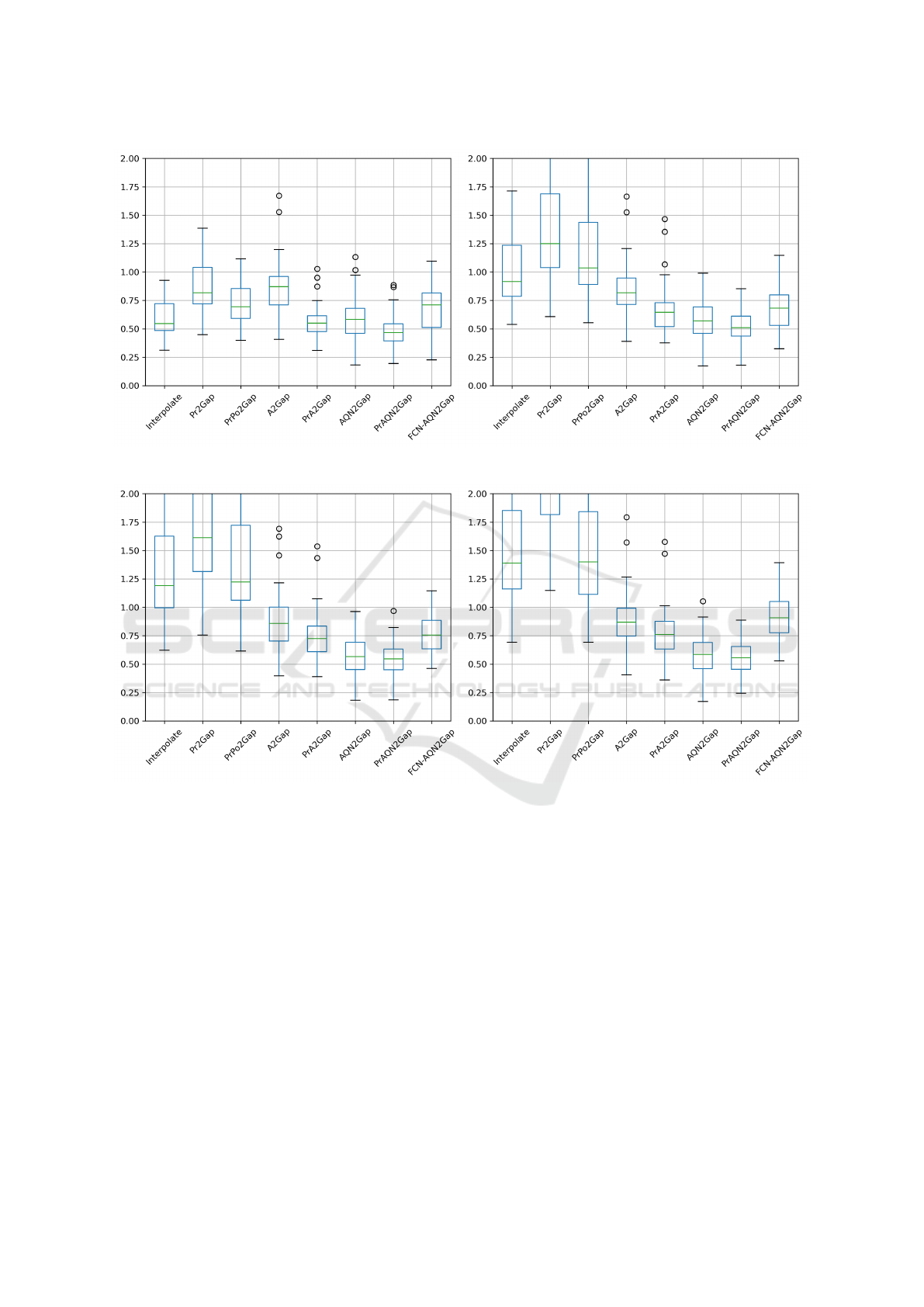
(a) Gap size 2. (b) Gap size 10.

Figure 4: Results of the experimental evaluation. Reported is the RMSE on the untouched test set sequences. The scale is cut

off at a value of 2 in order to not distort the visual comparison.

ers as well as data analysts. For this reason, we ad-

dress the task of data imputation in this paper.

We assume three different scenarios that could oc-

cur in real-world applications. That is, depending on

the circumstances of the gap, one of the three intro-

duced scenarios might occur. For each scenario differ-

ent model architectures are proposed and researched.

The different models differ primarily to the extent that

they make use of different data (such as water temper-

ature data before the gap or air temperatures or water

temperatures of neighboring stations during the gap).

In order to evaluate the methods we run an exper-

iment on a novel dataset with artiﬁcially created gaps

of different sizes (2, 10, 30, and 60 days). The maxi-

mal gap size is rather small, but the stable results and

constructions independent of the gap size allow us to

extend our conclusions to larger gap sizes. In partic-

ular as some of the proposed techniques, viz. A2Gap,

AQN2Gap, FCN-AQN2Gap, give consistently good

results irrespective of the gap size.

Considering the results obtained, we can draw the

following three main conclusions.

1. For small gaps of two days the interpolation

method is performing well in respect of its sim-

plicity, and we can recommend to use it.

2. For any gap size larger than ten days, however,

more sophisticated models are necessary. The

Impute Water Temperature in the Swiss River Network Using LSTMs

737

model PrAQN2Gap performs the best in general.

With an average RMSE close to 0.55 it outper-

forms current state of the art methods which are

based solely on air temperature. To be fair, their

experimental setup is slightly different and we in-

troduce the A2Gap method as representable com-

petitor.

3. In an ablation experiment, we replace the LSTM

of the main network with a fully connected net-

work. As the results of this particular model de-

teriorates with increasing gap size, we conclude

that LSTMs seems to be beneﬁcial for our task.

In future work we plan to impute missing data in

discharge data and research the impact of the artiﬁ-

cially created gap free dataset on water temperature

prediction models. Another direction of work is to

retrospectively investigate the measured data to ﬁnd

undetected outliers.

ACKNOWLEDGEMENTS

This project is supported by the Swiss National

Science Foundation (SNSF) Grant Nr. PT00P2

206252. Data are kindly provided by the

Federal Ofﬁce for the Environment and Me-

teoSwiss. Calculations were performed on UBELIX

(https://www.id.unibe.ch/hpc), the HPC cluster at the

University of Bern.

REFERENCES

Caissie, D. (2006). The thermal regime of rivers: a review.

Freshwater biology, 51(8):1389–1406.

Fankhauser, B., Bigler, V., and Riesen, K. (2023). Graph-

based deep learning on the swiss river network.

In International Workshop on Graph-Based Repre-

sentations in Pattern Recognition, pages 172–181.

Springer.

Hochreiter, S. and Schmidhuber, J. (1997). Long short-term

memory. Neural computation, 9(8):1735–1780.

Jia, X., Zwart, J., Sadler, J., Appling, A., Oliver, S., Mark-

strom, S., Willard, J., Xu, S., Steinbach, M., Read,

J., et al. (2021). Physics-guided recurrent graph

model for predicting ﬂow and temperature in river net-

works. In Proceedings of the 2021 SIAM International

Conference on Data Mining (SDM), pages 612–620.

SIAM.

Li, H., Deng, X., and Smith, E. (2017). Missing data im-

putation for paired stream and air temperature sensor

data. Environmetrics, 28(1):e2426.

McNyset, K. M., Volk, C. J., and Jordan, C. E. (2015). De-

veloping an effective model for predicting spatially

and temporally continuous stream temperatures from

remotely sensed land surface temperatures. Water,

7(12):6827–6846.

Piccolroaz, S., Calamita, E., Majone, B., Gallice, A.,

Siviglia, A., and Toffolon, M. (2016). Prediction of

river water temperature: a comparison between a new

family of hybrid models and statistical approaches.

Hydrological Processes, 30(21):3901–3917.

Qiu, R., Wang, Y., Rhoads, B., Wang, D., Qiu, W., Tao, Y.,

and Wu, J. (2021). River water temperature forecast-

ing using a deep learning method. Journal of Hydrol-

ogy, 595:126016.

Reid, P. C., Hari, R. E., Beaugrand, G., Livingstone, D. M.,

Marty, C., Straile, D., Barichivich, J., Goberville, E.,

Adrian, R., Aono, Y., et al. (2016). Global impacts

of the 1980s regime shift. Global change biology,

22(2):682–703.

Sherstinsky, A. (2020). Fundamentals of recurrent

neural network (rnn) and long short-term memory

(lstm) network. Physica D: Nonlinear Phenomena,

404:132306.

Toffolon, M. and Piccolroaz, S. (2015). A hybrid model for

river water temperature as a function of air tempera-

ture and discharge. Environmental Research Letters,

10(11):114011.

Woolway, R. I., Dokulil, M. T., Marszelewski, W., Schmid,

M., Bouffard, D., and Merchant, C. J. (2017). Warm-

ing of central european lakes and their response to

the 1980s climate regime shift. Climatic Change,

142:505–520.

ICPRAM 2024 - 13th International Conference on Pattern Recognition Applications and Methods

738