Pre-Training and Fine-Tuning Attention Based Encoder Decoder

Improves Sea Surface Height Multi-Variate Inpainting

eo Archambault*

1,2 a

, Arthur Filoche

1,3 b

, Anastase Charantonis

4,5 c

and Dominique B

eziat

1 d

Sorbonne Universit

e, CNRS, LIP6, Paris, France

Sorbonne Universit

e, LOCEAN, Paris, France

UWA, Perth, Australia

ENSIIE, LaMME, Evry, France

Inria, Paris, France

Keywords:

Image Inverse Problems, Deep Neural Network, Spatiotemporal Inpainting, Multi-Variate Observations,

Transfer Learning, Satellite Remote Sensing.

Abstract:

The ocean is observed through satellites measuring physical data of various natures. Among them, Sea Surface

Height (SSH) and Sea Surface Temperature (SST) are physically linked data involving different remote sensing

technologies and therefore different image inverse problems. In this work, we propose to use an Attention-

based Encoder-Decoder to perform the inpainting of the SSH, using the SST as contextual information. We

propose to pre-train this neural network on a realistic twin experiment of the observing system and to ﬁne-tune

it in an unsupervised manner on real-world observations. We show the interest of this strategy by comparing

it to existing methods. Our training methodology achieves state-of-the-art performances, and we report a

decrease of 25% in error compared to the most widely used interpolations product.

1 INTRODUCTION

In the past decades, satellite remote sensing pro-

duced an unprecedented amount of data, which led

to a deeper understanding of the Earth system. For

instance, out of the 50 essential climate variables

deﬁned by the Global Climate Observing System

(GCOS) 26 are estimated through satellite (Yang

et al., 2013). In the ﬁeld of oceanography, satellites

are used to measure various ocean surface variables,

such as height, temperature, ice fraction, or chloro-

phyll concentration. The nature of sea-surface satel-

lite observations requires solving various image in-

verse problems, such as inpainting, super-resolution,

denoising, etc.

In this study, we focus on the inpainting of the

Sea Surface Height (SSH), which is a very important

variable of the ocean state, as it is used to retrieve sur-

face currents through the geostrophic approximation.

The altimeters embarked in satellites measure their

https://orcid.org/0000-0001-8051-0534

https://orcid.org/0000-0001-7779-6105

https://orcid.org/0000-0003-4953-2684

https://orcid.org/0000-0003-1444-8212

distance to the sea surface through the return time of

a radar pulse. Because of this technique, the nadir-

pointing altimeters sensors are only able to take mea-

sures vertically, along their ground tracks (Martin,

2014). Therefore, producing a fully grided map of the

SSH is a challenging spatiotemporal inpainting prob-

lem. It is currently tackled by the Data Uniﬁcation

and Altimeter Combination System, DUACS, (Taburet

et al., 2019) which is a linear optimal interpolation of

the along-track data from several satellites (Brether-

ton et al., 1976). However, prior works show that

DUACS produces overly smooth maps, and is miss-

ing a lot of small structures and eddies (Amores et al.,

2018; Stegner et al., 2021). To enhance the quality

of this reconstruction, we are interested in exploiting

contextual variables physically related to SSH, and

with a similar or ﬁner resolution. Among different

possibilities, Sea Surface Temperature (SST) is linked

to surface currents, as the heat is passively transported

by oceanic circulation, and is acquired through direct

infrared measures leading to images with higher spa-

tiotemporal sampling.

In the last years, deep learning has emerged as one

of the leading methods to solve image inverse prob-

100

Archambault, T., Filoche, A., Charantonis, A. and Béréziat, D.

Pre-Training and Fine-Tuning Attention Based Encoder Decoder Improves Sea Surface Height Multi-Variate Inpainting.

DOI: 10.5220/0012357400003660

Paper published under CC license (CC BY-NC-ND 4.0)

In Proceedings of the 19th International Joint Conference on Computer Vision, Imaging and Computer Graphics Theory and Applications (VISIGRAPP 2024) - Volume 3: VISAPP, pages

100-109

ISBN: 978-989-758-679-8; ISSN: 2184-4321

lems (McCann et al., 2017) and speciﬁcally inpainting

problems (Jam et al., 2021; Qin et al., 2021). Their

ﬂexibility allows neural networks to include contex-

tual information such as SST, and several studies con-

clude that using it in a multi-variate neural network

leads to a signiﬁcant improvement of the SSH recon-

struction (Nardelli et al., 2022; Fablet et al., 2023;

Thiria et al., 2023; Martin et al., 2023; Archambault

et al., 2023). However, training neural networks usu-

ally requires pairs of ground truth and observations

which we lack in real-world situations. To overcome

this limitation, previous works have examined two

main strategies: training the network on a realist sim-

ulation of the observing system (Fablet et al., 2023)

or using loss functions not requiring ground truth (Ar-

chambault. et al., 2023; Martin et al., 2023; Archam-

bault et al., 2023). As the ﬁrst method entirely relies

on the realism of the twin experiment its application

to real-world observations suffers from a domain gap,

especially for multi-variate approaches. To this day,

if the feasibility of training SSH-only networks on

simulation alone has been demonstrated to be possi-

ble (Fablet et al., 2023), transferring multi-variate ap-

proaches has never been successfully performed. On

the other hand, our previous work (Archambault et al.,

2023) shows that the method trained using only obser-

vations suffers from a drop in performance compared

to fully supervised ones.

In this work, we are interested in combining the

advantages of these two methods. We propose to per-

form a pre-training on a multi-variate simulation of

the observing system, and a ﬁne-tuning using only

real-world observations. This paper is structured as

follows: ﬁrst, we introduce the different data used

in this study and present the inpainting methods.

Then we compare the different learning strategies and

present a benchmark of this application.

2 DATA

2.1 Observing System Simulation

Experiment

In geosciences, one of the major difﬁculties is that the

ground truth we aim to estimate is often inaccessi-

ble. To understand the impact of observation systems

on the reconstruction process, researchers employ a

method known as the Observing System Simulation

Experiment (OSSE). This technique involves simu-

lating the observation operator on a physical simula-

tion, in our case to replicate realistic satellite measure-

ments. The oceanographic community widely uses

it as it provides ways to test reconstruction methods

and errors (Amores et al., 2018; Stegner et al., 2021;

Gaultier et al., 2016). In this context, we use the

SSH and SST variables from a realistic simulation

as the ground truth upon which we simulate satellite

measures. In this study, we select a portion of the

North Atlantic Ocean (from latitudes 33° to 43° and

longitudes -65° to -55°) of the Global Ocean Physi-

cal Reanalysis, GLORYS (CMEMS, 2020). We re-

trieve 7194 daily images of data starting from Mars

20, 2000 to December 29, 2019. Hereafter, we call X

the ground truth variable, H our simulated observing

operator, and Y = H (X) their associated simulated

observations. Following our previous work (Archam-

bault et al., 2023), we present a multivariate OSSE

with enough pairs of observations and ground truth to

train a neural network.

2.1.1 Sea Surface Height

The nadir-pointing SSH observations are localized on

a precise spatiotemporal support (denoted Ω) which

we want to reproduce in our OSSE. Using the support

from the Copernicus sea level real-world observa-

tions (CMEMS, 2021), and the ground truth data X

ssh

from GLORYS we simulate SSH observations Y

ssh

the trilinear interpolation of X

ssh

on each point of the

support. We add an instrumental error ε ∼ N (0, σ)

with σ = 1.9cm, which is the distribution used in the

Ocean data challenge 2020 (CLS/MEOM, 2020). The

SSH observing system is thus deﬁned as follows:

ssh

= H

ssh



ssh

, Ω



+ ε (1)

where H

ssh

SSH observation operator. An example

of these simulated along-track measurements is pre-

sented in Figure 1.

2.1.2 Sea Surface Temperature

SST remote sensing relies on direct infrared measure-

ments, enabling broader coverage but making the data

susceptible to cloud interference. To address gaps left

by the clouds, the oceanographic community merges

the images taken by several satellites through linear

interpolation. The interpolated images present artiﬁ-

cially smoothed structures in thick cloud regions. We

simulate this process as follows:

sst

= H

sst



sst



(2)

= (1 − C) ⊙



sst

+ ε



+C ⊙ G

⋆



sst

+ ε



where ⊙ is the element-wise product, ⋆ the convo-

lution product, ε is a white Gaussian noise image of

size 32 × 32 linearly upsampled to a 128× 128 image,

and C is the cloud cover (1 when a cloud is present

and 0 elsewhere). We ﬁrst add ε to the SST ground

Pre-Training and Fine-Tuning Attention Based Encoder Decoder Improves Sea Surface Height Multi-Variate Inpainting

101

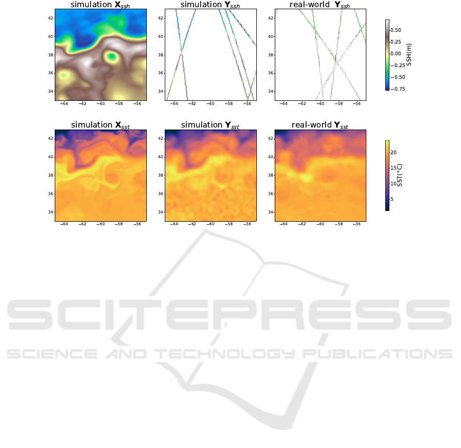
Figure 1: Daily example of SSH and SST data. The ﬁrst column is the ground truth from the physical model, the second

column is our simulation of the observations, and the last is the real-world satellite data.

truth to simulate the instrumental error, and then per-

form a Gaussian blur with a kernel G

(σ = 16km).

This smoothing is then applied only when clouds are

present, to mimic in-equal spatial resolution of the

satellite SST images. H

sst

adds a noise with a stan-

dard deviation of 0.5°C out of the 4.96°C of the SST

standard deviation.

2.2 Real-World Data

For SSH real-world data we propose to use the

ungrided data used as inputs of the DUACS pro-

tocol (CMEMS, 2021). Concerning SST data,

we use the Multiscale Ultrahigh Resolution (MUR)

SST (NASA/JPL, 2019). These products in cloud-

free, as missing values are inpainted using a linear

optimal interpolation, which leads to a smoothing of

high spatial frequencies when could are present.

3 PROPOSED METHOD

To exploit the temporal coherence of the sparsely ob-

served ocean structures, we propose to perform the

SSH inpainting on a time series of 21 daily images.

The neural network f

estimates the SSH ﬁelds

ssh

from observations Y, which could be Y

ssh

for SST-

agnostic networks or (Y

ssh

, Y

sst

) for SST-aware net-

works. Y

ssh

, Y

sst

ssh

have the same size (21 images

of size 128 by 128).

3.1 Architecture

Following our previous work (Archambault et al.,

2023) we propose to use an Attention Based Encoder

Decoder (ABED) to perform the inpainting. The ar-

chitecture of the network is presented in Figure 2. It

starts with two encoding blocks that divide the spatial

dimensions of the images by 2. Then spatiotemporal

attention and decoding blocks are performed succes-

sively to get back to the original size. This mechanism

allows the network to highlight essential features in

the input images such as oceanic eddies, while reduc-

ing the importance of irrelevant ones such as cloudy

areas for instance. Attention modules are widely used

in many computer vision tasks including image in-

painting (Guo et al., 2021) and can be transposed to

geoscience applications (Che et al., 2022; Archam-

bault et al., 2023). Furthermore, the nature of atten-

tion modules is well suited to ﬁne-tuning as irrelevant

pre-trained ﬁlters can easily be weighed with small

values during the reﬁtting of attention layers.

Our spatiotemporal attention block is divided into

two steps: temporal and spatial attention. Our ap-

proach follows the Convolutional Block Attention

Module (CBAM) principle introduced by (Woo et al.,

2018), which proposed to compute consecutively

channel and spatial attention. We adapt this concept

to spatiotemporal data by integrating temporal infor-

mation into the channel attention mechanism. The

temporal attention begins by computing the spatial

average for each channel and instant, resulting in a

tensor of dimensions C × T , where C denotes the

VISAPP 2024 - 19th International Conference on Computer Vision Theory and Applications

102

Encoder block

Decoder block

Attention Based Encoder Decoder

MLP

Spatial

attention

Temporal

attention

Attention block

Conv3D

Batchnorm

ReLU

Maxpool

Bilinear

upsampling

Spatial

Average

Residual

addition

Hadamard

product

Sigmoid

Figure 2: Overview of the Attention-Based-Encoder-

Decoder. The network starts with two encoding blocks each

dividing the spatial dimensions of the images by 2. Atten-

tions modules are then performed, followed by a residual

connection and a decoding block.

number of channels and T represents the length of

the time series. We then apply a two-layer perceptron

with shared weights across all time steps followed by

a sigmoid activation. The resulting tensor has values

between 0 and 1 and we multiply it to the input ten-

sor to perform temporal attention. To proceed with

spatial attention, we use a 3-dimensional convolution,

where the kernel’s temporal size equals the length of

the time series. We also use a sigmoid activation to

obtain a 2D image between 0 and 1 before multiply-

ing with the input tensor. Subsequently, a residual

skip connection is computed. This described block is

iteratively applied 4 times for the ﬁrst block, 2 times

for the second block, and once for the ﬁnal block as

Figure 2 shows

Our implementation and training data are available

here: https://gitlab.lip6.fr/archambault/visapp2024

3.2 Loss Functions

We propose two loss functions to train this neural net-

work. The ﬁrst method takes the Mean Square Er-

ror (MSE) on the entire image in a supervised fash-

ion. This is applicable exclusively in the OSSE setting

where we have access to the ground truth during train-

ing. The second approach uses an unsupervised loss

function, enabling training in scenarios where only

observations are accessible. Figure 3 gives a visual

overview of the two training methods.

We detail hereafter the unsupervised loss function.

Prior studies suggest that it is possible to perform the

SSH interpolation from observations only. Using a

spatiotemporal Deep Image Prior strategy (Ulyanov

et al., 2017), meaning overﬁting observations from a

white noise, (Filoche et al., 2022) showed that if cho-

sen correctly, the architecture of the neural network

acts as a regularization that outperforms DUACS. Fol-

lowing the same principle (Archambault. et al., 2023)

estimated an SSH map from gridded SST images on

one year of data. One of the major limitations of these

two methods is that they need to be reﬁtted if ap-

plied to unseen data which makes them extremely in-

efﬁcient computationally speaking. To overcome this

limitation, (Archambault et al., 2023; Martin et al.,

2023) proposed to train the neural network in a way

that doesn’t require reﬁtting and that enables the use

of contextual information such as SST.

To train the neural network in a context where

only observations are available, we apply the ob-

serving operator H

ssh

on the estimate ﬁeld

ssh

) before computing the MSE. This allows us

to get back to the observation domain where we have

data to constrain the method. The unsupervised loss

function is deﬁned as follows:

unsup

ssh

) =

∑



ssh

− H

ssh

(

ssh

)



∑



ssh

−

ssh



(3)

N is the number of SSH samples in the observation

vector Y

ssh

and

ssh

is the estimation of the obser-

vations. To ensure that the network produces a valid

estimation outside of the SSH measures given as in-

puts, we leave aside the data from one satellite (out of

three to six satellites depending on the period) from

the neural network’s inputs. In Figure 3 we call this

input vector Y

ssh

. The network is then controlled on

all the observations, the ones given in input and the

left-aside. Therefore, to accurately estimate the with-

held observations, the network is forced to generalize

well on the whole image.

Pre-Training and Fine-Tuning Attention Based Encoder Decoder Improves Sea Surface Height Multi-Variate Inpainting

103

𝑓

𝜃

෡

𝑿

𝑠𝑠ℎ

Input

𝒀

𝑠𝑠𝑡

𝑿

𝑠𝑠𝑡

𝒀

𝑠𝑠ℎ

Training on simulation

𝒀

𝑠𝑠𝑡

෡

𝑿

𝑠𝑠ℎ

𝒀

𝑠𝑠ℎ

M𝑆𝐸

𝑓

𝜃

ℋ

𝑠𝑠ℎ

Training on observations

M𝑆𝐸

𝑿

𝑠𝑠ℎ

Neural network

Estimation

Loss

𝒀

𝑠𝑠ℎ

𝑖𝑛

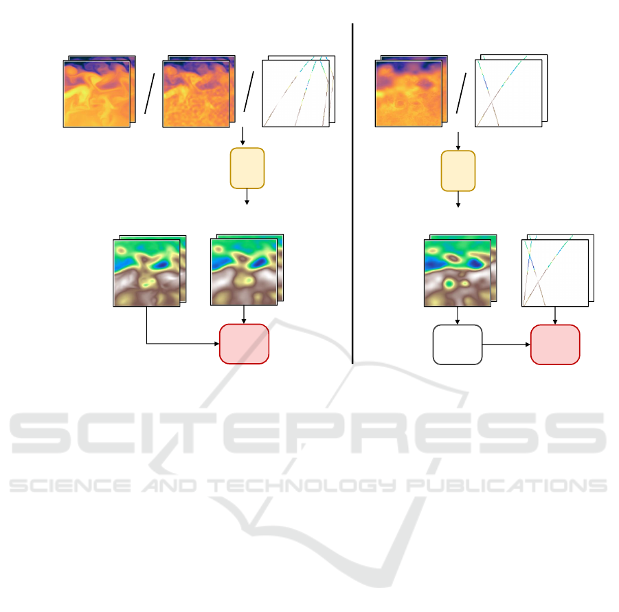
Figure 3: Computational graph of the two different training methods. In the supervised simulation situation (left) the neural

network f

takes as inputs either Y

ssh

alone, Y

ssh

and Y

sst

, or Y

ssh

and X

sst

. The network is then controlled in a supervised

manner. In the real-world observations framework (right), only a portion of satellite measures is passed to the network inputs

ssh

) with the SST optionally. The observing operator H

ssh

is then applied to the estimation

ssh

so that the network can be

controlled at the location where we have access to observations only.

3.3 Training Procedures

Using the two losses given in Section 3.2 and the two

datasets described in Section 2 several training and

ﬁne-tuning strategies are possible.

First, we can perform a supervised training on

the OSSE data, and directly infer real-world data.

This approach was tested by (Fablet et al., 2023) and

has the advantage of being straightforward, but could

suffer from the domain gap between the simulation

and the real world. Speciﬁcally, (Fablet et al., 2021)

achieved the training from SSH-only observations,

but, to this day, no SST-using method has successfully

been transferred to real-world data.

Another possibility is to train on real-world obser-

vations only using the loss described in Equation 3.

This approach was tested by (Archambault. et al.,

2023; Martin et al., 2023) which successfully in-

cluded SST information in SSH inpainting. How-

ever, comparing supervised and unsupervised meth-

ods on this OSSE, our previous work shows a signif-

icant drop in reconstruction performances for the un-

supervised interpolations (Archambault et al., 2023).

To beneﬁt from the supervised training on simu-

lated data without suffering from the domain gap, we

propose to pre-train ABED on the OSSE and to ﬁne-

tune it on real-world data. In the pre-training step,

we test three input settings: Y

ssh

for SST-agnostics

networks, (Y

ssh

, Y

sst

) for networks pre-trained with

SST observations, and (Y

ssh

, X

sst

) for networks pre-

trained using SST ground truth. Speciﬁcally, com-

paring methods pre-trained with X

sst

or Y

sst

will

help us to understand the impact of our OSSE. How-

ever, while training directly from observations or ﬁne-

tuning, only Y

sst

is available, therefore we reﬁt every

network using the same SST observations.

3.4 Training Details

Train, Validation, Test Split. The dataset is parti-

tioned as follows: we use the year 2017 for testing,

and we validate our methods on three periods: (1)

from July 14, 2002, to July 28, 2003, (2) from Jan-

uary 5, 2008, to January 18, 2009, and (3) from June

28, 2013, to July 13, 2014. The remaining data is

used for training, except for 15-day periods set aside

to prevent data leakage on the validation or the test

set. The partition is the same for the OSSE data and

the real-world data.

Normalization and Preprocessing. We center and

reduce the data of the neural network using the mean

VISAPP 2024 - 19th International Conference on Computer Vision Theory and Applications

104

Table 1: Scores of the 10-member ensemble of the ABED inpainting. We test the following learning methods: “Observations”

(trained only with real-world data), “Simulation” (trained only with simulated data), and “Both” (pre-trained on simulation

and ﬁne-tuned on real-world data). When the network is pre-trained using X

sst

it is still ﬁne-tuned with Y

sst

Learning method

Input data

ssh

+ Y

sst

ssh

+ X

sst

µ σ

Observation 6.52 1.95 111 6.13 1.84 104 — — —

Simulation 6.35 1.9 112 6.2 1.87 108 6.85 2.22 111

Both 6.27 1.85 110 5.77 1.64 102 5.77 1.6 103

and standard deviation of the training data. We grid

SSH along-track data to a series of images of size

21 × 128 × 128, and we set every pixel without in-

formation to 0. We subtract to the daily SST images

the seasonal mean of SST, i.e. the mean of SST maps

across all years in our training dataset, taken for this

day of the year.

Optimization. We use the ADAM opti-

mizer (Kingma and Ba, 2017), with a starting

learning rate of 5.10

−5

and a multiplicative decay of

0.99. While ﬁne-tuning, the initial learning rate is set

to 10

−5

and the decay to 0.9.

Ensemble. To address the sensitivity of neural net-

work optimization to weight initialization, we adopt

an ensemble strategy by training ten networks for

each conﬁguration. Referred to as the “Ensemble es-

timation”, this approach involves averaging the SSH

maps generated by the networks. The Ensemble esti-

mation usually produces better estimations than each

member separately (Hinton and Dean, 2015), and

speciﬁcally for SSH estimation (Archambault et al.,

2023; Archambault. et al., 2023; Filoche et al., 2022).

4 RESULTS

4.1 Comparison of the Different

Methods

In the following analysis, we compare ABED interpo-

lations based on two distinct criteria: the learning ap-

proach employed and the input data. The comparison

involves three learning methodologies: unsupervised

learning on observations only, training on simulated

data with a direct inference on real-world data, and

a hybrid approach involving pre-training on simula-

tion and ﬁne-tuning on observations. Simultaneously,

we evaluate three distinct sets of inputs: SSH-only,

SSH and noised SST, and SSH and SST ground truth

(a conﬁguration only possible while training on sim-

ulation). We evaluate all methods on the along-track

data from a satellite left aside from the inputs. To be

coherent with some of the interpolations of the ocean

data challenge (CLS/MEOM, 2021), the evaluation is

done on a smaller area than the one used for training

(from 34° to 42° North and -65° to -55° West). We

want to stress that the data used for the evaluation are

not used as inputs by any of these methods and present

an instrumental white noise with a standard deviation

from 2 to 3 cm. We still evaluate with this data keep-

ing in mind that the noise is leading to overestimating

the errors of the methods.

We consider Root Mean Squared Error (RMSE)

on the independent satellite data and compute µ,

its temporal mean, and σ

, its temporal standard

deviation. We also compute the spatial power density

spectrum (PSD) of the error and of the independent

data and retrieve λ

(in km), the wavelength where

the PSD of the error equals the PSD of the reference.

It can be seen as the smallest wavelength that is at

least half resolved by the interpolation method. For

further details about the implementation of λ

, we

refer the reader to (Le Guillou et al., 2020). Table 1

presents the scores of the different settings.

Is Our OSSE Realistic? Through this experiment,

we are able to assess the realism of our OSSE on SSH

and SST simulated observations. When examining

the SSH-only methods, we ﬁnd a substantial improve-

ment in the methods trained on simulation compared

to the ones trained on the observations alone. Fine-

tuning also leads to a reconstruction improvement

although smaller than the one brought by the pre-

training. We conclude that the SSH observations are

correctly simulated. However, the SST-aware meth-

ods trained on real-world data perform better than the

one trained on simulation and even more so for the

one trained using the SST ground truth. This under-

lines the fact that the SST noise is not perfectly sim-

ulated, even if it is still more realistic than the ground

truth SST. We also see that the two SST methods

achieve very similar performances after being ﬁne-

tuned, this shows that given an efﬁcient transfer learn-

ing strategy, we do not necessarily need to pre-train

the network in a realistic setting. This point will be

further discussed in Section 5.2.

Pre-Training and Fine-Tuning Attention Based Encoder Decoder Improves Sea Surface Height Multi-Variate Inpainting

105

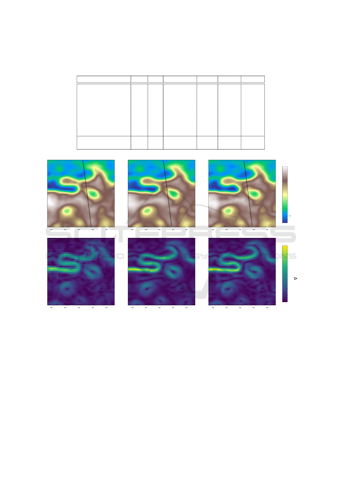
Table 2: Benchmark of the interpolations provided by (CLS/MEOM, 2021), including methods using SST or not, using neural

networks or not (NN), with different learning strategies. ABED interpolations are given for the pre-trained and ﬁne-tuned

version using SSH or SST.

Method SST NN Learning µ(cm) σ

(cm) λ

(km)

DUACS ✗ ✗ ✗ 7.66 2.66 138

DYMOST ✗ ✗ ✗ 6.75 2.00 121

MIOST ✗ ✗ ✗ 6.75 2.00 121

BFN ✗ ✗ ✗ 7.46 2.59 114

4DVarNet ✗ ✓ simulation 6.56 1.84 104

MUSTI ✓ ✓ observation 6.26 1.96 107

ConvLTSM-SSH ✗ ✓ observation 6.82 1.86 108

ConvLTSM-SSH-SST ✓ ✓ observation 6.29 1.60 102

ABED-SSH ✗ ✓ both 6.27 1.85 110

ABED-SSH-SST ✓ ✓ both 5.74 1.61 102

64 62 60 58 56

DUACS

64 62 60 58 56

ABED-SSH

64 62 60 58 56

ABED-SSH-SST

64 62 60 58 56

0.2

0.0

0.2

0.4

0.6

0.8

1.0

SSH(m)

0.0

0.2

0.4

0.6

0.8

1.0

1.2

1.4

1.6

SSH

1e 8

Figure 4: Estimated SSH maps from DUACS, ABED-SSH, ABED-SSH-SST and the norm of their spatial gradient. We plot the

trajectory of the satellite used for evaluation in Figure 5.

4.2 Comparison with State-of-the-Art

Data

We access the performance of our method by compar-

ing the ABED pre-trained and ﬁne-tuned inpaintings

to the state-of-the-art interpolations methods, on the

left-aside satellite data. The benchmarked methods

include DUACS, the most widely used product in oper-

ational applications (Taburet et al., 2019). We include

three physic-based data assimilation schemes: DY-

MOST (Ubelmann et al., 2016; Ballarotta et al., 2020),

MIOST (Ardhuin et al., 2020) and BFN (Le Guillou

et al., 2020). We also compare with the supervised

neural network 4DVarNet (Fablet et al., 2021), and

with neural networks trained using observations only

such as MUSTI (Archambault. et al., 2023) and the

ConvLTSM introduced by (Martin et al., 2023).

The results summarized in Table 2 show that

our method achieves state-of-the-art performances in

terms of RMSE among methods using only SSH and

methods using SST. More speciﬁcally, we see a clear

predominance of neural network-based methods as

well as SST-aware methods. ABED-SSH-SST thanks

to its pre-training and reﬁtting improves the recon-

struction of DUACS by 1.92 cm which acounts for

25% of its RMSE.

VISAPP 2024 - 19th International Conference on Computer Vision Theory and Applications

106

An Example of Improvement Brought by the SST.

Because of the absence of fully gridded ground truth

data in the real-world setup, the interpretation of the

results is difﬁcult. Nonetheless in Figure 4 we present

the estimated maps of the DUACS operational product,

as well as the one of ABED-SSH and ABED-SSH-SST.

We also compute the norm of the spatial gradient of

the SSH to highlight the areas of strong variations. Vi-

sually, we see smaller and more precise eddies in the

ABED inpainting, especially in the SST-aware version.

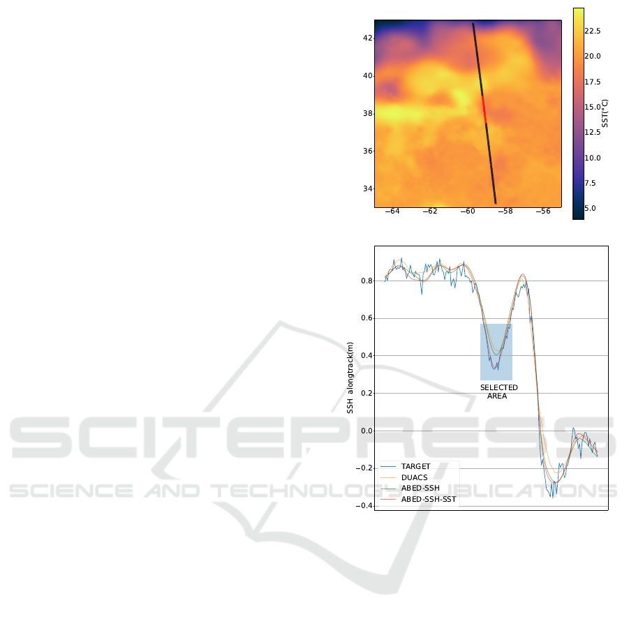
However, as it is still hard to show the impact of SST

on the reconstruction, we plot in Figure 5 the inter-

polation of the three different maps with the targeted

independent data. We select an area where an im-

provement is brought by the SST, as the SST-agnostic

methods clearly overestimate the SSH. When we plot

the trajectory of the satellite on the SST image we see

that the selected area corresponds to a small drop of

temperature. This is a typical example of the inter-

est in using temperature to constrain the inpainting as

this high-resolution information lacking in input SSH

observations.

5 CONCLUSIONS AND

PERSPECTIVES

5.1 Summary

Throughout this study, we successfully applied a

transfer learning strategy to perform the interpolation

of SSH using SST with an Attention-Based Encoder

Decoder. As in an operational scenario no fully grid-

ded ground truth is accessible to train the neural net-

work, we developed an Observing System Simulation

Experiment, a twin experiment that simulates the ob-

servation system of the satellites. Doing so, we were

able to compute pairs of realistic input/output based

on a physical simulation of the ocean and pre-train

our neural network. Then using an unsupervised loss

function we ﬁne-tuned the neural network on real-

world data. We show that the pre-training enhances

the reconstruction as our method achieves better re-

sults than the same network trained directly from ob-

servations. This is also the case for the ﬁne-tuned

version which outperforms the model solely trained

on simulated data proving the efﬁciency of the reﬁt-

ting. Benchmarking ABED with standard interpola-

tion methods, either based on physical prior models,

neural networks trained on simulations, or directly

from observations, we show that our training strategy

achieves state-of-the-art performances among SST-

aware or SSH-only methods. Compared to DUACS,

the most widely used oceanography product, we re-

Figure 5: An example of reconstruction improvement

brought by the SST. The SST image is represented along

with the trajectory of the evaluation satellite, as well as the

along-track interpolations of the three estimations presented

in Figure 4.

port an RMSE improvement of 1.92 cm out of the

7.66 cm of error (25% of the RMSE of DUACS) on

noised independent along-track data. We conclude

from this experiment that pre-train and ﬁne-tune neu-

ral networks help the reconstruction of variables, in

settings where no ground truth is available to con-

strain the inversion.

5.2 Discussions and Perspectives

Extension of the Methodology to Other Variables.

The proposed method could be applied to other input

or target variables if the following conditions are ful-

ﬁlled. First, the variables must be correlated to each

other, and we must have access to a realistic phys-

ical model that we can use to build a multi-variate

OSSE. The data generated through this mean can then

Pre-Training and Fine-Tuning Attention Based Encoder Decoder Improves Sea Surface Height Multi-Variate Inpainting

107

be used in the pre-training, enabling the network to

accurately learn the physical underlying link. Then

the ﬁne-tuning will adapt this learning to the noise of

the real-world data. One of the most obvious candi-

dates to serve as well as a target or input variable is

the sea’s Chlorophyll, which is a passive tracer of the

oceanic currents (Chelton et al., 2011).

Realism of the OSSE. We show that the multivariate

OSSE performed in this study was realistic, as well

for the SSH noise than for the SST noise. However,

given an appropriate transfer strategy, the networks

trained on the noised version of the SST and networks

trained on the ground truth SST achieve similar re-

sults once retrained. This leads us to reconsider the

necessity of computing a very realistic noise on con-

textual information, as the ﬁne-tuning process will get

rid of the learned features that do not appear in real-

world data.

Toward a Global Gridded Image. The experiment

that we performed in this work was focusing on a sin-

gle geographic area. Training a method able to es-

timate SSH on a global scale would require further

work. For instance, as the physical relationship be-

tween SSH and SST depends on latitude, we are cu-

rious to know if a global model would be competitive

compared to several local models.

REFERENCES

Amores, A., Jord

a, G., Arsouze, T., and Le Sommer, J.

(2018). Up to what extent can we characterize ocean

eddies using present-day gridded altimetric products?

Journal of Geophysical Research: Oceans, 123:7220–

7236.

Archambault., T., Filoche., A., Charantonis., A., and

eziat., D. (2023). Multimodal unsupervised spatio-

temporal interpolation of satellite ocean altimetry

maps. In Proceedings of the 18th International Joint

Conference on Computer Vision, Imaging and Com-

puter Graphics Theory and Applications (VISIGRAPP

2023) - Volume 4: VISAPP, pages 159–167. IN-

STICC, SciTePress.

Archambault, T., Filoche, A., Charantonis, A., B

eziat, D.,

and Thiria, S. (2023). Unsupervised learning of sea

surface height interpolation from multi-variate simu-

lated satellite observations. Submitted to Journal of

Advances of Modeling Earth Systems (JAMES).

Ardhuin, F., Ubelmann, C., Dibarboure, G., Gaultier, L.,

Ponte, A., Ballarotta, M., and Faug

ere, Y. (2020). Re-

constructing ocean surface current combining altime-

try and future spaceborne doppler data. Earth and

Space Science Open Archive.

Ballarotta, M., Ubelmann, C., Rog

e, M., Fournier, F.,

Faug

ere, Y., Dibarboure, G., Morrow, R., and Picot,

N. (2020). Dynamic mapping of along-track ocean al-

timetry: Performance from real observations. Journal

of Atmospheric and Oceanic Technology, 37:1593–

1601.

Bretherton, F., Davis, R., and Fandry, C. (1976). A tech-

nique for objective analysis and design of oceano-

graphic experiments applied to MODE-73. Deep-Sea

Research and Oceanographic Abstracts, 23:559–582.

Che, H., Niu, D., Zang, Z., Cao, Y., and Chen, X. (2022).

Ed-drap: Encoder–decoder deep residual attention

prediction network for radar echoes. IEEE Geoscience

and Remote Sensing Letters, 19.

Chelton, D. B., Gaube, P., Schlax, M. G., Early, J. J., and

Samelson, R. M. (2011). The inﬂuence of nonlinear

mesoscale eddies on near-surface oceanic chlorophyll.

Science, 334:328–332.

CLS/MEOM (2020). Swot data challenge natl60 [dataset].

CLS/MEOM (2021). Data challenge ose -

2021a ssh mapping ose [dataset].

CMEMS (2020). Global ocean physics reanalysis [dataset].

CMEMS (2021). Global ocean along-track l3 sea surface

heights reprocessed (1993-ongoing) tailored for data

assimilation [dataset].

Fablet, R., Amar, M., Febvre, Q., Beauchamp, M., and

Chapron, B. (2021). End-to-end physics-informed

representation learning for satellite ocean remote

sensing data: Applications to satellite altimetry and

sea surface currents. ISPRS Annals of the Photogram-

metry, Remote Sensing and Spatial Information Sci-

ences, 5:295–302.

Fablet, R., Febvre, Q., and Chapron, B. (2023). Multimodal

4dvarnets for the reconstruction of sea surface dynam-

ics from sst-ssh synergies. IEEE Transactions on Geo-

science and Remote Sensing, 61.

Filoche, A., Archambault, T., Charantonis, A., and

eziat, D. (2022). Statistics-free interpolation of

ocean observations with deep spatio-temporal prior.

In ECML/PKDD Workshop on Machine Learning for

Earth Observation and Prediction (MACLEAN).

Gaultier, L., Ubelmann, C., and Fu, L. (2016). The chal-

lenge of using future SWOT data for oceanic ﬁeld

reconstruction. Journal of Atmospheric and Oceanic

Technology, 33:119–126.

Guo, M.-H., Xu, T.-X., Liu, J.-J., Liu, Z.-N., Jiang, P.-T.,

Mu, T.-J., Zhang, S.-H., Martin, R. R., Cheng, M.-M.,

and Hu, S.-M. (2021). Attention mechanisms in com-

puter vision: A survey. Computational Visual Media,

8:331–368.

Hinton, G. and Dean, J. (2015). Distilling the knowledge in

a neural network. In NIPS Deep Learning and Repre-

sentation Learning Workshop.

Jam, J., Kendrick, C., Walker, K., Drouard, V., Hsu, J., and

Yap, M. (2021). A comprehensive review of past and

present image inpainting methods. Computer Vision

and Image Understanding, 203.

Kingma, D. P. and Ba, J. (2017). Adam: A method for

stochastic optimization.

Le Guillou, F., Metref, S., Cosme, E., Ubelmann, C., Bal-

larotta, M., Verron, J., and Le Sommer, J. (2020).

Mapping altimetry in the forthcoming SWOT era by

back-and-forth nudging a one-layer quasi-geostrophic

model. Earth and Space Science Open Archive.

VISAPP 2024 - 19th International Conference on Computer Vision Theory and Applications

108

Martin, S. (2014). An Introduction to Ocean Remote Sens-

ing. Cambridge University Press, 2 edition.

Martin, S. A., Manucharyan, G. E., and Klein, P. (2023).

Synthesizing sea surface temperature and satellite al-

timetry observations using deep learning improves the

accuracy and resolution of gridded sea surface height

anomalies. Journal of Advances in Modeling Earth

Systems, 15(5):e2022MS003589. e2022MS003589

2022MS003589.

McCann, M., Jin, K., and Unser, M. (2017). Convolutional

neural networks for inverse problems in imaging: A

review. IEEE Signal Processing Magazine, 34:85–95.

Nardelli, B., Cavaliere, D., Charles, E., and Ciani, D.

(2022). Super-resolving ocean dynamics from space

with computer vision algorithms. Remote Sensing,

14:1159.

NASA/JPL (2019). Ghrsst level 4 mur 0.25deg global

foundation sea surface temperature analysis (v4.2)

[dataset].

Qin, Z., Zeng, Q., Zong, Y., and Xu, F. (2021). Image in-

painting based on deep learning: A review. Displays,

69:102028.

Stegner, A., Le Vu, B., Dumas, F., Ghannami, M., Nicolle,

A., Durand, C., and Faugere, Y. (2021). Cyclone-

anticyclone asymmetry of eddy detection on gridded

altimetry product in the mediterranean sea. Journal of

Geophysical Research: Oceans, 126.

Taburet, G., Sanchez-Roman, A., Ballarotta, M., Pujol, M.-

I., Legeais, J.-F., Fournier, F., Faugere, Y., and Dibar-

boure, G. (2019). DUACS DT2018: 25 years of re-

processed sea level altimetry products. Ocean Sci,

15:1207–1224.

Thiria, S., Sorror, C., Archambault, T., Charantonis, A.,

eziat, D., Mejia, C., Molines, J.-M., and Crepon,

M. (2023). Downscaling of ocean ﬁelds by fusion of

heterogeneous observations using deep learning algo-

rithms. Ocean Modeling.

Ubelmann, C., Cornuelle, B., and Fu, L. (2016). Dynamic

mapping of along-track ocean altimetry: Method and

performance from observing system simulation exper-

iments. Journal of Atmospheric and Oceanic Technol-

ogy, 33:1691–1699.

Ulyanov, D., Vedaldi, A., and Lempitsky, V. (2017). Deep

image prior. International Journal of Computer Vi-

sion, 128:1867–1888.

Woo, S., Park, J., Lee, J.-Y., and Kweon, I. S. (2018). Cbam:

Convolutional block attention module. Computer Vi-

sion and Pattern Recognition.

Yang, J., Gong, P., Fu, R., Zhang, M., Chen, J., Liang, S.,

Xu, B., Shi, J., and Dickinson, R. (2013). The role

of satellite remote sensing in climate change studies.

Nature Climate Change 2013 3:10, 3:875–883.

Pre-Training and Fine-Tuning Attention Based Encoder Decoder Improves Sea Surface Height Multi-Variate Inpainting

109