An Analysis and Simulation Framework for Systems with Classiﬁcation

Components

Francesco Bedini

, Tino Jungebloud

, Ralph Maschotta

and Armin Zimmermann

Systems & Software Engineering Group, Technische Universit

at Ilmenau, Helmholtzplatz 5, Ilmenau, Germany

Keywords:

Ecore, EMF, SCPN, MMT, Classiﬁcation, Eclipse, Sirius, Xtext.

Abstract:

Machine learning solutions are becoming more widespread as they can solve some classes of problems better

than traditional software. Hence, industries look forward to integrating this new technology into their prod-

ucts and workﬂows. However, this calls for new models and analysis concepts in systems design that can

incorporate the properties and effects of machine learning components. In this paper, we propose a frame-

work that allows designing, analyzing, and simulating hardware-software systems that contain deep learning

classiﬁcation components. We focus on the modeling and predicting uncertainty aspects, which are typical

for machine-learning applications. They may lead to incorrect results that may negatively affect the entire

system’s dependability, reliability, and even safety. This issue is receiving increasing attention as “explain-

able” or “certiﬁable” AI. We propose a Domain-Speciﬁc Language with a precise stochastic colored Petri net

semantics to model such systems, which then can be simulated and analyzed to compute performance and re-

liability measures. The language is extensible and allows adding parameters to any of its elements, supporting

the deﬁnition of additional analysis methods for future modular extensions.

1 INTRODUCTION

Artiﬁcial intelligence (AI) and machine learning

(ML) are replacing conventional software in various

application ﬁelds (Shinde and Shah, 2018), thanks to

the increasing feasibility of deep learning (DL) ap-

proaches. The improvements in the training meth-

ods and the higher computing resources available on

demand and at more accessible prices make it possi-

ble to train a model with large training data to solve

classes of problems faster and better than traditional

software. Example of these problems includes image

recognition (Pak and Kim, 2017) and processing (Jiao

and Zhao, 2019), audio analysis (Schuller, 2013), and

speech recognition (Nassif et al., 2019). With the in-

creasing complexity and scale of these ML models

and the industrial applications they are about to be

used in, it becomes crucial to evaluate their perfor-

mance and assess their reliability.

A disadvantage of ML components from the sys-

tems and software engineering point of view is that

https://orcid.org/0000-0002-8354-1835

https://orcid.org/0000-0001-8319-9876

https://orcid.org/0000-0001-8447-3996

https://orcid.org/0000-0001-7439-7686

they behave in principle like black boxes without

a well-understood input-output function. They thus

may or may not deliver the correct result, depending

on multiple factors such as the quality, amount, diver-

sity, or cleansing (Maletic and Marcus, 2005) of the

training data (Liang et al., 2022) or seeing unexpected

data once in production.

ML suffers from two different kinds of uncertain-

ties: aleatoric (or statistical) uncertainty which is in-

herently related to a probabilistic choice itself that the

machine learning component performs and thus can-

not be eliminated, and the epistemic (or systematic)

uncertainty, which is caused by the lack of knowledge

of the model itself which can be reduced (Kiureghian

and Ditlevsen, 2009).

Using a closed-set classiﬁcation process as an ex-

ample, where the ML model has to assign its input

to a suitable class that describes it, even a perfectly

calibrated ML model with a very high detection rate

would generate wrong results whenever facing out-

of-distribution (OOD) inputs in production, despite

the high performance achieved on the known sample

distributions. The difﬁculty in detecting OOD cases

depends on how much the outliers are similar to the

known classes (Fort et al., 2021).

The quality of ML components can be evaluated

Bedini, F., Jungebloud, T., Maschotta, R. and Zimmermann, A.

An Analysis and Simulation Framework for Systems with Classiﬁcation Components.

DOI: 10.5220/0012357000003645

Paper published under CC license (CC BY-NC-ND 4.0)

In Proceedings of the 12th International Conference on Model-Based Software and Systems Engineering (MODELSWARD 2024), pages 50-61

ISBN: 978-989-758-682-8; ISSN: 2184-4348

thanks to different performance measures, each of

which should be carefully evaluated depending on the

use case (Flach, 2019). For classiﬁcation models, a

confusion matrix presents a tabular representation of

the model’s predictions against the actual class labels.

It provides insights into true positives (TPs), true neg-

atives (TNs), false positives (FPs), and false nega-

tives (FNs), allowing to calculate metrics like accu-

racy, precision, recall, and F1-score. These metrics

help understand the model’s performance for differ-

ent classes and identify areas of improvement.

1.1 Contribution

As black-box components are inherently hard to ver-

ify (Tappler et al., 2021) and industrial processes

rely on minimum qualitative standards that need to

be assured, the system-level effects of ML compo-

nents should be computable during the design phase.

One typical application is to decide about engineer-

ing trade-offs, such as between high accuracy and ef-

ﬁcient learning.

An integrated development environment (IDE)

shall allow the creation of system models using both a

graphical drag-and-drop interface and a textual nota-

tion, as the ﬁrst one is better suited for displaying re-

lationships between elements (Wile, 2004), whereas a

textual representation simpliﬁes inputting ﬁne details

and properties.

In order to provide a solid base for the analy-

sis methods that will be deﬁned in the framework, a

model-driven engineering (MDE) approach was fol-

lowed; the model semantics shall be easily under-

standable by the end-users but also have a precise se-

mantics to allow analyzing and simulating the model

instances in an unambiguous way. This was made

possible thanks to a transformation between the mod-

els and Stochastic colored Petri nets (SCPNs), which

describe the execution semantics of the domain-

speciﬁc language (DSL) with a token game.

With the proposed framework, we aim to provide

an easy-to-use model-based analysis and simulation

environment that supports domain experts in model-

ing and designing data ﬂows within systems’ com-

ponents. The contribution of this work is its holis-

tic approach that leads to a complete start-to-end sys-

tem analysis that considers the possible interactions

between different components instead of focusing on

the performance of single components.

This paper will focus on providing a high-level

overview of the entire analysis and simulation frame-

work for designing and validating systems that con-

tain components that may deliver uncertain outputs.

It describes the framework’s entire ﬂow and the main

conceptual points of the deﬁned DSL, focusing on the

preliminary results of the analysis of simple systems.

The remainder of this paper is structured as fol-

lows: Section 2 explores related works and pro-

vides background knowledge about modeling meth-

ods. Section 3 shows the framework’s big picture

and structure, whereas Section 4 shows the deﬁni-

tion of the DSL. Section 5 gives further details about

the analysis opportunities on the deﬁned models, and

Section 6 gives a short overview of the framework’s

technical realization. In conclusion, Section 7 shows

an application example, and Section 8 summarizes the

work and contains an outlook and ideas for future de-

velopments.

2 BACKGROUND

There are plenty of studies where AI gets applied

to software engineering methods (Zhang and Tsai,

2003), but only a few about applying a software en-

gineering methodology to analyze ML speciﬁcally at

the product or runtime application levels of the AI in

Software Engineering application levels (AI-SEAL)

taxonomy (Feldt et al., 2018), as in this work.

A different class of studies discusses applying an

engineering method to create machine learning mod-

els. For example, (Amershi et al., 2019) focuses on

the importance of applying a data-oriented engineer-

ing approach and deﬁnes a 9-step workﬂow after ana-

lyzing how software teams work with AI in Microsoft.

Traditional systems engineering approaches

worked well in the assumption that the processes

were almost deterministic (Pennock and Wade,

2015), whereas machine learning components are

probabilistic, meaning that they make predictions

based on statistical patterns observed in the training

data.

Publications related to the uncertainties caused by

ML, particularly about the importance and difﬁculty

of distinguishing aleatoric and epistemic uncertain-

ties, can be found in (H

ullermeier and Waegeman,

2021).

Regarding supervised ML, the labeled data avail-

able during training usually gets divided into three

sets: the training data, the validation data, and the test

data set (Suthaharan, 2016). Whereas the ﬁrst two

are actively used during the training process, the lat-

ter is the one used to compute performance measures

by evaluating the resulting model on fresh data it did

not see before.

How this data gets split between these three sets

may cause different classiﬁcation results and differ-

ent values of the performance measures. Cross-

An Analysis and Simulation Framework for Systems with Classiﬁcation Components

validation (Jiang et al., 2020) helps to assess the

model’s performance on unseen data and provides an

estimate of its generalization capability. A good bal-

ance between training and test sets is required (Xu and

Goodacre, 2018) to achieve a stable estimation of the

performance measures.

To the best of our knowledge, we are not aware

of comparable works about proposing a DSL able to

model a system containing ML-based classiﬁcation

components and analyze it in a holistic way. Graph-

ical editors that allow modeling ML elements such

as KNIME (O’Hagan and Kell, 2015) or AI dedi-

cated editors such as Artiﬁcial Intelligence Manage-

ment Software (AIMS) from AI-UI (AI-UI GmbH,

2022) do exist, but they also come with a ﬁxed seman-

tics which can not be changed. They are also more

focused on allowing users to actually use the machine

learning models rather than analyzing them.

Regarding the modeling possibilities available,

discrete-event models such as Petri nets (PNs) are

helpful for analyzing and simulating stochastic con-

current processes and systems, but lack readability by

systems designers and require speciﬁc knowledge to

use them. For this reason, a common approach con-

sists of using another kind of model that is simpler

to understand and whose semantics can be translated

automatically to a Petri net, such as in (Huang et al.,

2019), where Systems Modeling Language (SysML)

activity diagrams get veriﬁed after a transformation to

a PN.

These other models can either be known general-

purpose models such as Uniﬁed Modeling Language

(UML) or SysML, or a speciﬁc modeling language

designed for the speciﬁc purpose. For a language to

be fully speciﬁed, a deﬁnition of its semantics is re-

quired. We deﬁne our DSL’s precise semantics using

SCPNs directly, which is also the reason why General

Purpose Languages (GPLs) like UML or SysML has

not been used, in order to avoid confusion in its inter-

pretation in the case a different semantics needed to

be speciﬁed.

DSLs allow expressing domain knowledge con-

cretely, with direct involvement of the domain experts

with a modest implementation cost (Spinellis, 2001).

However, the literature shows that there is a gener-

alized lack of adoption of DSLs for various reasons,

for example related to social reluctance due to per-

ceived risks related to the DSL’s maintainability and

evolution (Tomassetti and Zaytsev, 2020) or such as

the lack of a simple formalized way to deﬁne a DSL

execution semantics (Bucchiarone et al., 2020).

Considering the implementation trade-offs listed

in (Mernik et al., 2005), and thanks to the improve-

ments in the ease of DSLs implementation due to

better tools, models, and languages than those avail-

able in 2005, realizing a DSL instead of expanding

generic modeling languages seems reasonable and is

supported by (Bonnet et al., 2016), where is acknowl-

edged that multi-purpose modeling languages such as

the UML for software and the SysML for systems are

not always the best option for implementing a model-

based systems engineering (MBSE) solution.

3 THE FRAMEWORK’S FLOW

This section provides a big-picture overview of the

operations that are supported by the framework and

how they are connected together.

User

Edit the

model

E4SM model

instance

Store the model

.e4sm

xml file

.e4smcode

MMT transformation

to SCPN

SCPN

Direct

analysis

Analysis

results

M2T transformation

HTML

documentation

Indirect

analysis

TimeNET

Figure 1: A data ﬂow diagram depicting the main ﬂows in-

side the framework. The yellow User and the simulation

software TimeNET are external entities. T depicts transient

data and D persistent data.

Our framework supports various operations, as

shown in Figure 1. The central object, which is used

by all activities, is the Engineering for Smart Manu-

facturing (E4SM) Model, an instance of our DSL.

The user can edit models (P1) either graphically

or textually as code. Models can then either be saved

as an XML ﬁle or as our speciﬁed code with the ex-

tension e4smcode (P2).

Both editors support a static model validation that

checks, for instance, that all cardinalities are met and

all deﬁned model constraints are respected (e.g., no

dangling edges are present in the model).

It is then possible to utilize the modeled system,

for example, by transforming it into other kinds of

models or documents. As a proof of concept, a gener-

ation of HTML-based model documentation through

a model-to-text (M2T) transformation has been im-

plemented (P3).

Once the system has been modeled, it is possible

to run two kinds of analysis, either direct ones straight

on the model instances (P4) or indirect ones against

a SCPN which gets generated by a model-to-model

transformation (MMT) (P5). In the second case, the

MODELSWARD 2024 - 12th International Conference on Model-Based Software and Systems Engineering

SCPN gets simulated thanks to an external software

called TimeNET (Zimmermann, 2008).

4 DSL DEFINITION

DSLs get written to provide a higher, more convenient

abstract conceptual level to users who are knowledge-

able in a particular area.

A fully speciﬁed DSL consists of an abstract

syntax (the metamodel), the semantics, and at least

one concrete syntax (how the language looks like to

users). To have a precise semantic, we are deﬁning

the semantics of our language with PN logic. In par-

ticular, we are using SCPNs (Zimmermann, 2012), to

support different kinds of tokens and give us the op-

portunity to have different channels for data and con-

trol ﬂows.

In order to allow the ﬁnal users to follow a top-

down or bottom-up design process, our DSL will al-

low specifying its elements hierarchically. Although

this will not eliminate any complexity, it will allow

making diagrams more comprehensible by hiding the

complexity of a single component in a further layer.

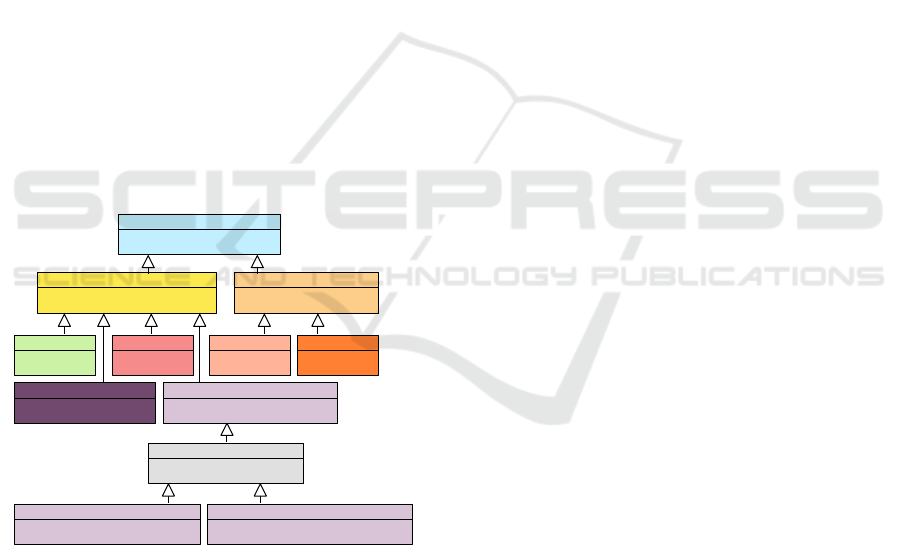
4.1 The Abstract Syntax

Component

Software Component

PhysicalComponent

Sensor

Actuator

Heuristic

Machine Learning Component

Function

External Dependency

Binary Classification Component

Multiclass Classification Component

Classification Component

Figure 2: A UML class diagram showing the components

hierarchy, without their attributes and operations. The color

palette used is the same that is used for the corresponding

model elements on the graphical editor.

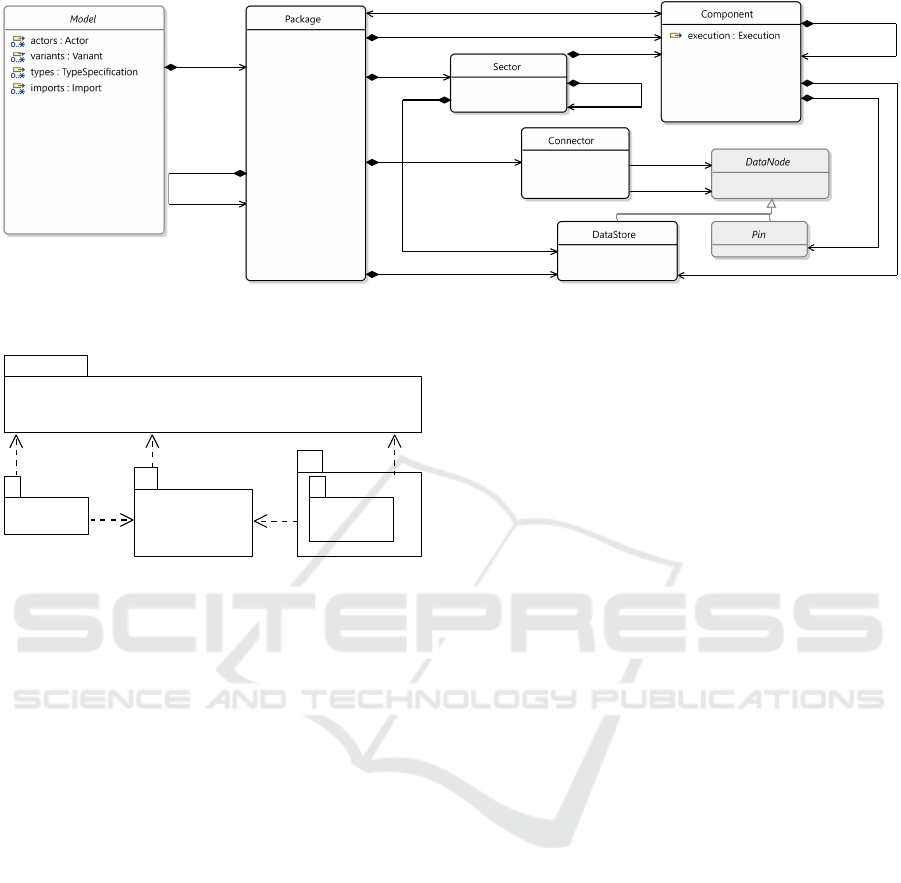
Due to space constraints, only the most important and

speciﬁc parts of the abstract syntax will be shown in

this work as Ecore class diagrams. In Figure 3, the

classes describing the most important structural ele-

ments are shown. A Model is the root element of our

DSL and holds all global elements, such as the ac-

tors, the variants, type speciﬁcation, and other model

imports. Models contain Packages, which are equiv-

alent to folders containing elements that are related to

each other. Packages can be contained recursively by

other packages. Though it is not a compulsory choice,

a package usually corresponds to a diagram. Inside

packages, Sectors can be used to group components

that belong together, either for their physical location

or just conceptually. Sectors do not add any seman-

tical meaning and have no inﬂuence on the system’s

execution.

The more used and central element type is the

Component. There are nine different types of compo-

nents, divided into two categories, software and phys-

ical components, as shown on the class diagram on

Figure 2. Components can contain other components,

or can be deﬁned hierarchically by another package,

in order to allow less cluttered high-level views sup-

porting a top-down approach.

Software components may, of course, not contain

physical components. Such restrictions are deﬁned by

constraints, which will be checked during model val-

idation and are also enforced by the graphical model

editor.

A generic placeholder component type is also

available to allow designing a system without need-

ing to know how each element will be realized in the

ﬁnal design.

As the DSL can also be used to distribute and

manage the work of different people, it is possible

to assign a Person (subclass of Actor) as main-

Responsible of a given component.

Components can have input and output pins,

which get connected by directed Connectors, which

can also be speciﬁed further as logical connectors or

physical connectors. Different kinds of components

allow for storing different information in the model.

For example, software components allow specify-

ing a degree of concurrency (number of servers) and

whether the execution is synchronous or not. The

same applies to connectors.

Physical connectors represent physical cables,

tracks on printed circuit boards, or wireless connec-

tions between physical components, whereas logi-

cal connectors represent data ﬂows exchanged within

physical components as packages. Similar to the

generic components, generic connectors are also

available and can be used as temporary placeholders

while designing a system at its early stages.

DataNodes are elements that can store data pack-

ages. Pins deﬁne the interface of components,

whereas DataStores can hold data indeﬁnitely once

they receive it. When newer data is provided, it re-

places the former value.

Figure 4 shows the metamodel’s package structure

and the dependencies between them. Five packages

An Analysis and Simulation Framework for Systems with Classiﬁcation Components

[0..*] sectors

[0..*] components

[0..*] packages

[0..*] components

[0..*] sectors

[0..*] packages

[0..1] specifiesComponent

[0..1] specifiedInPackage

[0..*] datastores

[0..*] connectors

[1..1] source

[1..1] target

[0..*] pins

Figure 3: An Eclipse Modeling Framework core meta model (Ecore) class diagram showing a small extract of the abstract

syntax.

E4SM

Core

Execution

Analysis

Results

Figure 4: A UML package diagram showing the package

hierarchy and dependencies.

have been deﬁned, which can be described as follows:

Core: this core package contains the fundamental el-

ements which are required by most of the other

packages, such as the data types and basic ele-

ments such as Element and NamedElement;

E4SM: this package is the main package and con-

tains, for example, the speciﬁcation of the com-

ponents, sectors, and pins;

Execution: this package contains all elements re-

lated to the speciﬁcation of the components’ ex-

ecution. It allows components to change the rate

of items ﬂowing between input and output pins,

and to change their data type;

Analysis: this package is used to specify elements

that are related to the analysis functions, such as

the deﬁnition of Parameters, which can be at-

tached to most of the model’s elements;

Results: subpackage of Analysis, is used to deﬁne

how the analysis results are structured and thus

deﬁnes the output interface of the analysis tools.

In this way, analysis results can be stored as mod-

els and be analyzed or displayed in a structured

way.

For each package, its namespace corresponds to

a lowercase version of its name. Namespaces are

required for having a unique name resolution in the

Eclipse Modeling Framework (EMF) and various

Eclipse plugins.

4.1.1 Classiﬁcation Components

For the simulation process to correctly reﬂect the

behavior of the classiﬁcation components, the com-

ponents’ performance measures (Diego et al., 2022)

such as accuracy, speciﬁcity, and recall are required.

It would be rather easy for the ﬁnal users to pro-

vide single values such as the accuracy for a given

class i (Equation (1)), which describes how many cor-

rect results (i.e., TPs and TNs) were delivered out of

all inputs. Other measures of observational error re-

quired by the simulation are the recall (Equation (2))

and the speciﬁcity (Equation (3)). The recall describes

the ratio between how many times a given class was

detected correctly out of all samples that should have

been detected as positive (i.e., the TPs summed with

the FNs), whereas the speciﬁcity, on the other hand,

shows how well the classiﬁcation component could

correctly classify a negative sample.

For the multiclass classiﬁcation case, aggregated

measures are available (Grandini et al., 2020), such as

balanced accuracy (Equation (4)), weighted balanced

accuracy (Equation (5)), micro average recall (Equa-

tion (6)), and macro average recall (Equation (7)).

Each of them has different strengths and shall be used

in different cases, depending, for example, on how

balanced the different classes are.

As all of these and other metrics can be easily

computed once the confusion matrix of a classiﬁca-

tion component is available, the DSL supports the de-

scription of binary and multiclass confusion matrices

in order not to restrict which kind of measure can be

used in the analysis phases. The metamodel provides

operations that can compute the most used measures

out of the box.

MODELSWARD 2024 - 12th International Conference on Model-Based Software and Systems Engineering

For a given class i:

accuracy

T P

+ T N

T P

+ FP

+ T N

+ FN

(1)

recall

T P

+ FN

(2)

speci f icity

T N

+ FP

(3)

For I classes, where w

describes the frequency of

the class i and W is the sum of all weights:

balAccuracy =

∑

i=0

recall

(4)

weiBalAccuracy =

∑

i=1

T P

(T P

+FN

)·w

I ·W

(5)

microRecall =

∑

i=0

T P

∑

i=0

(T P

+ FN

)

(6)

macroRecall =

∑

i=0

recall

(7)

Figure 5 shows the abstract syntax of the binary

classiﬁcation components, with a selection of the

most important attributes and operations.

We support two kinds of confusion matrices

(Binary- and Multiclass-ConfusionMatrix) and

the two respective types of classiﬁcation components,

which can hold multiple confusion matrices of the

appropriate type. Though classiﬁcation components

only have one confusion matrix in reality, multiple

matrices are supported in order to allow comparing

different variants during the simulation.

Inside Models, it is possible to specify

Environments which deﬁne how likely it is for the

systems’ sensors to detect a given Classification-

Class. This will be useful during the simulation to

test the component against situations where classes

have a different balance. Sensors can deﬁne what

classes they detect, and the confusion matrices deﬁne

what classes are detectable by the classiﬁcation

components.

4.2 The Concrete Syntax

Two concrete syntaxes have been deﬁned for this

DSL, a graphical concrete syntax and a textual con-

crete syntax.

4.2.1 The Graphical Concrete Syntax

The graphical concrete syntax is particularly useful

when modeling the system structure, the containment

relations of the components, and the connections be-

tween them. In order to lower the barrier for do-

main experts who would need to learn a completely

new concrete syntax, it is preferred to adopt existing

notations as much as possible (Karsai et al., 2014).

For this reason, our graphical notation is inspired by

UML’s component and activity diagrams.

Components are represented by rectangles, which

can contain squares on their edges denoting their in-

put (white, with an IN), output (gray, with an O), or

gateway (white or gray, with a G) pins. Gateway pins

connect a component to one of its internal compo-

nents, or vice-versa. Pins are connected by physi-

cal connectors (black arrows) between physical com-

ponents, or logical connectors (white arrows) within

components. Each component type has a different

color, and the initial of the type or an icon (for clas-

siﬁcation components) is displayed together with the

component’s name.

Sectors are logical or physical sections for com-

ponents. They are drawn as gray rectangles around

a set of components. Components can also act like

containers, as soon as they contain other components

which specify their internal structure or behavior.

Figure 6 shows a valid diagram depicting a pos-

sible modeling of a smart trafﬁc light with ML-based

vehicle classiﬁcation.

4.2.2 The Textual Concrete Syntax

model Example {

package Main {

p h ysi c a l C o nne c t o r con ” S1 . s en . s e n o u t ”

−> ” S1 . a c t . a c t i n ”

s e c t o r S1 {

components {

s e n s o r s e n {

doc : ”A d e s c r i p t i o n ”

t a k e s Det ( 3 3 )

ou t MyType s e n o u t

} ,

a c t u a t o r a c t {

i n MyType a c t i n

}

} } } }

Listing 1: An e4smcode example.

As the graphical concrete syntax would get too

cluttered to display model elements and attributes

graphically, the textual concrete syntax allows

expressing details (for example, about the internal

execution of the components) in a more concise and

An Analysis and Simulation Framework for Systems with Classiﬁcation Components

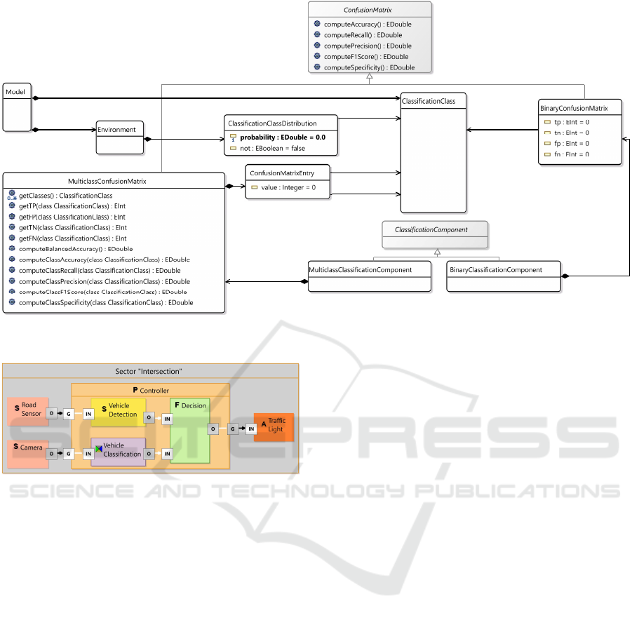
[0..*] confusionMatrixes

[0..*] entries

[0..*] environments

[0..*] classificationClasses

[1..1] predicted

[1..1] truth

[1..1] positiveClass

[0..*] classificationClasses

[1..1] classificationClass

Figure 5: An Ecore diagram showing the abstract syntax related to the different kinds of classiﬁcation components, confusion

matrices and the environment deﬁnition.

Figure 6: An example of a valid diagram with components

of different types contained in one sector. Black arrows de-

pict physical connectors, and white arrows represent logical

connectors.

practical way. The syntax is JSON-like and consists

in blocks that deﬁne elements, with the following

structure:

<elementType> <name > {< attribut e s and

chi ldre n >}

Whereas connectors are described with:

<connectorType> <name > " s o u rce " -> "

targ e t " where “source” and “target” are names-

paced and scoped strings leading to a model element

by its name, which corresponds to its ID. Double

quotes must surround names containing spaces.

Listing 1 shows a simple example of a sensor in-

side a sector directly connected to an actuator by a

physical connector. Here, it is possible to specify de-

tails that are not directly visible on the diagrams, such

as element descriptions, pin data types, or how often

a sensor executes.

4.3 The Semantics

Our DSL has a well-deﬁned execution semantics, as

deﬁned in (Mernik et al., 2005), speciﬁed solely by a

SCPN transformation. For this reason, our DSL can

also be seen as a high-level SCPN.

Showing the entire SCPN bijection speciﬁcation

formally for each structural metamodel element will

be out of scope for this paper and will be explained

in detail in an upcoming dedicated publication. Here,

only an informal description of the semantics is pro-

vided.

Components receive input and generate output to-

kens through their interface, which is deﬁned by their

pins. By default, each input pin awaits for an input

token, and each output pin generates an output token.

Optionally, input pins can collect multiple tokens, and

output pins can generate more than an output token.

A component starts its execution when each input pin

receives the set amount of tokens, but it is possible

to specify an or execution logic when a component

execution starts as soon as one input receives data.

As it is possible to connect multiple connectors to

one pin, each pin is allowed to specify what should

happen to the data when it is connected to multiple

connectors.

FCFS: First come, ﬁrst served; when multiple output

connectors from a pin are available, only one will

receive the data.

Duplicate: the data token gets duplicated and sent to

all the outgoing connectors concurrently.

MODELSWARD 2024 - 12th International Conference on Model-Based Software and Systems Engineering

Merge: when multiple input connectors reach a pin,

the data are collected together and merged into a

single data token.

Merge and Duplicate: when a pin has both multiple

input and outgoing connectors (e.g., in Gateway

pins), both merge and duplicate can be enabled.

Sensors, Actuators, and Classiﬁcation compo-

nents behave differently than all others. Sensors can

specify what kind of data they generate and with

which frequency, using different time distribution

functions. Actuators can only have input pins, and

they consume the tokens they receive, taking them out

of the system. Classiﬁcation components, thanks to

the information available through the confusion ma-

trix, behave as gray boxes. The way they get to exe-

cute is the same as all other components, but they ad-

ditionally classify the received class to one of its four

possible outcomes (TP, TN, FP, FN) based on metrics

derived from the confusion matrix.

5 ANALYSIS OPTIONS

After the model has been deﬁned, it is possible to

perform two kinds of analysis. Either directly on

the EMF model instances (Section 6.1) or by ana-

lyzing/simulating the SCPN resulting from the MMT

(Section 6.2).

With the component deﬁned in the Analysis and

Analysis Results packages, it is possible to deﬁne

analysis tools to compute any parameter of interest. In

this project, we aim to compute the following prop-

erties by running direct analyses on the EMF model

instance:

Execution Time: of particular interest in the case of

real-time systems with hard deadlines.

Network Usage: in order to assure that the planned

physical connections between components have

the necessary capacity to support their maximum

trafﬁc.

Errors Propagation: due to the uncertainties which

are intrinsic to the ML components or heuristics,

a simulation about their propagation in the system

is necessary.

Thanks to the classes Parameter and

ParameterDefinition, it is possible to deﬁne

and assign a parameter to almost any model element

to arbitrarily extend the attributes that can be stored

in our model. These can then be deﬁned and queried

by the analysis framework to support new kinds of

analysis.

6 IMPLEMENTATION

Our DSL has been implemented using Eclipse Mod-

eling Tools IDE, extended with Eclipse Sirius (Obeo,

2022b). A viable alternative would have been the

Meta Programming System (MPS) from JetBrains,

but Eclipse currently has more customizable graphical

editors and has a better holistic approach to support all

required model editors, MMT and M2Ts transforma-

tions.

The metamodel has been realized with the EMF

as a set of ecore ﬁles (one per package). The

EMF (Steinberg et al., 2008) is a well-known open-

source toolkit for developing DSLs (Gronback, 2009)

and allows to easily generate a default customizable

tree editor, which stores, by default, model instances

in an XML format. In order to support a more

comprehensible textual syntax, we used Xtext (The

Eclipse Foundation, 2022b; Bettini, 2016). Xtext au-

tomatically generates from a deﬁnition ﬁle an ANTLr

grammar (Parr and Quong, 1995), a textual editor

with plenty of useful features, such as auto-complete

with model elements scoping, syntax checking, and

model validation with visual feedback directly on the

code.

Regarding the graphical editor, we have deﬁned a

Sirius viewpoint speciﬁcation project, which allows

the ﬁnal users to create different kinds of representa-

tion:

Data Transfer Diagrams (DTD): are the main dia-

gram of this DSL and allow displaying the ﬂow

of data between components. Different layers are

available to allow different editing modes, such

as: Generic Elements to highlight elements that

have not been fully speciﬁed yet; Responsibilities

to highlight elements that do not have a main re-

sponsible or show the responsible person of com-

ponents who have it; Slow ﬂows to colorize the

connectors in a different shade depending on their

capacity; Missing Types highlights pin without a

speciﬁed type.

Component Speciﬁcation Diagrams (CSD): is

a diagram that allows specifying the internal

execution of a component within its input and

output pins.

Class Diagrams (CD): inspired from the UML class

diagram, it allows deﬁning domain-speciﬁc data

types and their relationships (inheritance and con-

tainment).

Person Management Table (PMT): is a table that

allows to easily edit all persons available in the

model and see all their responsibilities.

An Analysis and Simulation Framework for Systems with Classiﬁcation Components

Documentation Table (DOCT): is a table that al-

lows documenting the elements of the model. El-

ements that are missing a documentation text get

highlighted in this view.

Thanks to a M2T transformation realized with Ac-

celeo (Obeo, 2022a), it is possible to generate a web-

site listing all documentation annotations available in

the model, where all related elements are linked.

6.1 Direct Analyses

Direct analysis methods can be speciﬁed program-

matically as Java applications that use the interfaces

provided by our analysis package and the generated

EMF model interface. Direct analyses must be pro-

grammed manually and have complete access over all

attributes and the structure deﬁned in the EMF model

instance.

Analyses methods can be easily started from

within the Eclipse application, directly from the di-

agram’s context menu.

Currently, the analysis framework has been imple-

mented at a proof of concept level. It is possible to run

a simple execution time analysis that computes a path

between components and the required execution time

between these as a base for a more advanced deadline

analysis, which can be relevant for real-time systems.

6.2 The Model to Model

Transformation

To show a simple example of the transformation, we

introduce a small model (Figure 7).

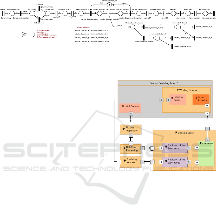
Figure 7: A simple model with a camera (input sensor),

a binary classiﬁcation component that can detect intruders,

and an alarm (actuator).

A camera with a ﬁxed framerate is connected to

a physical processing unit, which contains software

that can detect intruders on the frame through binary

classiﬁcation. The processing unit can send a signal

to an alarm system when needed.

Parsing the XML schema deﬁnition ﬁle (XSD),

which speciﬁes the structure of a valid SCPN, it was

possible to infer a metamodel that could be used as a

starting point to deﬁne a valid EMF model.

Using that metamodel as the target, a MMT has

been deﬁned in order to translate the model seman-

tic and execution logic to a valid, equivalent SCPN.

The transformation has been implemented with the

tool Eclipse QVT Operational (QVTo) (The Eclipse

Foundation, 2022a), which is fully integrated with the

Eclipse platform and can be started directly from the

Sirius editor.

The transformation automatically adds measures

for recording how many tokens are generated by sen-

sor nodes and how many tokens reach actuators to

support input/output analysis directly. When classi-

ﬁcation components are present, additional measures

for all their possible outcomes are also generated.

These will be used to compute the simulated perfor-

mance measures.

The simulation of the resulting SCPN aims to

evaluate how the classiﬁcation components behave

when the environment changes, for example, regard-

ing multiclass classiﬁers, allowing to provide a cer-

tain percentage of OOD samples which will always

be classiﬁed wrong, as the model was not trained on

it. Another option would be to try out a different dis-

tribution of classes to see if it would perform better or

worse if located in a different environment.

After the transformation, a small JavaScript appli-

cation that can be run locally with the cross-platform

runtime environment Node.js can be used to sim-

plify the resulting SCPN. This is done by removing

all superﬂuous immediate transitions (Recalde et al.,

2006), which just transfer tokens without modifying

them, as they would not contribute to the PN reach-

ability graph and can be removed without affecting

analysis or simulation results.

As the layout information cannot be easily trans-

ferred between the original EMF model and the

SCPN, as the output model has plenty elements more

than the original one and the size of the input ele-

ments varies vastly whereas the PN elements are ho-

mogeneous and small, the generated PN elements do

not contain any information regarding their graphical

distribution on the canvas. TimeNET comes with a

functionality that allows to automatically layout the

diagram elements using different Eclipse layout ker-

nel (ELK) algorithms. The ELK layered is the one

that usually works best for our kind of net.

Figure 8 shows the result of the automatic trans-

formation process of the model shown in Figure 7,

after the automatic simpliﬁcation and layout process

(manually adjusted for this publication). After the to-

ken gets initialized, it gets sent to the Intruder detec-

tion component. There, it will be picked through local

guards on the transitions if the sample belongs to the

Truth Class or not. If it belongs to the truth class,

the simulation will decide if it results in a TP or a FN

outcome, depending on the recall computed from the

MODELSWARD 2024 - 12th International Conference on Model-Based Software and Systems Engineering

cl_intruder (bool)

Figure 8: The simpliﬁed SCPN resulting from the MMT transformation of the model in Figure 7. 1 shows the data structure.

In 2, the data initialization is performed (in this case, it is set whether a class was detected or not). 3 shows the possibility of

limiting the execution of the components or simulating multi-core components via automatically generated semaphores. In

4, the performance-measures-based classiﬁcation results are drawn, and 5 shows the generated measures that will record the

four possible outcomes.

provided confusion matrix. On the other hand, if the

sample belongs to the other class, it can only come

out as a TN or a FP sample. This decision is taken

based on the model speciﬁcity.

The transformation has been validated through the

transformation of simple test cases, which led to the

expected results and their integration into progres-

sively larger models. A larger example of the transfor-

mation and simulation of a data stream pipeline can be

found in (R

ath et al., 2023). This work shows that a

pipeline can be modeled using our DSL, and the sim-

ulation of the automatically generated SCPN delivers

measures that match the real execution.

7 AN APPLICATION EXAMPLE

This section aims to provide an example of the kind

of models that can be realized using the framework,

considering that the resulting model needs to be small

enough to still be explainable and comprehensible

with the small graphics that can be placed on a scien-

tiﬁc paper, in particular with regards to the resulting

PN which naturally has a higher number of elements

than the original DSL model.

As an industrial example, we have used the sce-

nario described in the work of (Walther et al., 2022).

In that paper, a deep learning approach is used to pre-

dict the success of a laser beam butt welding process

of two sheets of high-alloy steel.

The diagram of the process, modeled using our

DSL, is shown in Figure 9. There are two sensors pro-

ducing data: an infrared camera supervising the weld-

ing process and an inductive probe sensor that mea-

sures how much the two sheets are diverging while

being welded. This data gets prepared and sent to two

different ML components, which will deliver their

prediction results to the controller. If a correction is

required, a signal is sent to the linear actuator, which

will push the two sheets back together with a certain

Figure 9: A diagram showing the high-level modeling of

the deep learning-controlled welding process.

strength.

This small model, composed of a total of 14 com-

ponents distributed in different packages, can be au-

tomatically transformed into a SCPN. The generated

SCPN contains 38 places and 38 transitions (30 timed

and 8 immediate) connected by 76 arcs. The simpliﬁ-

cation process allows obtaining an equivalent net that

contains 5 immediate transitions, 5 places, and 10 arcs

less.

The generated PN comes with measures for count-

ing the number of tokens generated by sensors and the

number of tokens consumed by actuators. This allows

performing an input/output response simulation based

on the given stochastic execution time and connection

capacity deﬁned in the model.

An Analysis and Simulation Framework for Systems with Classiﬁcation Components

8 CONCLUSION

In this work, we have shown the design and imple-

mentation of an open-source framework to deﬁne and

simulate data ﬂows within hardware-software sys-

tems containing ML components with uncertainties,

with an initial focus on binary classiﬁcation compo-

nents. The framework revolves around a DSL with

a precise SCPN semantics, which has been imple-

mented on the Eclipse environment (EMF) and in-

cludes an Eclipse Sirius graphical editor and an Xtext-

generated textual editor. The framework has been im-

plemented as a proof-of-concept and provides a start-

ing point for deﬁning different kinds of reusable sim-

ulations and analysis methods.

The presented approach makes it possible to con-

sider classiﬁcation components with known confu-

sion matrixes as gray boxes. The Petri net-based sim-

ulation process can mimic their behaviors based on

their performance measures computed from their test

data set.

The goodness of the simulation process regard-

ing the classiﬁcation components is correlated to the

amount and quality of the test data used to produce

the confusion matrices. If one class was poorly rep-

resented during the test phase, the computed perfor-

mance value may not correctly reﬂect reality.

8.1 Future Work

The upcoming steps include the implementation of

analysis methods for computing the network usage

and the deﬁnition of the simulation of the error prop-

agation inside the system. The implementation of a

simulation method for multi-label multiclass classiﬁ-

cation components is also planned, thanks to the work

of (Heydarian et al., 2022) towards the deﬁnition of

multi-label confusion matrices (MLCMs).

When the project leading to this work started in

2019, SysML v2 was still unavailable. Retrospec-

tively, it can be said that basing the DSL on Kernel

Modeling Language (KerML) (Jansen et al., 2022)

could provide a more ﬂexible base which more tools

in the future may support. When more mature tools

will be available, it may be worth considering rebas-

ing this DSL on KerML instead of Ecore to improve

its reusability and interoperability with more tools.

ACKNOWLEDGEMENTS

This work has received funding from the Carl Zeiss

Foundation as part of the project Engineering for

Smart Manufacturing (E4SM) under grant agreement

no. P2017-01-005.

REFERENCES

AI-UI GmbH (2022). Artiﬁcial intelligence user interface

(AI-UI). https://ai-ui.ai/en. last checked on Oct 2,

2024.

Amershi, S., Begel, A., Bird, C., DeLine, R., Gall, H., Ka-

mar, E., Nagappan, N., Nushi, B., and Zimmermann,

T. (2019). Software engineering for machine learn-

ing: A case study. In 2019 IEEE/ACM 41st Interna-

tional Conference on Software Engineering: Software

Engineering in Practice (ICSE-SEIP), pages 291–300,

New York, NY. IEEE.

Bettini, L. (2016). Implementing domain-speciﬁc languages

with Xtext and Xtend. Packt Publishing Ltd, Birming-

ham, United Kingdom.

Bonnet, S., Voirin, J.-L., Exertier, D., and Normand, V.

(2016). Not (strictly) relying on SysML for MBSE:

Language, tooling and development perspectives: The

Arcadia/Capella rationale. In 2016 Annual IEEE Sys-

tems Conference (SysCon), pages 1–6, Orlando, FL,

USA. IEEE.

Bucchiarone, A., Cabot, J., Paige, R. F., and Pierantonio, A.

(2020). Grand challenges in model-driven engineer-

ing: an analysis of the state of the research. Software

and Systems Modeling, 19(1):5–13.

Diego, I. M. D., Redondo, A. R., Fern

andez, R. R., Navarro,

J., and Moguerza, J. M. (2022). General perfor-

mance score for classiﬁcation problems. Applied In-

telligence, 52(10):12049–12063.

Feldt, R., de Oliveira Neto, F. G., and Torkar, R. (2018).

Ways of applying artiﬁcial intelligence in software en-

gineering.

Flach, P. (2019). Performance evaluation in machine learn-

ing: The good, the bad, the ugly, and the way forward.

Proceedings of the AAAI Conference on Artiﬁcial In-

telligence, 33(01):9808–9814.

Fort, S., Ren, J., and Lakshminarayanan, B. (2021). Ex-

ploring the limits of out-of-distribution detection. In

Ranzato, M., Beygelzimer, A., Dauphin, Y., Liang, P.,

and Vaughan, J. W., editors, Advances in Neural Infor-

mation Processing Systems, volume 34, pages 7068–

7081, Red Hook, NY, USA. Curran Associates, Inc.

Grandini, M., Bagli, E., and Visani, G. (2020). Metrics for

multi-class classiﬁcation: an overview.

Gronback, R. C. (2009). Eclipse modeling project: a

domain-speciﬁc language (DSL) toolkit. Pearson Ed-

ucation, London, United Kingdom.

Heydarian, M., Doyle, T. E., and Samavi, R. (2022).

Mlcm: Multi-label confusion matrix. IEEE Access,

10:19083–19095.

Huang, E., McGinnis, L. F., and Mitchell, S. W. (2019).

Verifying SysML activity diagrams using formal

transformation to Petri nets. Systems Engineering,

23(1):118–135.

MODELSWARD 2024 - 12th International Conference on Model-Based Software and Systems Engineering

ullermeier, E. and Waegeman, W. (2021). Aleatoric and

epistemic uncertainty in machine learning: an intro-

duction to concepts and methods. Machine Learning,

110(3):457–506.

Jansen, N., Pfeiffer, J., Rumpe, B., Schmalzing, D., and

Wortmann, A. (2022). The language of SysML v2

under the magnifying glass. The Journal of Object

Technology, 21(3):3:1.

Jiang, T., Gradus, J. L., and Rosellini, A. J. (2020). Su-

pervised machine learning: A brief primer. Behavior

Therapy, 51(5):675–687.

Jiao, L. and Zhao, J. (2019). A survey on the new generation

of deep learning in image processing. IEEE Access,

7:172231–172263.

Karsai, G., Krahn, H., Pinkernell, C., Rumpe, B., Schindler,

M., and V

olkel, S. (2014). Design guidelines for do-

main speciﬁc languages.

Kiureghian, A. D. and Ditlevsen, O. (2009). Aleatory

or epistemic? does it matter? Structural Safety,

31(2):105–112.

Liang, W., Tadesse, G. A., Ho, D., Fei-Fei, L., Zaharia, M.,

Zhang, C., and Zou, J. (2022). Advances, challenges

and opportunities in creating data for trustworthy ai.

Nature Machine Intelligence, 4(8):669–677.

Maletic, J. I. and Marcus, A. (2005). Data cleansing. Data

mining and knowledge discovery handbook, pages 21–

36.

Mernik, M., Heering, J., and Sloane, A. M. (2005). When

and how to develop domain-speciﬁc languages. ACM

Computing Surveys, 37(4):316–344.

Nassif, A. B., Shahin, I., Attili, I., Azzeh, M., and Shaalan,

K. (2019). Speech recognition using deep neural net-

works: A systematic review. IEEE Access, 7:19143–

19165.

Obeo (2022a). Acceleo. https://www.eclipse.org/acceleo.

last checked on Oct 2, 2024.

Obeo (2022b). Eclipse sirius. https://www.eclipse.org/

sirius. last checked on Oct 2, 2024.

O’Hagan, S. and Kell, D. B. (2015). Software review: the

KNIME workﬂow environment and its applications in

genetic programming and machine learning. Genetic

Programming and Evolvable Machines, 16(3):387–

391.

Pak, M. and Kim, S. (2017). A review of deep learning in

image recognition. In 2017 4th International Confer-

ence on Computer Applications and Information Pro-

cessing Technology (CAIPT), pages 1–3, Kuta Bali,

Indonesia. IEEE.

Parr, T. J. and Quong, R. W. (1995). ANTLR: A predicated-

LL (k) parser generator. Software: Practice and Ex-

perience, 25(7):789–810.

Pennock, M. J. and Wade, J. P. (2015). The top 10 illusions

of systems engineering: A research agenda. Procedia

Computer Science, 44:147–154. 2015 Conference on

Systems Engineering Research.

ath, T., Bedini, F., Sattler, K.-U., and Zimmermann, A.

(2023). Interactive performance exploration of stream

processing applications using colored petri nets. In

Proceedings of the 17th ACM International Confer-

ence on Distributed and Event-based Systems, pages

191–194.

Recalde, L., Mahulea, C., and Silva, M. (2006). Improv-

ing analysis and simulation of continuous Petri nets.

In 2006 IEEE International Conference on Automa-

tion Science and Engineering, pages 9–14, Shanghai,

China. IEEE.

Schuller, B. W. (2013). Intelligent Audio Analysis. Springer

Berlin Heidelberg, Heidelberg, Germany.

Shinde, P. P. and Shah, S. (2018). A review of ma-

chine learning and deep learning applications. In

2018 Fourth International Conference on Comput-

ing Communication Control and Automation (IC-

CUBEA), pages 1–6, Pune, India. IEEE.

Spinellis, D. (2001). Notable design patterns for domain-

speciﬁc languages. Journal of systems and software,

56(1):91–99.

Steinberg, D., Budinsky, F., Merks, E., and Paternostro, M.

(2008). EMF: eclipse modeling framework. Pearson

Education, London, Great Britain.

Suthaharan, S. (2016). Supervised Learning Algorithms,

pages 183–206. Springer US, Boston, MA.

Tappler, M., Mu

skardin, E., Aichernig, B. K., and Pill, I.

(2021). Active model learning of stochastic reactive

systems. In Software Engineering and Formal Meth-

ods, pages 481–500. Springer International Publish-

ing, Cham, Switzerland.

The Eclipse Foundation (2022a). Eclipse QVT opera-

tional. https://projects.eclipse.org/projects/modeling.

mmt.qvt-oml. last checked on Oct 2, 2024.

The Eclipse Foundation (2022b). Xtext. https://www.

eclipse.org/Xtext. last checked on Oct 2, 2024.

Tomassetti, F. and Zaytsev, V. (2020). Reﬂections on the

lack of adoption of domain speciﬁc languages. In

STAF Workshops, pages 85–94.

Walther, D., Schmidt, L., Schricker, K., Junger, C.,

Bergmann, J. P., Notni, G., and M

ader, P. (2022). Au-

tomatic detection and prediction of discontinuities in

laser beam butt welding utilizing deep learning. Jour-

nal of Advanced Joining Processes, 6:100119.

Wile, D. (2004). Lessons learned from real DSL ex-

periments. Science of Computer Programming,

51(3):265–290.

Xu, Y. and Goodacre, R. (2018). On splitting training

and validation set: A comparative study of cross-

validation, bootstrap and systematic sampling for es-

timating the generalization performance of supervised

learning. Journal of Analysis and Testing, 2(3):249–

262.

Zhang, D. and Tsai, J. (2003). Machine learning and

software engineering. Software Quality Journal,

11(2):87–119.

Zimmermann, A. (2008). Stochastic Discrete Event Sys-

tems. Springer Berlin, Heidelberg, Heidelberg, Ger-

many.

Zimmermann, A. (2012). Modeling and evaluation of

stochastic Petri nets with TimeNET 4.1. In 6th In-

ternational ICST Conference on Performance Evalua-

tion Methodologies and Tools, pages 54–63, Cargese,

France. IEEE.

An Analysis and Simulation Framework for Systems with Classiﬁcation Components