Are Semi-Dense Detector-Free Methods Good at Matching Local
Features?
Matthieu Vilain, R
´
emi Giraud, Hugo Germain and Guillaume Bourmaud
Univ. Bordeaux, CNRS, Bordeaux INP, IMS, UMR 5218, F-33400 Talence, France
Keywords:
Image Matching, Transformer, Pose Estimation.
Abstract:
Semi-dense detector-free approaches (SDF), such as LoFTR, are currently among the most popular image
matching methods. While SDF methods are trained to establish correspondences between two images, their
performances are almost exclusively evaluated using relative pose estimation metrics. Thus, the link between
their ability to establish correspondences and the quality of the resulting estimated pose has thus far received
little attention. This paper is a first attempt to study this link. We start with proposing a novel structured
attention-based image matching architecture (SAM). It allows us to show a counter-intuitive result on two
datasets (MegaDepth and HPatches): on the one hand SAM either outperforms or is on par with SDF methods
in terms of pose/homography estimation metrics, but on the other hand SDF approaches are significantly
better than SAM in terms of matching accuracy. We then propose to limit the computation of the matching
accuracy to textured regions, and show that in this case SAM often surpasses SDF methods. Our findings
highlight a strong correlation between the ability to establish accurate correspondences in textured regions and
the accuracy of the resulting estimated pose/homography. Our code will be made available.
1 INTRODUCTION
Image matching is the task of establishing correspon-
dences between two partially overlapping images. It
is considered to be a fundamental problem of 3D com-
puter vision, as establishing correspondences is a pre-
condition for several downstream tasks such as struc-
ture from motion (Heinly et al., 2015; Sch
¨
onberger
and Frahm, 2016), visual localisation (Sv
¨
arm et al.,
2017; Sattler et al., 2017; Taira et al., 2018) or si-
multaneous localization and mapping (Strasdat et al.,
2011; Sarlin et al., 2022). Despite the abundant work
dedicated to image matching over the last thirty years,
this topic remains an unsolved problem for challeng-
ing scenarios, such as when images are captured from
strongly differing viewpoints (Arnold et al., 2022)
(Jin et al., 2020), present occlusions (Sarlin et al.,
2022) or feature day-to-night changes (Zhang et al.,
2021).
An inherent part of the problem is the difficulty to
evaluate image matching methods. In practice, it is
often tackled with a proxy task such as relative or ab-
solute camera pose estimation, or 3D reconstruction.
In this context, image matching performances were
recently significantly improved with the advent of
attention layers (Vaswani et al., 2017). Cross-
attention layers are mainly responsible for this break-
through (Sarlin et al., 2020) as they enable the lo-
cal features of detected keypoints in both images to
communicate and adjust with respect to each other.
Prior siamese architectures (Yi et al., 2016; Ono et al.,
2018; Dusmanu et al., 2019), (Revaud et al., 2019),
(Germain et al., 2020; Germain et al., 2021) had so
far prevented this type of communication. Shortly af-
ter this breakthrough, a second significant milestone
was reached (Sun et al., 2021) by combining the usage
of attention layers (Sarlin et al., 2020) with the idea
of having a detector-free method (Rocco et al., 2018;
Rocco et al., 2020a; Rocco et al., 2020b; Li et al.,
2020), (Zhou et al., 2021; Truong et al., 2021). In
LoFTR (Sun et al., 2021), low-resolution dense cross-
attention layers are employed that allow semi-dense
low-resolution features of the two images to commu-
nicate and adjust to each other. Such a method is said
to be detector-free, as it matches semi-dense local fea-
tures instead of sparse sets of local features coming
from detected keypoint locations (Lowe, 1999).
Semi-dense Detector-Free (SDF) methods (Chen
et al., 2022; Giang et al., 2023; Wang et al., 2022;
Sun et al., 2021), (Mao et al., 2022; Tang et al., 2022),
such as LoFTR, are among the best performing image
matching approaches in terms of pose estimation met-
Vilain, M., Giraud, R., Germain, H. and Bourmaud, G.
Are Semi-Dense Detector-Free Methods Good at Matching Local Features?.
DOI: 10.5220/0012353600003660
Paper published under CC license (CC BY-NC-ND 4.0)
In Proceedings of the 19th International Joint Conference on Computer Vision, Imaging and Computer Graphics Theory and Applications (VISIGRAPP 2024) - Volume 4: VISAPP, pages
35-46
ISBN: 978-989-758-679-8; ISSN: 2184-4321
Proceedings Copyright © 2024 by SCITEPRESS – Science and Technology Publications, Lda.
35

LoFTR+QuadTree SAM (ours)
MA@2=60.6 MA
text
@2=84.0 errR=2.1' errT=5.4'
MA@2=62.8 MA
text
@2=64.0 errR=5.5' errT=22.4'
Figure 1: Given query locations within textured regions
of the source image (left), we show their predicted corre-
spondents in the target image (right) for: (Top row) SAM
(Proposed) - Structured Attention-based image Matching,
(Bottom row) LoFTR (Sun et al., 2021)+QuadTree (Tang
et al., 2022) - a semi-dense detector-free approach (line
colors indicate the distance in pixels with respect to the
ground truth correspondent). We report: (MA@2) - the
matching accuracy at 2 pixels computed on all the semi-
dense locations of the source image with available ground
truth correspondent (which includes both textured and uni-
form regions), (MA
text
@2) - the matching accuracy at 2
pixels computed on all the textured semi-dense locations of
the source image with available ground truth correspondent
(i.e., uniform regions are ignored), (errR and errT) - the rel-
ative pose error. SAM has a better pose estimation but a
lower matching accuracy (MA@2), which seems counter-
intuitive. However, if we consider only textured regions
(MA
text
@2), then SAM outperforms LoFTR+QuadTree.
rics. However, to the best of our knowledge, the link
between their ability to establish correspondences and
the quality of the resulting estimated pose has thus far
received little attention. This paper is a first attempt
to study this link.
Contributions. We start with proposing a novel
Structured Attention-based image Matching architec-
ture (SAM). We evaluate SAM and 6 SDF methods
on 3 datasets (MegaDepth - relative pose estimation
and matching, HPatches - homography estimation and
matching, ETH3D - matching).
We highlight a counter-intuitive result on two
datasets (MegaDepth and HPatches): on the one hand
SAM either outperforms or is on par with SDF meth-
ods in terms of pose/homography estimation metrics,
but on the other hand SDF approaches are signifi-
cantly better than SAM in terms of Matching Accu-
racy (MA). Here the MA is computed on all the semi-
dense locations (of the source image) with available
ground truth correspondent, which includes both tex-
tured and uniform regions.
We propose to limit the computation of the match-
ing accuracy to textured regions, and show that in this
case SAM often surpasses SDF methods. Our find-
ings highlight a strong correlation between the abil-
ity to establish accurate correspondences in textured
regions and the accuracy of the resulting estimated
pose/homography (see Figure 1).
Organization of the Paper. Sec. 2 discusses the
related work. The proposed SAM architecture is in-
troduced in Sec. 3 and the experiments in Sec. 4.
2 RELATED WORK
Since this paper focuses on the link between the abil-
ity of SDF methods to establish correspondences and
the quality of the resulting estimated pose, we only
present SDF methods in this literature review and re-
fer the reader to (Edstedt et al., 2023; Zhu and Liu,
2023; Ni et al., 2023) for a broader literature review.
To the best of our knowledge, LoFTR (Sun et al.,
2021) was the first method to perform attention-based
detector-free matching. A siamese CNN is first ap-
plied on the source/target image pair to extract fine
dense features of resolution 1/2 and coarse dense fea-
tures of resolution 1/8. The source and target coarse
features are fed into a dense attention-based module,
interleaving self-attention layers with cross-attention
layers as proposed in (Sarlin et al., 2020). To reduce
the computational complexity of these dense attention
layers, Linear Attention (Katharopoulos et al., 2020)
is used instead of vanilla softmax attention (Vaswani
et al., 2017). The resulting features are matched to
obtain coarse correspondences. Each coarse corre-
spondence is then refined by cropping 5×5 windows
into the fine features and applying another attention-
based module. Thus for each location of the semi-
dense (factor of 1/8) source grid, a correspondent is
predicted. In practice, a Mutual Nearest Neighbor
(MNN) step is applied at the end of the coarse match-
ing stage to remove outliers.
In (Tang et al., 2022), a QuadTree attention mod-
ule is proposed to reduce the computational com-
plexity of vanilla softmax attention from quadratic
to linear while keeping its power, as opposed to
Linear Attention (Katharopoulos et al., 2020) which
was shown to underperform on local feature match-
ing (Germain et al., 2022). The QuadTree attention
module is used as a replacement for Linear Atten-
tion module in LoFTR. An architecture called ASpan-
Former is introduced in (Chen et al., 2022) that em-
ploys the same refinement stage as LoFTR but a dif-
ferent coarse stage architecture. Instead of classical
cross-attention layers, the coarse stage uses global-
local cross-attention layers that have the ability to
focus on regions around current potential correspon-
VISAPP 2024 - 19th International Conference on Computer Vision Theory and Applications
36

Structured
Cross-
Attention
CNN
Source PE
CNN
Target PE
Latent space
Learned
latent vectors
Query 2D locations
Structured
Self-
Attention
Structured
Cross-
Attention
Corresp.
Maps
: Dot product
xS
Source
Image
Target
Image
Softmax
Attention Maps
Structured Attention
(a) SAM architecture (b) Structured Attention
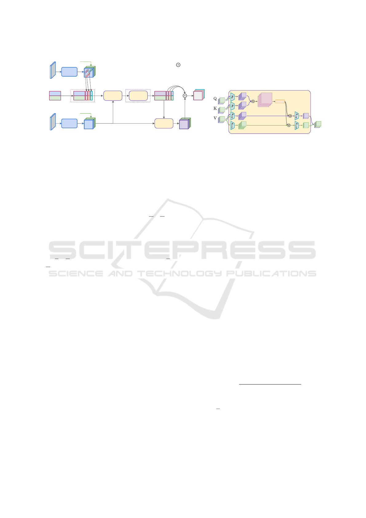
Figure 2: Overview of the proposed Structured Attention-based image Matching (SAM) method. (a) The matching
architecture first extracts features from both source and target images at resolution 1/4. Then it uses a set of learned latent
vectors alongside the descriptors of the query locations, and performs an input structured cross-attention with the dense
features of the target. The latent space is then processed through a succession of structured self-attention layers. An output
structured cross-attention is applied to update the target features with the information from the latent space. Finally, the
correspondence maps are obtained using a dot product. (b) Proposed structured attention layer. See text for details.
dences. MatchFormer (Wang et al., 2022) proposes an
attention-based backbone, interleaving self and cross-
attention layers, to progressively transform a tensor of
size 2×H ×W ×3 into a tensor of size 2×
H
16
×
W
16
×C.
Efficient attention layers such as Spatial Efficient At-
tention (Wang et al., 2021; Xie et al., 2021) and Lin-
ear Attention (Katharopoulos et al., 2020) are em-
ployed. A feature pyramid network-like decoder (Lin
et al., 2017) is used to output a fine tensor of size
2×
H
2
×
W
2
×C
f
and a coarse tensor of size 2×
H
8
×
W
8
×C
c
, and the matching is performed as in LoFTR.
TopicFM (Giang et al., 2023) follows the same global
architecture as LoFTR with a different coarse stage.
Here, topic distributions (latent semantic instances)
are inferred from coarse CNN features using cross-
attention layers with topic embeddings. These topic
distributions are used to augment the coarse CNN fea-
tures with self and cross-attention layers. In (Mao
et al., 2022), a method called 3DG-STFM proposes
to train the LoFTR architecture with a student-teacher
method. The teacher is first trained on RGB-D im-
age pairs. The teacher model then guides the student
model to learn RGB-induced depth information.
3 STRUCTURED
ATTENTION-BASED IMAGE
MATCHING ARCHITECTURE
In the following section, we present our novel Struc-
tured Attention-based image Matching architecture
(SAM), whose architecture is illustrated in Figure 2.
3.1 Background and Notations
Image Matching. Given a set of 2D query locations
{
p
s,i
}
i=1...L
in a source image I
s
, we seek to find their
2D correspondent locations
{
ˆ
p
t,i
}
i=1...L
in a target im-
age I
t
:
{
ˆ
p
t,i
}
i=1...L
= M

I
s
, I
t
,
{
p
s,i
}
i=1...L

. (1)
Here M is the image matching method. In the case of
semi-dense detector-free methods, the query locations
{
p
s,i
}
i=1...L
are defined as the source grid locations
using a stride of 8. As we will see, SAM is more
flexible and can process any set of query locations.
However, for a fair comparison, in the experiments
all the methods (including SAM) will use source grid
locations using a stride of 8 as query locations.
Vanilla Softmax Attention. A cross-attention op-
eration, with H heads, between a D-dimensional
query vector x and a set of D-dimensional vectors
{
y
n
}
n=1...N
can be written as follows:
H
∑
h=1
N
∑
n=1
1×1
z}|{
s
h,n
D×D
H
z}|{
W
o,h
D
H
×D
z}|{
W
v,h
D×1
z}|{
y
n
, (2)
where s
h,n
=
exp(
1×D
z}|{
x
⊤
D×D
H
z}|{
W
⊤
q,h
D
H
×D
z}|{
W
k,h
D×1
z}|{
y
⊤
n
)
∑
N
m=1
exp(x
⊤
W
⊤
q,h
W
k,h
y
m
)
. (3)
In practice, all the matrices W
·,·
are learned. Usu-
ally D
H
=
D
H
. The output is a linear combination (with
coefficients s
h,n
) of the linearly transformed set of
vectors
{
y
n
}
n=1...N
. This operation allows to extract
the relevant information in
{
y
n
}
n=1...N
from the point
of view of the query x. The query x is not an element
Are Semi-Dense Detector-Free Methods Good at Matching Local Features?
37

Source Image Target Image Average query map Average latent map
.
Figure 3: Visualization of the learned latent vectors of SAM. The average query map is obtained by averaging 64 correspon-
dence maps of 64 query locations (Red crosses) while the average latent map is obtained by averaging the 128 correspondence
maps of the 128 learned latent vectors. We observe that the average query map is mainly activated around the correspondents,
whereas these regions are less activated in the average latent map.
of that linear combination. As a consequence, a resid-
ual connection is often added, usually followed by a
layer normalization and a 2-layer MLP (with residual
connection) (Vaswani et al., 2017).
In practice, a cross-attention layer between a set
of query vectors
{
x
n
}
n=1...Q
and
{
y
n
}
n=1...N
is per-
formed in parallel, which is often computationally
demanding since, for each head, the coefficients are
stored in a Q×N matrix. A self-attention layer is a
cross-attention layer where
{
y
n
}
n=1...N
=
{
x
n
}
n=1...Q
.
3.2 Feature Extraction Stage
Our method takes as input a source image I
s
(H
s
×
W
s
× 3), a target image I
t
(H
t
×W
t
× 3) and a set of
2D query locations
{
p
s,i
}
i=1...L
. The first stage of
SAM is a classical feature extraction stage. From
the source image I
s
(H
s
×W
s
× 3) and the target im-
age I
t
(H
t
×W
t
× 3), dense visual source features F
s
(
H
s
4
×
W
s
4
× 128) and target features F
t
(
H
t
4
×
W
t
4
× 128)
are extracted using a siamese CNN backbone. The
Positional Encodings (PE) of the source and target are
computed, using an MLP (Sarlin et al., 2020), and
concatenated with the visual features of the source
and target to obtain two tensors H
s
(
H
s
4
×
W
s
4
×256) and
H
t
(
H
t
4
×
W
t
4
× 256). For each 2D query point p
s,i
, a
descriptor h
s,i
of size 256 is extracted from H
s
. In
practice, we use integer query locations thus there is
no need for interpolation here. Technical details con-
cerning this stage are provided in the appendix.
3.3 Latent Space Attention-Based Stage
In order to allow for the descriptors
{
h
s,i
}
i=1...L
(at
training-time we use L = 1024) to communicate and
adjust with respect to H
t
, we draw inspiration from
Perceiver (Jaegle et al., 2021; Jaegle et al., 2022),
and consider a set of N = M+L latent vectors, com-
posed of M learned latent vectors
{
m
i
}
i=1...M
and
the L descriptors
{
h
s,i
}
i=1...L
. These latent vectors

{
m
i
}
i=1...M
,
{
h
s,i
}
i=1...L

are used as queries in an
input cross-attention layer to extract the relevant in-
formation from H
t
, and finally obtain an updated set
of latent vectors
nn
m
(0)
i
o
i=1...M
,
n
h
(0)
s,i
o
i=1...L
o
. On
the one hand, the outputs
n
h
(0)
s,i
o
i=1...L
contain the
information relevant to find their respective corre-
spondents within H
t
. On the other hand, the outputs
n
m
(0)
i
o
i=1...M
extracted a general representation of H
t
since they are not aware of the query 2D locations.
In practice, we set M to 128. Afterward, a series of S
self-attention layers are applied to the latent vectors to
get
nn
m
(S)
i
o
i=1...M
,
n
h
(S)
s,i
o
i=1...L
o
. In these layers,
all latent vectors can communicate and adjust with re-
spect to each other. For instance, the set
n
m
(s)
i
o
i=1...M
can be used to disambiguate certain correspondences.
Then, H
t
is used as a query in an output cross-attention
layer to extract the relevant information from the la-
tent vectors. The resulting tensor is written H
out
t
. For
each updated descriptor h
(S)
s,i
, a correspondence map
C
t,i
(of size
H
t
4
×
W
t
4
) is obtained by computing the dot
product between h
(S)
s,i
and H
out
t
. Finally, for each 2D
query location p
s,i
, the predicted 2D correspondent
location
ˆ
p
t,i
is defined as the argmax of C
t,i
.
In Figure 3, we propose a visualization of the
learned latent vectors of SAM. For visualization pur-
poses, we used L = 64. Thus the average query map is
obtained by averaging the 64 correspondence maps of
the 64 query locations, while the average latent map is
obtained by averaging the 128 correspondence maps
of the 128 learned latent vectors. We observe that the
average query map is mainly activated around the cor-
respondents, whereas these regions are less activated
in the average latent map.
VISAPP 2024 - 19th International Conference on Computer Vision Theory and Applications
38

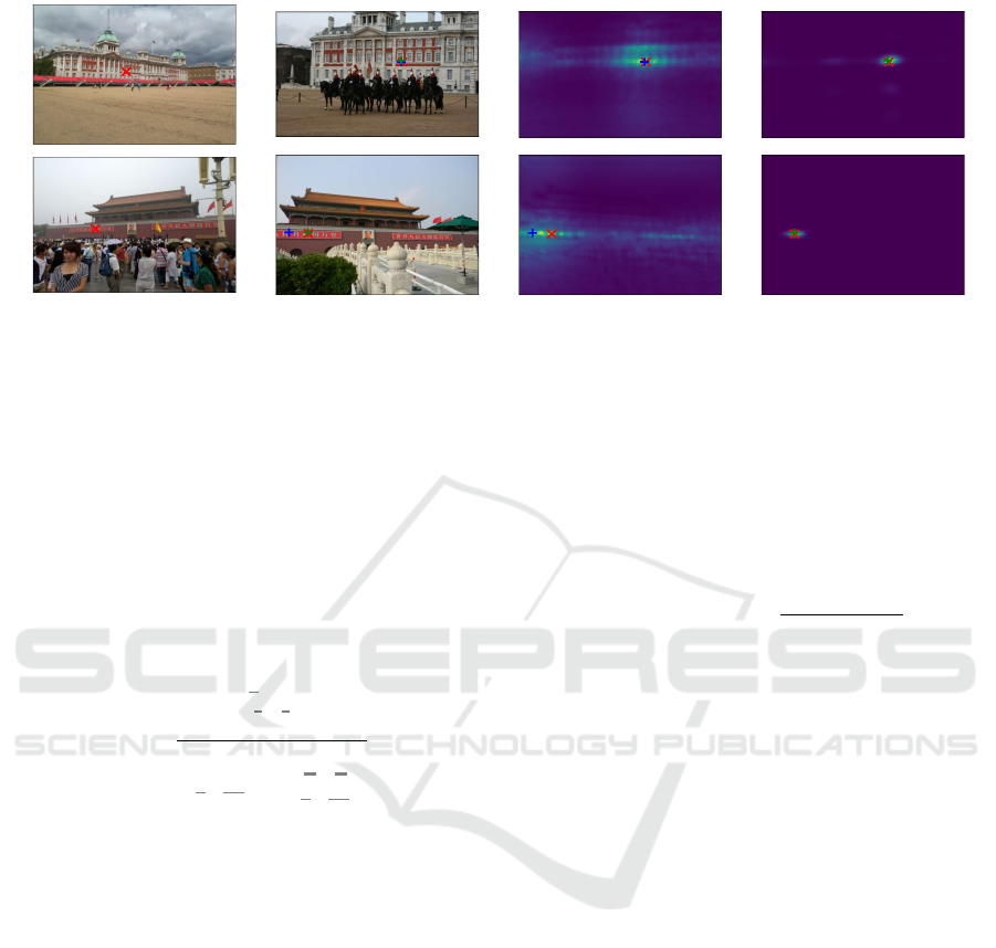
Source Image Target Image Visio-positional map Positional map
Figure 4: Visualization - Structured attention. The visio-positional and positional maps are computed before the output
cross-attention. Red crosses represent the ground-truth correspondences. Blue and Green crosses are the maxima of the
visio-positional and positional maps, respectively. One can see that the visio-positional maps are highly multimodal (i.e.,
sensitive to repetitive structures) while the positional maps are almost unimodal.
3.4 Structured Attention
At the end of the feature extraction stage, the upper
half of each vector is visual features, while the lower
half is positional encodings. In each attention layer
(input cross-attention, self-attention and output cross-
attention), we found it important to structure the lin-
ear transformation matrices W
o,h
and W
v,h
to constrain
the lower half of each output vector to only contain a
linear transformation of the positional encodings:
D×D
H
z}|{
W
o,h
=

D
2
×D
H
z}| {
W
o,h,up
0
|{z}
D
2
×
D
H
2
| W
o,h,low
| {z }
D
2
×
D
H
2

. (4)
The matrices W
v,h
and the fully connected layers
within the MLP (at the end of each attention mod-
ule) are structured the exact same way. Consequently,
throughout the network, the lower half of each latent
vector only contains transformations of positional en-
codings, but no visual feature.
In Figure 4 we propose a visualization of two dif-
ferent correspondence maps before the output cross-
attention.
The first map is produced using the first 128 di-
mensions of the feature representation and contains
high-level visio-positional features. The second map
is produced using the 128 last dimensions of the fea-
ture representation and contains only positional en-
codings. By building these distinct correspondence
maps we can observe that while the visio-positional
representation is sensitive to repetitive structures, the
purely positional representation tends to be only acti-
vated in the areas neighbouring the match.
3.5 Loss
At training time, we use a cross-entropy (CE) loss
function (Germain et al., 2020) on each correspon-
dence map C
t,i
in order to maximise its score at the
ground truth location p
t,i
:
CE(C
t,i
, p
t,i
) = −ln

exp C
t,i
(p
t,i
)
∑
q
exp C
t,i
(q)

. (5)
3.6 Refinement
The previously described architecture produces
coarse correspondence maps of resolution 1/4. Thus
the predicted correspondents
{
ˆ
p
t,i
}
i=1...L
need to be
refined. To do so, we simply use a second siamese
CNN that outputs dense source and target features at
full resolution. For each 2D query location p
s,i
, a cor-
respondence map is computed on a window of size
11 centered around the coarse prediction. The pre-
dicted 2D correspondent location
ˆ
p
t,i
is defined as the
argmax of this correspondence map. This refinement
network is trained separately using the same cross-
entropy loss eq. 5. Technical details are provided in
the appendix.
4 EXPERIMENTS
In these experiments, we focus on evaluating six SDF
networks (LoFTR (Sun et al., 2021), QuadTree (Tang
et al., 2022), ASpanFormer (Chen et al., 2022), 3DG-
STFM (Mao et al., 2022), MatchFormer (Wang et al.,
2022), TopicFM (Giang et al., 2023)) and our pro-
posed architecture SAM. In all the following Tables,
best and second best results are respectively bold and
underlined.
Are Semi-Dense Detector-Free Methods Good at Matching Local Features?
39

Table 1: Evaluation on MegaDepth1500 (Sarlin et al., 2020). We report Matching Accuracy (6) for several thresholds η,
computed on the set of all the semi-dense query locations (source grid with stride 8) with available ground truth correspon-
dents (MA), and on a subset containing only query locations that are within a textured region of the source image (MA
text
).
Concerning the pose estimation metrics, we report the classical AUC at 5, 10 and 20 degrees. The proposed SAM method
outperforms SDF methods in terms of pose estimation, while SDF methods are significantly better in terms of MA. However,
when uniform regions are ignored (MA
text
), SAM often surpasses SDF methods. These results highlight a strong correlation
between the ability to establish precise correspondences in textured regions and the accuracy of the resulting estimated pose.
Method
Matching Accuracy (MA) (6) ↑
Matching Accuracy Pose estimation on
on textured regions (MA
text
) (6) ↑ 1/8 grid (AUC) ↑
η=1 η=2 η=3 η=5 η=10 η=20 η=1 η=2 η=3 η=5 η=10 η=20 @5
o
@10
o
@20
o
LoFTR (Sun et al., 2021) 49.7 73.2 81.6 87.4 90.5 91.8 55.3 75.2 81.6 86.9 89.9 91.9 52.8 69.2 82.0
MatchFormer (Wang et al., 2022) 51.1 73.4 81.0 86.9 89.5 90.9 56.5 75.6 81.8 87.1 89.6 90.9 52.9 69.7 82.0
TopicFM (Giang et al., 2023) 51.4 75.4 83.7 89.9 92.9 93.5 59.8 77.6 84.8 90.4 92.9 93.7 54.1 70.1 81.6
3DG-STFM(Mao et al., 2022) 51.6 73.7 80.7 86.4 89.0 90.7 57.0 75.8 81.8 86.8 88.8 90.5 52.6 68.5 80.0
ASpanFormer (Chen et al., 2022) 52.0 76.2 84.5 90.7 93.7 94.8 62.2 80.3 85.9 91.0 93.7 94.7 55.3 71.5 83.1
LoFTR+QuadTree (Tang et al., 2022) 51.6 75.9 84.1 90.2 93.1 94.0 61.7 79.9 85.5 90.5 93.3 94.1 54.6 70.5 82.2
SAM (ours) 48.5 70.4 78.0 83.0 85.4 86.4 67.9 83.8 87.3 90.6 93.6 95.2 55.8 72.8 84.2
Table 2: Evaluation on HPatches (Balntas et al., 2017). We report Matching Accuracy (6) for several thresholds η, computed
on the set of all the semi-dense query locations (source grid with stride 8) with available ground truth correspondents (MA),
and on a subset containing only query locations that are within a textured region of the source image (MA
text
). Concerning the
homography estimation metrics, we report the classical AUC at 3, 5 and 10 pixels. The proposed SAM method is on par with
SDF methods in terms of homography estimation, while SDF methods are significantly better in terms of MA. However, when
uniform regions are ignored (MA
text
), SAM matches SDF performances. These results highlight a strong correlation between
the ability to establish precise correspondences in textured regions and the accuracy of the resulting estimated homography.
Method
Matching Accuracy Matching Accuracy on Homography estimation
(MA) (6) ↑ textured regions (MA
text
) (6) ↑ (AUC) ↑
η=3 η=5 η=10 η=3 η=5 η=10 @3px @5px @10px
LoFTR (Sun et al., 2021) 66.8 74.3 77.3 67.6 75.3 78.4 65.9 75.6 84.6
MatchFormer (Wang et al., 2022) 66.2 74.9 78.2 67.7 75.8 79.1 65.0 73.1 81.2
TopicFM (Giang et al., 2023) 72.7 85.0 87.5 74.0 86.0 88.5 67.3 77.0 85.7
3DG-STFM(Mao et al., 2022) 64.9 75.1 78.2 66.2 74.3 77.6 64.7 73.1 81.0
ASpanFormer (Chen et al., 2022) 76.2 86.2 88.7 73.9 85.8 88.4 67.4 76.9 85.6
LoFTR+QuadTree (Tang et al., 2022) 70.2 83.1 85.9 73.5 84.3 86.9 67.1 76.1 85.3
SAM (ours) 62.4 70.9 74.2 73.4 86.6 89.3 67.1 76.9 85.9
Table 3: Evaluation on ETH3D (Sch
¨
ops et al., 2019) for different frame interval sampling rates r. We report Matching
Accuracy (6) for several thresholds η, computed on the set of all the semi-dense query locations (source grid with stride
8) with available ground truth correspondents (MA). For ETH3D, ground truth correspondents are based on structure from
motion tracks. Consequently, the MA already ignores untextured regions of the source images which explains why SAM is
able to outperform SDF methods.
Method
Matching Accuracy (MA) (6) ↑
r = 3 r = 7 r = 15
η=1 η=2 η=3 η=5 η=10 η=1 η=2 η=3 η=5 η=10 η=1 η=2 η=3 η=5 η=10
LoFTR (Sun et al., 2021) 44.8 76.5 88.4 97.0 99.4 39.7 73.1 87.6 95.9 98.5 33.3 66.2 84.8 92.5 96.3
MatchFormer (Wang et al., 2022) 45.5 77.1 89.2 97.2 99.7 40.4 73.8 87.8 96.6 99.0 34.2 66.7 84.9 93.5 97.0
TopicFM (Giang et al., 2023) 45.1 76.9 89.0 97.2 99.6 39.9 73.5 87.9 96.4 99.0 33.8 66.4 85.0 92.8 96.5
3DG-STFM(Mao et al., 2022) 43.9 76.3 88.0 96.9 99.3 39.3 72.7 87.4 95.5 98.3 32.4 65.7 84.7 92.0 96.0
ASpanFormer (Chen et al., 2022) 45.8 77.6 89.6 97.8 99.8 40.6 73.8 88.1 96.8 99.0 34.3 66.8 85.3 93.9 97.3
LoFTR+QuadTree (Tang et al., 2022) 45.9 77.5 89.5 97.8 99.7 40.8 74.0 88.3 97.0 99.2 34.5 66.8 85.4 94.0 97.3
SAM (ours) 53.4 79.9 91.5 98.0 99.8 48.6 78.6 91.7 98.2 99.4 40.1 70.2 87.8 95.4 97.8
VISAPP 2024 - 19th International Conference on Computer Vision Theory and Applications
40

Implementations. For each network, we employ
the code and weights (trained on MegaDepth) made
available by the authors. Concerning SAM, we train it
similarly to the SDF networks on MegaDepth (Li and
Snavely, 2018), during 100 hours, on four GeForce
GTX 1080 Ti (11GB) GPUs (see the appendix for de-
tails). Our code will be made available.
Query Locations. Concerning SDF methods, the
query locations are defined as the source grid loca-
tions using a stride of 8. Thus, in order to be able
to compare the performances of SAM against such
methods, we use the exact same query locations. To
do so (recall that SAM was trained with L = 1024
query locations), we simply shuffle the source grid lo-
cations (with stride 8) and feed them to SAM by batch
of size 1024 (the CNN features are cached making the
processing of each minibatch very efficient).
Evaluation Criteria. Regarding the pose and ho-
mography estimation metrics, we use the classical
AUC metrics for each dataset. Thus in each Table, the
pose/homography results we obtained for SDF meth-
ods (we re-evaluated each method) are the same as
the results published in the respective papers. Con-
cerning SAM, the correspondences are classically fil-
tered (similarly to what SDF methods do) before the
pose/homography estimator using a simple Mutual
Nearest Neighbor with a threshold of 5 pixels.
In order to evaluate the ability of each method to
establish correspondences, we consider the Matching
Accuracy (MA) as in (Truong et al., 2020), i.e., the
average on all images of the ratio of correct matches,
for different pixel error thresholds (η):
MA(η) =
1
K
K
∑
k=1
∑
L
k
i=1
h



ˆ
p
t
k
,i
− p
GT
t
k
,i



2
< η
i
L
k
, (6)
where K is the number of pairs of images, L
k
is the
number of ground truth correspondences available for
the image pair #k and [·] is the Iverson bracket. We
refer to this metric as MA and not ”Percentage of Cor-
rect Keypoints” because we found this term mislead-
ing in cases where the underlying ground truth cor-
respondences are not based on keypoints, as it is the
case in MegaDepth and HPatches.
We also propose to introduce the Matching Ac-
curacy in textured regions (MA
text
) that consists in
ignoring, in eq. (6), ground truth correspondences
whose query location is within a low-contrast region
of the source image, i.e., an almost uniform region of
the source image.
Note that SAM’s MNN (and the MNN of SDF
methods) is only used for the pose/homography es-
timation, i.e., it is not used to compute matching ac-
curacies, otherwise the set of correspondences would
not be the same for each method.
4.1 Evaluation on MegaDepth
We consider the MegaDepth1500 (Sarlin et al., 2020)
benchmark. We use the exact same settings as those
used by SDF methods, such as an image resolution
of 1200. The results are provided in Table 1. We re-
port Matching Accuracy (6), for several thresholds η,
computed on the set of all the semi-dense query loca-
tions (source grid with stride 8) with available ground
truth correspondents (MA). The ground truth corre-
spondents are obtained using the available depth maps
and camera poses. Consequently, many query loca-
tions located in untextured regions have a ground truth
correspondent. Thus, we also report the matching
accuracy computed only on query locations that are
within a textured region of the source image (MA
text
).
Concerning the pose estimation metrics, we report the
classical AUC at 5, 10 and 20 degrees. The proposed
SAM method outperforms SDF methods in terms of
pose estimation, while SDF methods are significantly
better in terms of MA. However, when uniform re-
gions are ignored (MA
text
), SAM often surpasses SDF
methods. These results highlight a strong correla-
tion between the ability to establish precise corre-
spondences in textured regions and the accuracy of
the resulting estimated pose.
In Figure 5, we report qualitative results that visu-
ally illustrate the previous findings.
4.2 Evaluation on HPatches
We evaluate the different architectures on
HPatches (Balntas et al., 2017) (see Table 2).
We use the exact same settings as those used by
SDF methods. We report Matching Accuracy (6)
for several thresholds η, computed on the set of all
the semi-dense query locations (source grid with
stride 8) with available ground truth correspondents
(MA). The ground truth correspondents are obtained
using the available homography matrices. Conse-
quently, many query locations located in untextured
regions have a ground truth correspondent. Thus,
we also report the matching accuracy computed
only on query locations that are within a textured
region of the source image (MA
text
). Concerning
the homography estimation metrics, we report the
classical AUC at 3, 5 and 10 pixels. The proposed
SAM method is on par with SDF methods in terms
of homography estimation, while SDF methods are
significantly better in terms of MA. However, when
uniform regions are ignored (MA
text
), SAM matches
SDF performances. These results highlight a strong
correlation between the ability to establish precise
correspondences in textured regions and the accuracy
Are Semi-Dense Detector-Free Methods Good at Matching Local Features?
41

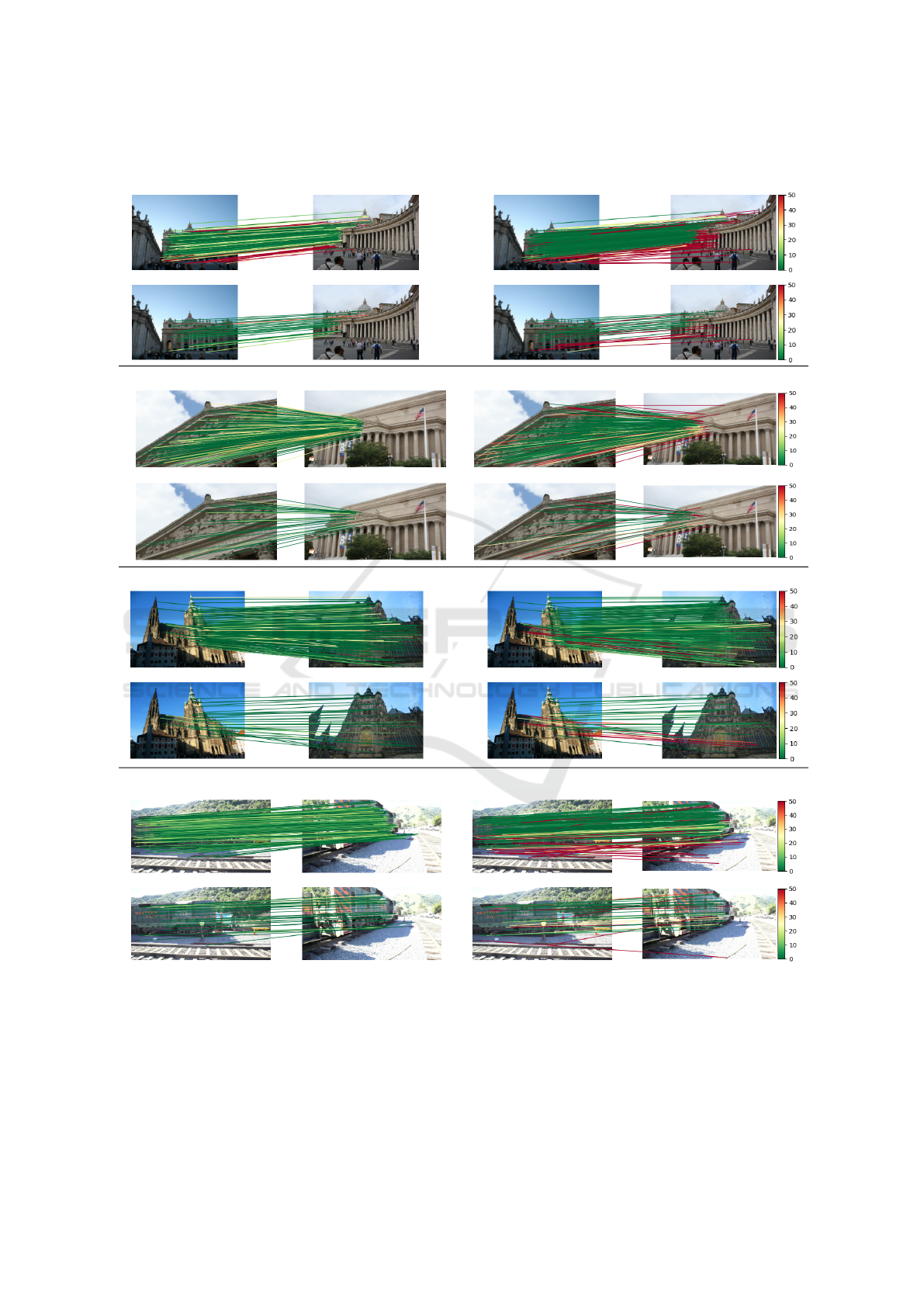
SAM (ours) LoFTR+QuadTree (Tang et al., 2022)
MA@2=60.6 MA
text
@2=84.0 errR=2.1’ errT=5.4’ MA@2=62.8 MA
text
@2=64.0 errR=5.5’ errT=22.4’
MA@2=62.3 MA
text
@2=81.1 errR=1.9’ errT=5.5’ MA@2=66.2 MA
text
@2=67.5 errR=2.1’ errT=9.4’
MA@2=79.0 MA
text
@2=83.1 errR=1.5’ errT=3.9’ MA@2=79.9 MA
text
@2=78.7 errR=2.0’ errT=6.4’
MA@5=69.1 MA
text
@5=78.0 errR=3.8’ errT=15.4’ MA@5=70.7 MA
text
@5=72.1 errR=4.9’ errT=19.6’
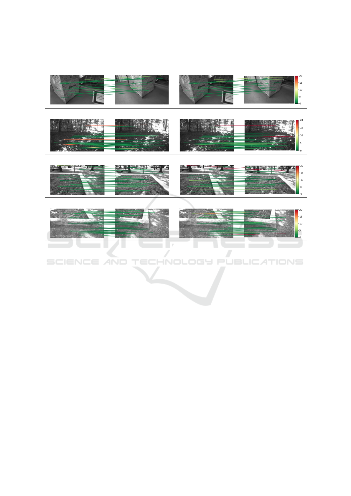
Figure 5: Qualitative results on MegaDepth1500. For each image pair: (top row) Visualization of established correspon-
dences used to compute the MA, (bottom row) Visualization of established correspondences used to compute the MA
text
.
Line colors indicate the distance in pixels with respect to the ground truth correspondent.
VISAPP 2024 - 19th International Conference on Computer Vision Theory and Applications
42

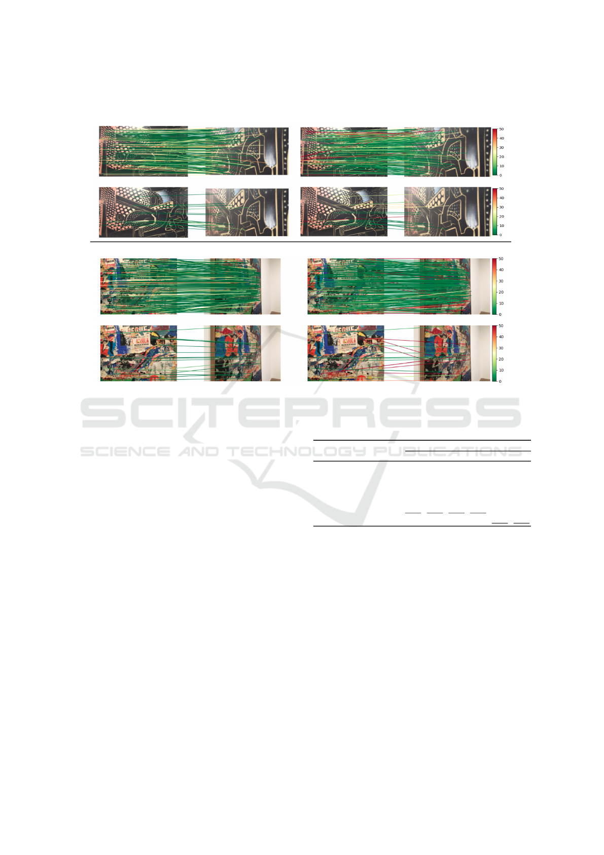
SAM (ours) LoFTR+QuadTree (Tang et al., 2022)
MA@5=69.7 MA
text
@5=88.6 AUC@5=77.4 MA@5=72.1 MA
text
@5=76.6 AUC@5=76.1
MA@5=74.4 MA
text
@5=86.2 AUC@5=81.5 MA@5=77.1 MA
text
@5=42.8 AUC@5=75.9
Figure 6: Qualitative results on HPatches. Line colors indicate the distance in pixels to the ground truth correspondent.
of the resulting estimated homography.
In Figure 6, we report qualitative results that visu-
ally illustrate the previous findings.
4.3 Evaluation on ETH3D
We evaluate the different networks on several se-
quences of the ETH3D dataset (Sch
¨
ops et al., 2019)
as proposed in (Truong et al., 2020). Different frame
interval sampling rates r are considered. As the rate
r increases, the overlap between the image pairs re-
duces, hence making the matching problem more dif-
ficult. The results are provided in Table 3. We re-
port Matching Accuracy (6) for several thresholds η,
computed on the set of all the semi-dense query loca-
tions (source grid with stride 8) with available ground
truth correspondents (MA). For ETH3D, ground truth
correspondents are based on structure from motion
tracks. Consequently, the MA ignores untextured re-
gions of the source images which explains why SAM
is able to outperform SDF methods in terms of MA.
In Figure 7, we report qualitative results that illus-
trate the accuracy of the proposed SAM method.
4.4 Ablation Study
In Table 4, we propose an ablation study of SAM to
evaluate the impact of each part of our architecture.
Table 4: Ablation study of proposed SAM method
(MegaDepth validation set).
Method
MA
text
↑
η=1 η=2 η=5 η=10 η=20 η=50
Siamese CNN 0.029 0.112 0.436 0.581 0.622 0.687
+ Input CA and SA (x16) 0.137 0.321 0.671 0.734 0.767 0.822
+ Learned LV and output CA 0.132 0.462 0.823 0.871 0.898 0.935
+ PE concatenated 0.121 0.419 0.796 0.868 0.902 0.939
+ Structured AM 0.140 0.487 0.857 0.902 0.922 0.947
+ Refinement (Full model) 0.673 0.791 0.870 0.902 0.921 0.946
This study is performed on MegaDepth validation
scenes. Starting from a standard siamese CNN, we
show that a significant gain in performance can sim-
ply be obtained with the input cross-attention layer
(here the PE is added and not concatenated) and self-
attention layers. We then add learned latent vectors
(LV) in the latent space and use an output cross-
attention which again significantly improves the per-
formance. Concatenating the positional encoding in-
formation instead of adding it to the visual features
reduces the matching accuracy at η = 2 and η = 5.
However, combining it with structured attention leads
to a significant improvement in terms of MA. Finally,
as expected, the refinement step improves the match-
ing accuracy for small pixel error thresholds.
Are Semi-Dense Detector-Free Methods Good at Matching Local Features?
43

SAM (ours) LoFTR+QuadTree (Tang et al., 2022)
MA
text
@2=75.0 MA
text
@2=68.8
MA
text
@2=65.4 MA
text
@2=61.5
MA
text
@2=80.0 MA
text
@2=68.0
MA
text
@2=87.2 MA
text
@2=69.2
Figure 7: Qualitative results on ETH3D. Line colors indicate the distance in pixels to the ground truth correspondent.
5 CONCLUSION
We proposed a novel Structured Attention-based im-
age Matching architecture (SAM). The flexibility of
this novel architecture allowed us to fairly compare it
against SDF methods, i.e., in all the experiments we
used the same query locations (source grid with stride
8). The experiments highlighted a counter-intuitive
result on two datasets (MegaDepth and HPatches):
on the one hand SAM either outperforms or is on
par with SDF methods in terms of pose/homography
estimation metrics, but on the other hand SDF ap-
proaches are significantly better than SAM in terms of
Matching Accuracy (MA). Here the MA is computed
on all the semi-dense locations of the source image
with available ground truth correspondent, which in-
cludes both textured and uniform regions. We pro-
posed to limit the computation of the matching ac-
curacy to textured regions, and showed that in this
case SAM often surpasses SDF methods. These find-
ings highlighted a strong correlation between the abil-
ity to establish precise correspondences in textured
regions and the accuracy of the resulting estimated
pose/homography. We also evaluated the aforemen-
tioned methods on ETH3D which confirmed, on a
third dataset, that SAM has a strong ability to estab-
lish correspondences in textures regions. We finally
performed an ablation study of SAM to demonstrate
that each part of the architecture is important to obtain
such a strong matching capacity.
REFERENCES
Arnold, E., Wynn, J., Vicente, S., Garcia-Hernando, G.,
Monszpart,
´
A., Prisacariu, V. A., Turmukhambetov,
D., and Brachmann, E. (2022). Map-free visual relo-
calization: Metric pose relative to a single image. In
ECCV.
Balntas, V., Lenc, K., Vedaldi, A., and Mikolajczyk, K.
(2017). Hpatches: A benchmark and evaluation of
handcrafted and learned local descriptors. In CVPR.
Chen, H., Luo, Z., Zhou, L., Tian, Y., Zhen, M., Fang, T.,
McKinnon, D., Tsin, Y., and Quan, L. (2022). Aspan-
former: Detector-free image matching with adaptive
span transformer. In ECCV.
Dusmanu, M., Rocco, I., Pajdla, T., Pollefeys, M., Sivic,
J., Torii, A., and Sattler, T. (2019). D2-net: A train-
VISAPP 2024 - 19th International Conference on Computer Vision Theory and Applications
44

able CNN for joint description and detection of local
features. In CVPR.
Edstedt, J., Athanasiadis, I., Wadenb
¨
ack, M., and Felsberg,
M. (2023). Dkm: Dense kernelized feature match-
ing for geometry estimation. In Proceedings of the
IEEE/CVF Conference on Computer Vision and Pat-
tern Recognition, pages 17765–17775.
Germain, H., Bourmaud, G., and Lepetit, V. (2020).
S2DNet: learning image features for accurate sparse-
to-dense matching. In ECCV.
Germain, H., Lepetit, V., and Bourmaud, G. (2021). Neural
reprojection error: Merging feature learning and cam-
era pose estimation. In CVPR.
Germain, H., Lepetit, V., and Bourmaud, G. (2022). Visual
correspondence hallucination. In ICLR.
Giang, K. T., Song, S., and Jo, S. (2023). TopicFM: Robust
and interpretable feature matching with topic-assisted.
In AAAI.
Heinly, J., Sch
¨
onberger, J. L., Dunn, E., and Frahm, J.-M.
(2015). Reconstructing the World* in Six Days *(as
Captured by the Yahoo 100 Million Image Dataset).
In CVPR.
Jaegle, A., Borgeaud, S., Alayrac, J.-B., Doersch, C.,
Ionescu, C., Ding, D., Koppula, S., Zoran, D., Brock,
A., Shelhamer, E., Henaff, O. J., Botvinick, M., Zis-
serman, A., Vinyals, O., and Carreira, J. (2022). Per-
ceiver IO: A general architecture for structured inputs
& outputs. In ICLR.
Jaegle, A., Gimeno, F., Brock, A., Vinyals, O., Zisserman,
A., and Carreira, J. (2021). Perceiver: General per-
ception with iterative attention. In ICML.
Jin, Y., Mishkin, D., Mishchuk, A., Matas, J., Fua, P., Yi,
K. M., and Trulls, E. (2020). Image Matching across
Wide Baselines: From Paper to Practice. IJCV.
Katharopoulos, A., Vyas, A., Pappas, N., and Fleuret, F.
(2020). Transformers are RNNs: Fast autoregressive
transformers with linear attention. In ICML.
Li, X., Han, K., Li, S., and Prisacariu, V. (2020). Dual-
resolution correspondence networks. NeurIPS.
Li, Z. and Snavely, N. (2018). Megadepth: Learning single-
view depth prediction from internet photos. In CVPR.
Lin, T.-Y., Doll
´
ar, P., Girshick, R., He, K., Hariharan, B.,
and Belongie, S. (2017). Feature pyramid networks
for object detection. In CVPR.
Lowe, D. G. (1999). Object recognition from local scale-
invariant features. In ICCV.
Mao, R., Bai, C., An, Y., Zhu, F., and Lu, C. (2022). 3DG-
STFM: 3D geometric guided student-teacher feature
matching. In ECCV.
Ni, J., Li, Y., Huang, Z., Li, H., Bao, H., Cui, Z., and Zhang,
G. (2023). PATS: Patch area transportation with sub-
division for local feature matching. In Proceedings
of the IEEE/CVF Conference on Computer Vision and
Pattern Recognition, pages 17776–17786.
Ono, Y., Trulls, E., Fua, P., and Yi, K. M. (2018). LF-Net:
learning local features from images. NeurIPS.
Revaud, J., De Souza, C., Humenberger, M., and Weinza-
epfel, P. (2019). R2D2: reliable and repeatable detec-
tor and descriptor. NeurIPS.
Rocco, I., Arandjelovi
´
c, R., and Sivic, J. (2020a). Efficient
neighbourhood consensus networks via submanifold
sparse convolutions. In ECCV.
Rocco, I., Cimpoi, M., Arandjelovi
´
c, R., Torii, A., Pajdla,
T., and Sivic, J. (2018). Neighbourhood consensus
networks. NeurIPS.
Rocco, I., Cimpoi, M., Arandjelovi
´
c, R., Torii, A., Pajdla,
T., and Sivic, J. (2020b). NCNet: neighbourhood
consensus networks for estimating image correspon-
dences. PAMI.
Sarlin, P.-E., DeTone, D., Malisiewicz, T., and Rabinovich,
A. (2020). Superglue: Learning feature matching with
graph neural networks. In CVPR.
Sarlin, P.-E., Dusmanu, M., Sch
¨
onberger, J. L., Speciale,
P., Gruber, L., Larsson, V., Miksik, O., and Pollefeys,
M. (2022). LaMAR: Benchmarking Localization and
Mapping for Augmented Reality. In ECCV.
Sattler, T., Torii, A., Sivic, J., Pollefeys, M., Taira, H., Oku-
tomi, M., and Pajdla, T. (2017). Are large-scale 3D
models really necessary for accurate visual localiza-
tion? In CVPR.
Sch
¨
onberger, J. L. and Frahm, J.-M. (2016). Structure-
from-motion revisited. In CVPR.
Sch
¨
ops, T., Sattler, T., and Pollefeys, M. (2019). BAD
SLAM: Bundle adjusted direct RGB-D SLAM. In
CVPR.
Strasdat, H., Davison, A. J., Montiel, J. M., and Konolige,
K. (2011). Double window optimisation for constant
time visual slam. In ICCV.
Sun, J., Shen, Z., Wang, Y., Bao, H., and Zhou, X.
(2021). LoFTR: detector-free local feature matching
with transformers. In CVPR.
Sv
¨
arm, L., Enqvist, O., Kahl, F., and Oskarsson, M. (2017).
City-scale localization for cameras with known verti-
cal direction. PAMI.
Taira, H., Okutomi, M., Sattler, T., Cimpoi, M., Pollefeys,
M., Sivic, J., Pajdla, T., and Torii, A. (2018). In-
Loc: Indoor visual localization with dense matching
and view synthesis. In CVPR.
Tang, S., Zhang, J., Zhu, S., and Tan, P. (2022). Quadtree
attention for vision transformers. In ICLR.
Truong, P., Danelljan, M., and Timofte, R. (2020). Glu-
net: Global-local universal network for dense flow and
correspondences. In CVPR.
Truong, P., Danelljan, M., Van Gool, L., and Timofte, R.
(2021). Learning accurate dense correspondences and
when to trust them. In CVPR.
Vaswani, A., Shazeer, N., Parmar, N., Uszkoreit, J., Jones,
L., Gomez, A. N., Kaiser, Ł., and Polosukhin, I.
(2017). Attention is all you need. NeurIPS.
Wang, Q., Zhang, J., Yang, K., Peng, K., and Stiefelha-
gen, R. (2022). Matchformer: Interleaving attention
in transformers for feature matching. In ACCV.
Wang, W., Xie, E., Li, X., Fan, D.-P., Song, K., Liang, D.,
Lu, T., Luo, P., and Shao, L. (2021). Pyramid vision
transformer: A versatile backbone for dense predic-
tion without convolutions. In ICCV.
Xie, E., Wang, W., Yu, Z., Anandkumar, A., Alvarez, J. M.,
and Luo, P. (2021). Segformer: Simple and efficient
Are Semi-Dense Detector-Free Methods Good at Matching Local Features?
45

design for semantic segmentation with transformers.
NeurIPS.
Yi, K. M., Trulls, E., Lepetit, V., and Fua, P. (2016). LIFT:
Learned invariant feature transform. In ECCV.
Zhang, Z., Sattler, T., and Scaramuzza, D. (2021). Refer-
ence pose generation for long-term visual localization
via learned features and view synthesis. IJCV.
Zhou, Q., Sattler, T., and Leal-Taixe, L. (2021). Patch2Pix:
Epipolar-guided pixel-level correspondences. In
CVPR.
Zhu, S. and Liu, X. (2023). Pmatch: Paired masked image
modeling for dense geometric matching. In Proceed-
ings of the IEEE/CVF Conference on Computer Vision
and Pattern Recognition, pages 21909–21918.
APPENDIX
SAM Architecture. Each attention layer in SAM is
a classical series of softmax attention, normalization,
MLP and normalization layers with residual connec-
tions, except for the ”output” cross-attention where
we removed the MLP, the last normalization and the
residual connection.
We empirically choose a combination of 16 self-
attention layers and 128 vectors in the learned latent
space. We found this combination to be a good trade-
off between performance and computational cost.
Backbone Description. We use a modified ResNet-
18 as our feature extraction backbone. We extract the
feature map after the last ResBlock in which we re-
moved the last ReLU. The features are reduced to
1
4
th
of the image resolution (3 × H × W ) by apply-
ing a stride of 2 in the first and third layer. The fea-
ture representation built by the backbone is of size
128 ×
1
4
H ×
1
4
W .
Refinement Description. The previous CNN back-
bone is used for refinement. We simply added a FPN
(Feature Pyramid Network) module to extract the fea-
ture maps after the first convolutional layer and each
ResNet layer. It leaves us with a feature map of size
128 × H × W on which the refinement stage is per-
formed.
Structured Attention. In our implementation, D =
256, we use 8 heads, thus D
H
= 32.
Training Details. The first part of the model to be
trained is the refinement model (CNN+FPN). It is
trained during 50 hours on 4 Nvidia GTX1080 Ti
GPUs using Adam optimizer, a constant learning rate
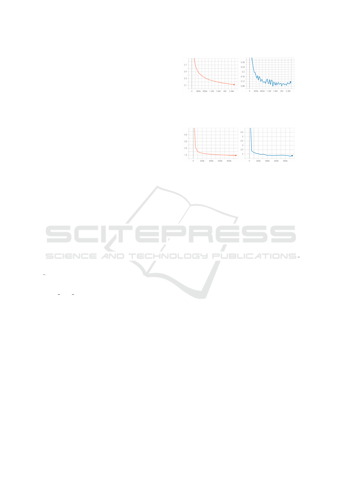
Figure 8: Training (left) and Validation (right) loss for
refinement ResNet-18+FPN. x-axis represent the number
of mini-batches seen by the model and y-axis the cross-
entropy value.
Figure 9: Training (left) and Validation (right) loss for
SAM. x-axis represent the number of mini-batches seen by
the model and y-axis the cross-entropy value.
of 10
−3
and a batch size of 1 (Figure 8). We min-
imize the cross-entropy of the full resolution corre-
spondence maps produced using the FPN.
The CNN backbone of SAM is initialized with the
weights of the previously trained network. We train
SAM for 100 hours. The same setup with 4 Nvidia
GTX1080 Ti GPUs, Adam optimizer and a batch size
of 1 is used. Concerning the learning rate schedule,
we use a linear warm-up of 5000 steps (from 0 to
10
−4
) and then an exponential decay (towards 10
−5
)
(Figure 9). We minimize the cross-entropy of the
1
4
resolution correspondence maps produced by SAM.
VISAPP 2024 - 19th International Conference on Computer Vision Theory and Applications
46