Improving the Sum-of-Cost Methods for Reduction-Based Multi-Agent

Pathﬁnding Solvers

Roland Kaminski

, Torsten Schaub

, Klaus Strauch

and Ji

Svancara

University of Potsdam, Germany

Charles University, Czech Republic

Keywords:

Multi-Agent Pathﬁnding, Sum of Costs, Reduction-Based Algorithm.

Abstract:

Multi-agent pathﬁnding is the task of guiding a group of agents through a shared environment while preventing

collisions. This problem is highly relevant in various real-life scenarios, such as warehousing, robotics,

navigation, and computer games. Depending on the context in which the problem is applied, we may have

speciﬁc criteria for the quality of a solution, expressed as a cost function. The most common cost functions

are the makespan and sum-of-cost. Minimizing either of them is computationally challenging, leading to the

development of numerous approaches for solving multi-agent pathﬁnding. In this paper, we explore reduction-

based solving under the sum-of-cost objective. We introduce a reduction to answer set programming (ASP)

using two existing approaches for sum-of-cost minimization, originally introduced for a reduction to Boolean

satisﬁability (SAT). We propose several enhancements and use the Clingo ASP system to implement them.

Experiments show that these enhancements signiﬁcantly improve performance. Particularly, the performance

on larger maps increases in comparison to the original variants.

1 INTRODUCTION

Multi-agent pathﬁnding (MAPF) is the task of guid-

ing a group of agents through a shared environment

while preventing collisions. This problem is highly

relevant in various real-life scenarios, such as ware-

housing (Ma et al., 2017), robotics (Bennewitz et al.,

2002), navigation (Dresner and Stone, 2008), and com-

puter games (Wang and Botea, 2008).

Depending on the context, we may have speciﬁc

criteria for the quality of the solution, expressed as a

cost function. The most commonly used cost functions

are makespan (i.e., minimizing the time for all agents

to reach their destinations) and sum-of-cost (i.e., min-

imizing the total number of actions performed by all

agents) (Stern et al., 2019). Each of these cost func-

tions serves a practical purpose: makespan optimiza-

tion focuses on minimizing the overall task completion

time, even if it means some agents perform more ac-

tions. On the other hand, sum-of-cost optimization

aims to reduce the total number of actions, which can

be associated with minimizing energy consumption.

Minimizing either of these cost functions is compu-

tationally challenging (Yu and LaValle, 2013), leading

to the development of numerous approaches for opti-

mally solving MAPF problems (Boyarski et al., 2015;

Lam et al., 2019; Surynek et al., 2016; Sharon et al.,

2011). In this paper, we explore reduction-based solv-

ing under the sum-of-cost objective. We review the two

existing optimization approaches – iterative (Surynek

et al., 2016) and jump (Bart

ak and Svancara, 2019),

both originally developed for reductions to Boolean

satisﬁability (SAT). Then, we introduce a reduction to

answer set programming (ASP) (Gebser et al., 2012;

Lifschitz, 2019) and adapt the two optimization ap-

proaches. Furthermore, we propose several enhance-

ments to the jump approach and leverage the multi-

shot solving capabilities and inbuilt optimization strate-

gies of the Clingo (Kaminski et al., 2023) ASP system

to implement them. The ﬁrst enhancement is the use of

techniques from the iterative approach to quickly ﬁnd

an initial solution. Next, we improve on the ﬁrst en-

hancement by increasing the iteration step size. Finally,

we show unsatisﬁable-core based optimization dramat-

ically improves performance. We present a series of

experiments demonstrating that these enhancements

indeed lead to performance gains. Particularly, the per-

formance on larger maps is increased in comparison

to the original variants.

264

Kaminski, R., Schaub, T., Strauch, K. and Švancara, J.

Improving the Sum-of-Cost Methods for Reduction-Based Multi-Agent Pathﬁnding Solvers.

DOI: 10.5220/0012353500003636

Paper published under CC license (CC BY-NC-ND 4.0)

In Proceedings of the 16th International Conference on Agents and Artiﬁcial Intelligence (ICAART 2024) - Volume 1, pages 264-271

ISBN: 978-989-758-680-4; ISSN: 2184-433X

2 BACKGROUND

The multi-agent pathﬁnding problem (MAPF) (Stern

et al., 2019) is a pair

(G, A)

, where

is an undi-

rected graph

G = (V, E)

and

is a list of agents

A = (a

, . . . , a

)

. Each agent

∈ A

is associated with

a start vertex s

∈ V and a goal vertex g

∈ V.

Time is considered discrete; between two consecu-

tive timesteps, an agent can either move to an adjacent

vertex (move action) or stay at its current vertex (wait

action). The movement of an agent is captured by its

path. A path

of agent

is a list of vertices that

starts at

and ends at

. Let

(t)

be the vertex (i.e.,

location) of

at timestep

according to

. Therefore,

(0) = s

(|π

|) = g

, and for all timesteps

t < |π

(π

(t), π

(t + 1)) ∈ E

(t) = π

(t + 1)

, that is, at

each timestep agent

either moves along an edge or

waits at a vertex, respectively.

As there are several agents, we are interested in the

interaction of pairs of paths of distinct agents. There

is a conﬂict between paths

and

at timestep

(t) = π

(t)

(vertex conﬂict) or

(t) = π

(t + 1)

and

(t) = π

(t + 1)

(swapping conﬂict). A plan

is a

list of

paths

Π = (π

, . . . , π

)

, one for each agent. A

solution is a conﬂict-free plan, i.e., a plan

where no

two paths of distinct agents have conﬂicts.

A solution is optimal if it has the lowest cost among

all possible solutions. The cost

C(π

)

of path

equals

the number of actions performed in

until the last

arrival at

, not counting any subsequent wait ac-

tions. Formally,

C(π

) = max({0 < t ≤ |π

| | π

(t) =

, π

(t −1) ̸= g

}∪{0})

. Note that waiting at the goal

counts towards the cost if the agent leaves the goal at

any time in the future.

There are two commonly used cost functions to

evaluate the quality of a plan Π:

sum-of-costs (SOC), which is the sum of costs of

all paths C

SOC

(Π) =

∑

C(π

)

makespan (MKS), which is the maximum cost

among all paths C

MKS

(Π) = max

C(π

Although the decision problem of whether a MAPF

problem has a solution is polynomial (Kornhauser

et al., 1984), bounding the movement of the agents

turns it into an NP-complete problem (Yu and LaValle,

2013; Surynek, 2010). This makes ﬁnding an op-

timal solution much harder than ﬁnding any solu-

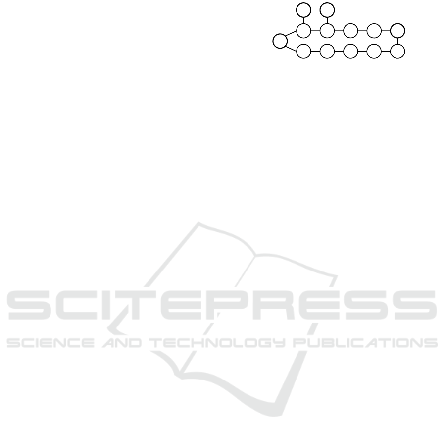
tion. Figure 1 presents a MAPF problem instance

with two agents

and

, with start vertices

and

, and goal vertices

and

, respectively. Here,

the optimal solution minimizing the sum-of-costs

= (s

, E, F, G, H, I, g

)

and

= (s

, B, A, g

)

which yields

SOC

(Π) = 9

and

MKS

(Π) = 6

. The

optimal solution minimizing the makespan is

, A, B,C, D, g

)

and

= (s

, s

, B, A, g

)

, which

𝑔

𝑗

𝑠

𝑗

𝑠

𝑖

𝑔

𝑖

𝑠

𝑗

𝑔

𝑠

𝑔

𝑠

𝐵

𝑔

𝐴

𝑠

𝐷

𝐶

𝑔

𝑠

𝐸 𝐹 𝐺 𝐻 𝐼

Figure 1: Example of a MAPF problem instance with differ-

ent SOC and makespan optimal solutions.

yields

SOC

(Π) = 10

and

MKS

(Π) = 5

. This example

illustrates that both cost functions are indeed different

and optimizing one may increase the other.

3 FINDING OPTIMAL

SOLUTIONS

The basic idea in a reduction-based approach for solv-

ing MAPF is to model agents’ positions in time. The

correct number of timesteps in which the agent may

perform its moves has to be found.

As explained in Section 2, there are two common

cost functions to evaluate the quality of a plan. Finding

makespan optimal solutions is straightforward, as it

follows a basic iterative deepening approach (Surynek

et al., 2016); the makespan is incremented until the

bounded problem becomes satisﬁable. The solution

of the problem at this point is makespan optimal. We

improve this approach by setting a lower bound on the

makespan derived from the shortest paths from start to

goal of each agent. The bound is set to the maximum

of all shortest paths. We refer to increments of this

lower bound as δ.

Finding a sum-of-costs optimal solution is more

involved, as the number of timesteps has to be ﬁgured

out and the sum-of-costs value has to be restricted. Re-

call the example in Figure 1 showing that increasing

makespan (i.e., the number of timesteps) may decrease

the sum-of-costs. There are two main approaches: the

iterative (Surynek et al., 2016) and the jump (Bart

and Svancara, 2019) method. The iterative method

adds a numerical constraint that bounds the sum-of-

costs. Intuitively, this constraint bounds how many

extra actions the agents can perform. Speciﬁcally, the

bound is given by

SOC

(Π

) + δ

, where

is a pos-

sibly conﬂicting plan consisting of shortest paths for

the agents and

is a number of admissible extra moves.

This requires that the number of moves per agent is

bounded by the length of its shortest path plus

. The

number of timesteps in which the agent may move is

set to

+ δ

. With this setup, the iterative method

again follows an iterative deepening approach starting

with a

of zero and increments it until the bounded

problem becomes satisﬁable. The ﬁnal solution is

Improving the Sum-of-Cost Methods for Reduction-Based Multi-Agent Pathﬁnding Solvers

265

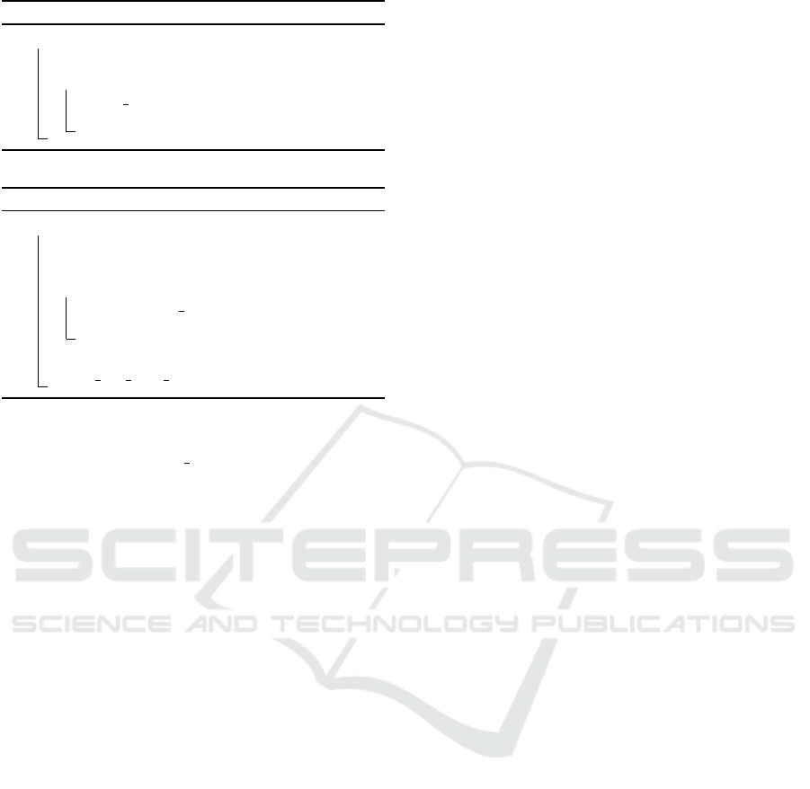
Algorithm 1: Iterative approach.

1 iterative (MAPF problem instance)

2 δ ← 0;

3 while No Solution do

4 solve soc(δ);

5 δ ← δ + 1;

Algorithm 2: Old jump approach.

1 jump-old (MAPF problem instance)

2 δ ← 0;

3 LB(SoC) ← sum of shortest paths;

4 while No Solution do

5 SoC ← solve mks(δ);

6 δ ← δ + 1;

7 δ ← SoC −LB(SoC);

8 solve soc with minimization(δ);

sum-of-costs optimal. Algorithm 1 shows the iterative

approach. Function solve soc takes a MAPF problem

bounded by the given

as described above and solves

it.

The jump method follows a different approach,

as seen in Algorithm 2. First, it starts by ﬁnding a

makespan optimal solution

mks

. We compute the

sum-of-costs

SOC

(Π

mks

)

and use it to ﬁnd an upper

bound on

. Setting

δ = C

SOC

(Π

mks

)−C

SOC

(Π

)

, we

do one last call with the properties explained in the

iterative approach except that the numerical constraint

bounding the total number of moves is replaced by a

minimization component. The number of timesteps is

again set to

+ δ

. Since

is an upper bound, the

minimization component makes sure that the returned

solution is optimal. An important part of this method

is that, when ﬁnding the makespan optimal solution,

we also optimize for the sum-of-costs. This makes

the upper bound on the sum-of-costs tighter. Addi-

tionally, if

SOC

(Π

mks

) = C

SOC

(Π

)

, we have already

found the optimal sum-of-costs solution. Finally, for

a makespan optimal solution

mks

with a

mks

and

SOC

(Π

mks

) = C

SOC

(Π

) + δ

mks

, we have also found

the optimal sum-of-costs solution.

A vital enhancement that applies to the above meth-

ods is what we call reachability, originally introduced

in (Surynek et al., 2016) as MDD graphs. Let

be the

maximum number of moves of an agent

with associ-

ated start and goal vertices

and

, and let

dist(u, v)

be the shortest distance between vertices

and

. We

allow the agent to be at a vertex

at timepoint

only

if the following conditions hold:

dist(s

, v) ≤ t

and

dist(v, g

) + t ≤ t

. That is, if the vertex

can be

reached from the start vertex within

moves and it

is possible to reach the goal vertex from

within the

bound on the maximum moves of the agent. As an

additional enhancement, we block a vertex

for agents

at timepoint

corresponds to the goal vertex of

another

agent and

is larger than the maximum num-

ber of moves of

. This slightly reduces the number of

reachable positions if agents have different bounds on

the number of maximum moves. Note that this block

is implicit in the problem formulation. By adding it to

the reachability deﬁnition we can avoid grounding and

solving effort.

4 ASP ENCODING

We model movements of agents with the encoding

shown in Listing 1. Here, we give an intuitive explana-

tion of the encoding. For a more detailed description

of ASP’s semantics and syntax, we refer to (Gebser

et al., 2015). The encoding assumes as input a MAPF

problem given by the facts, over unary and binary pred-

icates

vertex/1

and

edge/2

, respectively, describing

the graph’s vertices and edges between them. Ad-

ditionally, the facts

agent/1

start/2

, and

goal/2

provide the agents along with their start and goal ver-

tices. The input must include the facts

delta/1

and

dist/2

makespan/1

for sum-of-cost or makespan,

respectively. Predicate

dist/2

captures the length

of the shortest path between each agent’s start and

goal vertices, while

makespan/1

gives the maximum

number of moves each agent can perform. Finally, we

require facts over

reach/3

that encode the reachability

enhancement.

The rules in Lines 1–6 set up the bound on the

maximum number of moves of each agent. For the

sum-of-cost objective, the horizon of the agents is

set individually based on their shortest path and the

given

in Line 2. For the makespan objective, the

horizon of all agents is set to the value given by the

makespan

fact on Line 4. Note that we can selec-

tively ground the programs, so Line 2 is never used

when solving for makespan, while Line 4 is never

used for the sum-of-costs optimization. The choice

rule on Lines 8–9 may choose a move for each agent

conforming to the reachable positions. Observe that

a move to a non-reachable vertex can never happen.

The rule in Line 10 sets the positions of agents at the

ﬁrst timepoint to their starting positions. Line 11 sets

the position of the agent based on the chosen move

while Line 12 keeps the same position if no move was

chosen (wait action). Line 14 ensures that the cho-

sen movement starts at the correct vertex. Line 15

makes sure that the agent is never at a position that

ICAART 2024 - 16th International Conference on Agents and Artiﬁcial Intelligence

266

is not reachable. The rule in Line 16 ensures that

an agent is at exactly one position at every timepoint.

Next, the rules in Lines 18 and 19 encode vertex and

swapping conﬂicts, respectively. Finally, Line 20 en-

sures that an agent is at its goal at the last timepoint.

1 #program su m _of _ cos t s .

2 hor izo n ( A,H +D ) : - dis t ( A,H ), d el ta ( D ).

3 #program ma kes p an .

4 hor izo n ( A,H ) :- ag ent (A ) , ma ke s pan (H).

5 #program mapf .

6 ti me ( A, 1 .. T) :- h or i zo n ( A, T ).

8 {move ( A,U ,V, T ): edge ( U,V ), r ea ch ( A ,V, T ) } 1

9 :- r ea ch ( A,U, T -1).

10 at ( A ,V, 0 ) : - sta rt ( A ,V ), ag en t ( A ) .

11 at ( A ,V, T ) : - m ove ( A,_ ,V, T ).

12 at ( A ,V, T ) : - at ( A, V,T - 1) , no t mo ve ( A ,V , _, T ),

13 ti me ( A, T ) .

14 :- mov e ( A, U,_ ,T ) , no t at ( A,U, T -1).

15 :- at ( A ,V ,T ) , not re ac h ( A, V,T ).

16 :- { at( A,V ,T )} != 1 , tim e ( A,T ).

18 :- { at( A,V ,T )} > 1 , ve rt e x ( V ) , t im e ( _,T ).

19 :- mov e ( _, U,V ,T ) , m ove ( _,V ,U, T ) , U < V .

20 :- goa l ( A,V ), no t at ( A ,V, H ) , hori z on ( A,H ).

Listing 1: ASP encoding for bounded MAPF.

The encoding is sufﬁcient to ﬁnd makespan optimal

solutions. However, for the sum-of-cost objective,

we must add additional rules. We assign penalties to

agents not at their goal position with the following

rules:

pen alt y ( A,N ) :- di st ( A, N + 1) , N >= 0.

pen alt y ( A,T ) :- di st ( A, N ) , at ( A,U ,T ),

not goal ( A,U ) , T >= N .

pen alt y ( A,T ) :- pe n al t y ( A,T +1 ) , T >=0.

The ﬁrst rule applies a penalty to every timepoint

below the shortest path of the agent. At higher time-

points, penalties are applied if agents are not at their

goal positions. Finally, if a penalty was applied at any

timepoint, then every previous timepoint must also

have a penalty. The sum of penalties corresponds to

the cost of a solution.

For the iterative approach, we must also add the

numerical constraint described in Section 3. The fol-

lowing two rules calculate the bound based on the

shortest path of each agent and the given

and enforce

that the sum of costs is below the bound:

bo und (H + D ) : - H=#sum{ T,A : dist ( A,T )} , del ta (D ).

:- #sum{1 ,A, T : pe na l ty ( A,T )} > B, b oun d ( B ).

For the jump approach, we simply minimize the

number of penalties using Clingo’s built-in optimiza-

tion support:

#minimize{1 ,A,T : pe na l ty ( A,T )}.

Algorithm 3: New jump approach.

1 jump (MAPF problem instance)

2 δ ← 0

3 LB(SoC) ← sum of shortest paths

4 while No Solution do

5 SoC ←

solve soc no numerical constraint(

)

6 δ ← inc delta(δ)

7 δ ← SoC −LB(SoC)

8 solve soc with minimization(δ);

5 IMPROVING THE JUMP

APPROACH

In this section, we consider a reﬁnement of the jump

model presented in Section 3. We begin by noting that

the ﬁrst step of ﬁnding a makespan optimal solution is

unnecessarily expensive. Since the main reason to ﬁnd

this initial solution is to get an upper bound on the sum

of costs, any solution works. This leads us to the ﬁrst

and most important enhancement. Instead of ﬁnding

a makespan optimal solution, we use the iterative ap-

proach, disregarding the numerical constraint, to ﬁnd

an initial solution. The reasoning behind this is that the

subproblems that the iterative approach needs to solve

are easier than ﬁnding a makespan optimal solution.

This is because the maximum number of moves of the

agents is bound by the length of their shortest path

and not by the length of the longest shortest path of

all agents. Consequently, the resulting compilation is

smaller and the solving time is reduced. This is com-

bined with the reachability enhancement, where the

reduced movement range of the individual agents leads

to fewer reachable vertices. The potential drawback is

that, due to the reduced movement range of the agents,

it may need a higher

to ﬁnd a solution. However,

since the problems are easier to solve, we expect that

even with the higher number of solver calls, the initial

solution is found much faster.

In the original jump and iterative approaches,

always increased by one to guarantee that the returned

solution is optimal. However, we can overshoot the

bound as we do not need an optimal solution here. This

allows us to increase

in different ways. We introduce

two ways to increase

: a multiplicative increase where

is multiplied by a constant factor, and an additive

increase where δ is increased by a constant value.

The improved jump approach is given in Algo-

rithm 3. Notice that the only differences to the original

jump algorithm are Lines 5 and 6.

Improving the Sum-of-Cost Methods for Reduction-Based Multi-Agent Pathﬁnding Solvers

267

6 BENCHMARKS

We run our experiments on the set of instances stem-

ming from (Hus

ar et al., 2022). The benchmark has

maps with layouts random, room, maze, and empty

and sizes

16 × 16

32 × 32

64 × 64

and

128 × 128

All maps start with 5 agents and the number of agents

increases by 5 up to 100 agents. The instances are also

divided into two categories depending on the length

of the shortest path of the agents. For instances of

type condensed the shortest path length of all agents is

almost the same. Speciﬁcally, for a given instance we

select a length

. The shortest path of the agents is then

within ﬁve percent of

. For instances of type uneven,

the shortest path length of the agents is randomized.

We consider the following functions in Line 6 of

Algorithm 3 to increase the

aside from the basic

increase by one:

• δ ← δ + 2

• δ ← δ + 5

• δ ← δ ∗ 1.5

• δ ← δ ∗ 2

Finally, we compare the default optimization strat-

egy (branch-and-bound) with a strategy based on un-

satisﬁable cores (Andres et al., 2012).

6.1 Results

All benchmarks were run using Clingo 5.6.2 on an

Intel Xeon E5-2650v4 under Debian GNU/Linux 10,

with a timeout of 300 seconds and a memory limit of

28 GB.

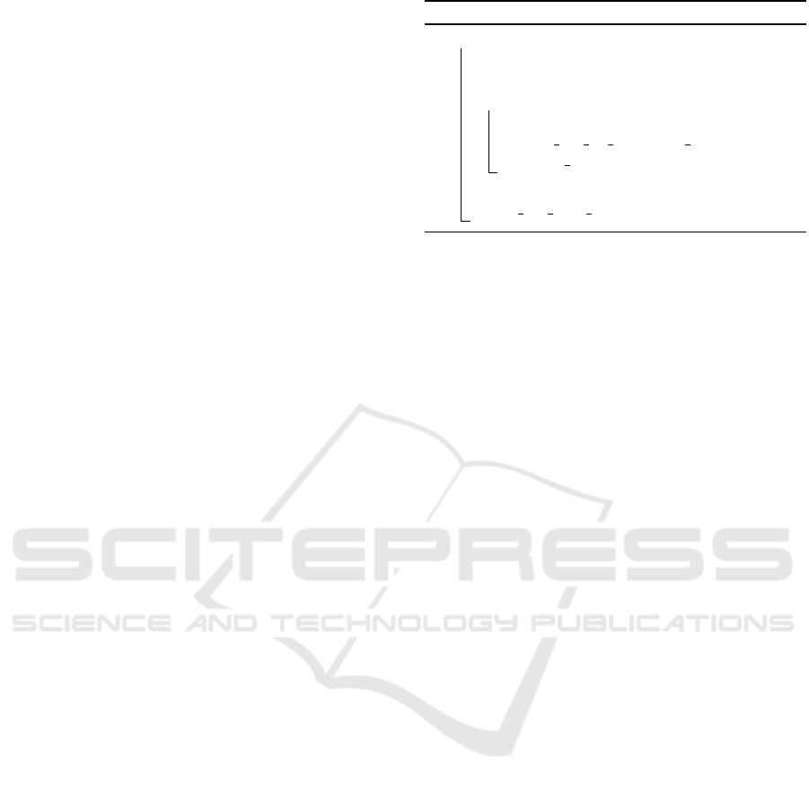
In Table 1, we see the results for the different

increase strategies. The columns report the number of

instances solved for a given size with the total number

of instances in parenthesis. Although all strategies

perform similarly, we see that the increase by two is

the best strategy for the jump approach. Notably, the

increase by ﬁve is the worst strategy. This suggests

that an overly large increase in

is detrimental to

the performance of the jump approach. The bigger

the jump, the bigger the possible overshoot of the

minimum

needed to ﬁnd the ﬁrst solution. This

might lead to a signiﬁcant enough overhead to negate

the advantage of skipping some solver calls. Hence, in

the following discussion, we only include results for

the default increase and the increase by two.

Table 2 shows the total number of instances solved,

separated by size and type. First, we mention that the

chosen optimization strategy has a signiﬁcant impact

on the performance of the jump approach, old and new.

The use of unsatisﬁable cores is signiﬁcantly faster

than the branch-and-bound approach. The approaches

using unsatisﬁable cores managed to solve around 100

more instances than when using branch-and-bound.

For this reason, we only consider the results using

unsatisﬁable cores in the following discussion.

Next, we observe that the jump-old approach is

better than the iterative approach for instances of size

16×16

and

32×32

of type uneven, which is consistent

with the results of (Bart

ak and Svancara, 2019). How-

ever, for the instances of size

64 × 64

and

128 × 128

the performance of the jump-old approach quickly de-

teriorates. This is where the new approach showcases

its strength. We see that it has a similar performance to

the jump-old approach on the smaller instances while

being signiﬁcantly better on the larger instances. Ad-

ditionally, it outperforms the iterative approach on all

instance sizes. We also note that the enhancement

of the jump+2 approach, where

increases by two,

provides a small boost in performance. The other

strategies to increase

similarly provide a small boost

in performance, although, an increase of two seems to

be the best.

Finally, we comment on the instances of type con-

densed. Since all agents have a similar shortest path

length, the reachability calculation is almost the same

regardless of the objective function. Hence, for these

kinds of instances, there is no difference between the

old and new approaches. The results conﬁrm this ob-

servation. The very slight improvement from the new

jump approach is because the condensed instances

have very slight differences in the shortest path length

of the agents.

Table 3 shows the average number of reachable

positions and the average number of calls made to the

solver. We observe how the iterative approach always

has the highest number of calls, followed by jump and

jump-old, in that order. From these numbers, one could

conjecture that the jump-old approach is the best since

it has to solve fewer subproblems. However, looking

at the number of reachable positions, we can see that

although it has to solve fewer subproblems, they are

much more difﬁcult. The trend of the reachable posi-

tions closely resembles the trend of the total number

of instances solved. This is because the number of

reachable positions is a good indicator of the difﬁculty

of the problem. Since the ﬁnal problems that the jump

and jump-old approaches have to solve are likely the

same, the fact that the new approach has an easier time

ﬁnding the ﬁrst solution is the key to its success. We

also note that the results are similar no matter the map

layout.

ICAART 2024 - 16th International Conference on Agents and Artiﬁcial Intelligence

268

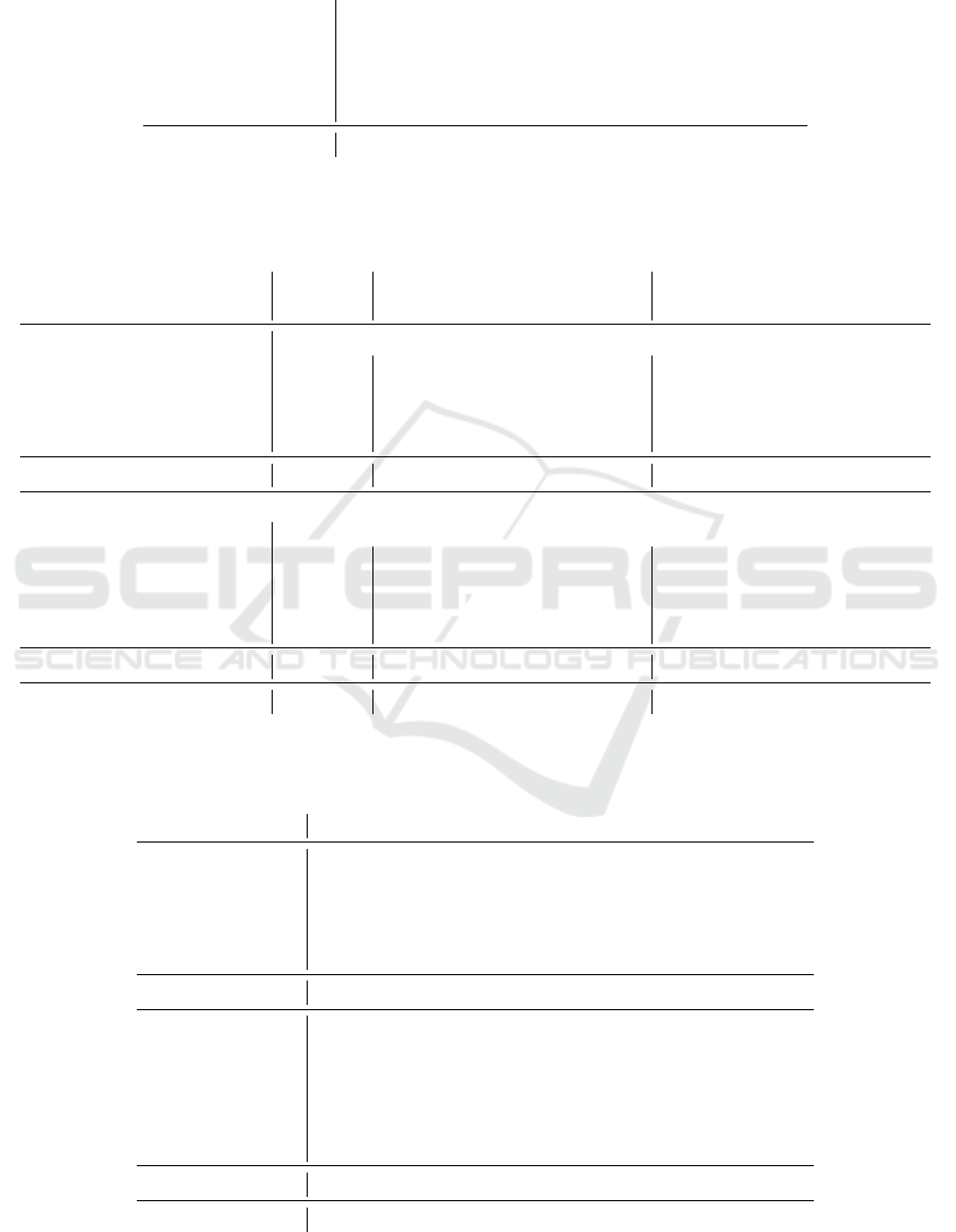
Table 1: Results for all instances grouped by size for the different

increase strategies. The columns report the number of

instances solved with the total number of instances in parenthesis.

jump jump+2 jump+5 jump*1.5 jump*2

16 × 16 (400) 275 275 274 274 273

32 × 32 (400) 371 370 371 372 371

64 × 64 (400)

464 464 462 465 462

128 × 128 (400) 341 346 338 342 342

Total (3200) 1451 1455 1445 1453 1448

Table 2: Results for all instances grouped by size. The columns report the number of instances solved with the total number of

instances in parenthesis.

unsatisﬁable core branch-and-bound

iterative jump-old jump jump+2 jump-old jump jump+2

condensed

16 × 16 (400) 124 137 137 137 127 127 127

32 × 32 (400) 145 161 163 162 144 145 145

64 × 64 (400) 158 184 184 184 159 159 159

128 × 128 (400) 117 137 139 139 122 128 128

Total condensed (1600) 544 619 623 622 552 559 559

uneven

16 × 16 (400) 129 137 138 138 127 127 128

32 × 32 (400) 174 194 208 208 156 190 190

64 × 64 (400) 230 107 280 280 92 247 247

128 × 128 (400) 184 6 202 207 6 194 200

Total uneven (1600) 717 444 828 833 381 758 765

Total (3200) 1261 1063 1451 1455 933 1317 1324

Table 3: Results for all instances solved by all approaches using unsatisﬁable core optimization grouped by size. The columns

report the average cummulative reachable positions in thousands, and the average calls made to the solver in parenthesis.

iterative jump-old jump jump+2

condensed

16 × 16 67 (12.6) 19 (6.2) 19 (6.2) 19 (5.3)

32 × 32 82 (13.4) 23 (6.3) 23 (6.7) 21 (5.5)

64 × 64 122 (11.7) 42 (5.5) 37 (6.5) 37 (5.5)

128 × 128 184 (10.5) 92 (4.0) 76 (6.0) 75 (5.1)

Total condensed 112 (12.1) 42 (5.6) 37 (6.4) 37 (5.4)

uneven

16 × 16 120 (17.4) 44 (3.7) 25 (9.2) 23 (6.7)

32 × 32 175 (11.6) 425 (3.6) 57 (6.6) 52 (5.3)

64 × 64 100 (8.4) 910 (3.4) 40 (5.9) 39 (4.9)

128 × 128 1 (3.0) 270 (3.0) 1 (3.0) 1 (3.0)

Total uneven 137 (12.5) 430 (3.5) 42 (7.2) 39 (5.6)

Total 123 (12.3) 211 (4.7) 39 (6.7) 38 (5.5)

Improving the Sum-of-Cost Methods for Reduction-Based Multi-Agent Pathﬁnding Solvers

269

7 CONCLUSION

While ﬁnding a makespan optimal solution is quite

straightforward, there have been attempts to reﬁne the

algorithm to improve performance (Hus

ar et al., 2022).

The sum-of-cost objective requires more complicated

algorithms as we have bounds on the total cost of the

plan, as well as on the maximum makespan of the

agents. Algorithms to ﬁnd the sum-of-cost optimal so-

lutions for reduction-based solver were ﬁrst conceived

for SAT in (Surynek et al., 2016; Bart

ak and Svancara,

2019). Later, the jump approach was implemented

for ASP in (G

omez et al., 2021), however, the paper

focused mostly on improving the encoding.

In this paper, we have presented a new approach to

ﬁnd a sum-of-cost optimal solution in reduction-based

solvers. The new approach combines the advantages

of both previously known algortihms. It makes use

of the reduced search space of the iterative approach,

while “jumping” to a

that guarantees the existence

of a solution, similarly to the old jump method. Our

experiments show that the new approach is better on

all instance sizes. Additionally, we provide data that

highlights the importance of the optimization strategy

used in the solver. Lastly, we remark that, in practice,

agents usually do not have similar shortest path lengths.

This means the instances of type uneven, where the

best results are seen, are the most realistic.

ACKNOWLEDGEMENTS

This work was partly funded by DFG grant SCHA

550/15, by project 23-05104S of the Czech Science

Foundation, and by CUNI project UNCE 24/SCI/008.

REFERENCES

Andres, B., Kaufmann, B., Matheis, O., and Schaub, T.

(2012). Unsatisﬁability-based optimization in clasp.

In Dovier, A. and Santos Costa, V., editors, Technical

Communications of the Twenty-eighth International

Conference on Logic Programming (ICLP’12), vol-

ume 17, pages 212–221. Leibniz International Proceed-

ings in Informatics (LIPIcs).

Bart

ak, R. and Svancara, J. (2019). On sat-based approaches

for multi-agent path ﬁnding with the sum-of-costs ob-

jective. In Surynek, P. and Yeoh, W., editors, Pro-

ceedings of the Twelfth International Symposium on

Combinatorial Search (SOCS’19), pages 10–17. AAAI

Press.

Bennewitz, M., Burgard, W., and Thrun, S. (2002). Finding

and optimizing solvable priority schemes for decoupled

path planning techniques for teams of mobile robots.

Robotics Auton. Syst., 41(2-3):89–99.

Boyarski, E., Felner, A., Stern, R., Sharon, G., Tolpin, D.,

Betzalel, O., and Shimony, S. (2015). ICBS: Im-

proved conﬂict-based search algorithm for multi-agent

pathﬁnding. In Yang, Q. and Wooldridge, M., editors,

Proceedings of the Twenty-fourth International Joint

Conference on Artiﬁcial Intelligence (IJCAI’15), pages

740–746. AAAI Press.

Dresner, K. M. and Stone, P. (2008). A multiagent approach

to autonomous intersection management. J. Artif. Intell.

Res., 31:591–656.

Gebser, M., Harrison, A., Kaminski, R., Lifschitz, V., and

Schaub, T. (2015). Abstract Gringo. Theory and Prac-

tice of Logic Programming, 15(4-5):449–463.

Gebser, M., Kaminski, R., Kaufmann, B., and Schaub, T.

(2012). Answer Set Solving in Practice. Synthesis Lec-

tures on Artiﬁcial Intelligence and Machine Learning.

Morgan and Claypool Publishers.

omez, R., Hern

andez, C., and Baier, J. (2021). A com-

pact answer set programming encoding of multi-agent

pathﬁnding. IEEE Access, 9:26886–26901.

Hus

ar, M., Svancara, J., Obermeier, P., Bart

ak, R., and

Schaub, T. (2022). Reduction-based solving of multi-

agent pathﬁnding on large maps using graph pruning.

In Faliszewski, P., Mascardi, V., Pelachaud, C., and

Taylor, M., editors, Proceedings of the Twenty-ﬁrst

International Conference on Autonomous Agents and

Multiagent Systems (AAMAS’22), pages 624–632. In-

ternational Foundation for Autonomous Agents and

Multiagent Systems (IFAAMAS).

Kaminski, R., Romero, J., Schaub, T., and Wanko, P. (2023).

How to build your own asp-based system?! Theory

and Practice of Logic Programming, 23(1):299–361.

Kornhauser, D., Miller, G., and Spirakis, P. (1984). Co-

ordinating pebble motion on graphs, the diameter of

permutation groups, and applications. In 25th Annual

Symposium onFoundations of Computer Science, 1984.,

pages 241–250.

Lam, E., Le Bodic, P., Harabor, D. D., and Stuckey, P. J.

(2019). Branch-and-cut-and-price for multi-agent

pathﬁnding. In Proceedings of the Twenty-Eighth In-

ternational Joint Conference on Artiﬁcial Intelligence,

IJCAI-19, pages 1289–1296. International Joint Con-

ferences on Artiﬁcial Intelligence Organization.

Lifschitz, V. (2019). Answer Set Programming. Springer-

Verlag.

Ma, H., Li, J., Kumar, T., and Koenig, S. (2017). Life-

long multi-agent path ﬁnding for online pickup and

delivery tasks. In Proceedings of the Sixteenth Confer-

ence on Autonomous Agents and MultiAgent Systems

(AAMAS’17), pages 837–845. ACM Press.

Sharon, G., Stern, R., Goldenberg, M., and Felner, A. (2011).

The increasing cost tree search for optimal multi-agent

pathﬁnding. In Proceedings of the Twenty-Second In-

ternational Joint Conference on Artiﬁcial Intelligence -

Volume Volume One, IJCAI’11, page 662–667. AAAI

Press.

Stern, R., Sturtevant, N., Felner, A., Koenig, S., Ma, H.,

Walker, T., Li, J., Atzmon, D., Cohen, L., Kumar,

T., Bart

ak, R., and Boyarski, E. (2019). Multi-agent

pathﬁnding: Deﬁnitions, variants, and benchmarks. In

ICAART 2024 - 16th International Conference on Agents and Artiﬁcial Intelligence

270

Surynek, P. and Yeoh, W., editors, Proceedings of the

Twelfth International Symposium on Combinatorial

Search (SOCS’19), pages 151–159. AAAI Press.

Surynek, P. (2010). An optimization variant of multi-robot

path planning is intractable. In Fox, M. and Poole,

D., editors, Proceedings of the Twenty-fourth National

Conference on Artiﬁcial Intelligence (AAAI’10), pages

1261–1263. AAAI Press.

Surynek, P., Felner, A., Stern, R., and Boyarski, E. (2016).

Efﬁcient SAT approach to multi-agent path ﬁnding un-

der the sum of costs objective. In Kaminka, G., Fox,

M., Bouquet, P., H

ullermeier, E., Dignum, V., Dignum,

F., and van Harmelen, F., editors, Proceedings of the

Twenty-second European Conference on Artiﬁcial In-

telligence (ECAI’16), pages 810–818. IOS Press.

Wang, K. C. and Botea, A. (2008). Fast and memory-efﬁcient

multi-agent pathﬁnding. In Proceedings of the Interna-

tional Conference on Automated Planning and Schedul-

ing, ICAPS, pages 380–387.

Yu, J. and LaValle, S. (2013). Structure and intractability of

optimal multi-robot path planning on graphs. Proceed-

ings of the AAAI Conference on Artiﬁcial Intelligence,

27(1):1443–1449.

Improving the Sum-of-Cost Methods for Reduction-Based Multi-Agent Pathﬁnding Solvers

271