ıve Bayes as a Probabilistic Tool for Monitoring the Health Status of

Chronic Patients

Laura Teresa Mart

ınez-Marquina

1 a

, Mar

ıa Teresa Jurado-Camino

1 b

Isabel Caballero-L

opez-Fando

2 c

and Inmaculada Mora-Jim

enez

1 d

Dept. Signal Theory and Communications, Telematics and Computing Systems, Rey Juan Carlos University, Madrid, Spain

University Hospital of Fuenlabrada, Madrid, Spain

Keywords:

Interpretability, Time-Dependent Patterns, Clinical Codes, Sex-Based Model, Clinical Decision Support.

Abstract:

Chronic diseases have emerged as a pervasive global health concern, standing as a leading cause of mortality.

Among these, prevalent conditions encompass diabetes, hypertension, congestive heart failure and chronic

obstructive pulmonary disease. The large amount of data in Electronic Health Records is being exploited by

machine learning schemes to design clinical decision support systems, usually of limited practical application

because of lack of transparency. To overcome this issue and given the dynamic nature of the health-status

over time, we propose here a patient health monitoring scheme based on a N

aive Bayes approach because of

its interpretability, minimal computational cost, and efﬁcient handling of high-dimensional and unbalanced

data. Our approach considers clinical codes (diagnosis and drugs) on real data collected by a Spanish hospital

and provides a probability score for different chronic health-statuses. A gender-based approach has also been

explored, exhibiting promising performance when there is a signiﬁcant patient population for each sex. We

conclude that pharmacological codes are more informative, although the best performance was obtained by

using all the clinical codes and demographic features. Though a more exhaustive study on patient monitoring

is necessary, the proposed NB scheme can be considered a proof of concept which has demonstrated to be a

valuable tool and easily interpretable method.

1 INTRODUCTION

In recent years, there has been an alarming increase in

the number of chronic patients, mainly in developed

countries, due to the aging global population. Nearly

50% of the United States population (Raghupathi and

Raghupathi, 2018) and 35% in Europe (Nolte et al.,

2014), has some type of Chronic Condition (CC). CCs

are the main cause of morbidity, being largely re-

sponsible for activity limitations in older adults and

causing 60% of mortality (Atella et al., 2019). Fur-

thermore, CCs entail signiﬁcant socioeconomic reper-

cussions that directly inﬂuence the healthcare sys-

tem, amounting to 25% of the healthcare budget (Van-

denberghe and Albrecht, 2020). This emphasizes

the need for a paradigm change, drawing the atten-

tion not solely towards treating the illness, but rather

https://orcid.org/0009-0007-4975-1162

https://orcid.org/0000-0002-5646-1290

https://orcid.org/0000-0003-0193-4406

https://orcid.org/0000-0003-0735-367X

towards its prevention (Vandenberghe and Albrecht,

2020) or slowing its progression. In this scenario, ar-

tiﬁcial intelligence and data-driven models can be of

great assistance in achieving the well-known “Triple

Aim” of healthcare systems, which is based on im-

proving patient care experience, enhancing popula-

tion health, and reducing medical care costs (Berwick

et al., 2008).

In the healthcare context, Machine Learning (ML)

is bringing about a true revolution, with increasing

investment in research over the last decade. Auto-

matically deriving insights from longitudinal Elec-

tronic Health Records (EHR) data offers new po-

tential for clinical research, as patient information

evolves through healthcare interactions (Zhao et al.,

2017) across time. One of the main challenges of ML

models on healthcare is their lack of interpretability.

Ignoring this issue could greatly hinder the real-world

utilization of data-driven models (Vellido, 2020).

Owing to the worsening effects of CCs, studying

the temporal progression of chronic patients is vital.

Given that their clinical journey is mirrored in diag-

Martínez-Marquina, L., Jurado-Camino, M., Caballero-López-Fando, I. and Mora-Jiménez, I.

Naïve Bayes as a Probabilistic Tool for Monitoring the Health Status of Chronic Patients.

DOI: 10.5220/0012353000003657

Paper published under CC license (CC BY-NC-ND 4.0)

In Proceedings of the 17th International Joint Conference on Biomedical Engineering Systems and Technologies (BIOSTEC 2024) - Volume 2, pages 393-403

ISBN: 978-989-758-688-0; ISSN: 2184-4305

393

nosis and medication timelines, our paper suggests

utilizing this data for health status monitoring and

prediction. In the clinical setting, these predictions

could be used by healthcare experts to establish in-

tervention measures to slow down the progression of

the CC. Speciﬁcally, in this paper we have considered

demographic and clinical data of chronic patients as-

sociated with the University Hospital of Fuenlabrada

(UHF) in Madrid region (Spain), with the research

being previously approved by the Ethics Committee

of the UHF. Our research group has already pub-

lished some works in this topic, focusing on diabetic

and hypertensive population (Soguero et al., 2020;

Chushig-Muzo et al., 2022; Chushig-Muzo et al.,

2020; Chushig-Muzo et al., 2021). In contrast to our

previous articles, our focus in this paper expands the

variety of CC and delves into the temporal monitor-

ing of the chronic patient’s health status. Speciﬁcally,

we deal here with the following CC: diabetes, hyper-

tension, congestive heart failure, and chronic obstruc-

tive pulmonary disease. Another distinction from our

prior studies involves accounting for the sex variable.

Though both genders demonstrate an escalating CC

risk with age, this rise is often more dramatic among

women (Ellis et al., 2022).

Thus, examining risk factors independently for

men and women could substantially enhance the ef-

ﬁcacy of tailored interventions for each gender.

As in our previous works, the identiﬁcation of

the chronic patients is carried out using the annual

records of each patient and the Clinical Risk Group

population grouper, since it is internationally vali-

dated (Hughes et al., 2004).

To characterize the patient’s health status over

time, we propose in this paper to use the Na

ıve Bayes

(NB) scheme (Mitchell, 1997) due to its simplicity,

efﬁciency in the handling of a large number of vari-

ables, complexity, transparency and interpretability,

all of these very important items in clinical decision

support systems. NB has been successfully applied

within the medical domain (Al et al., 2012; Bhu-

vaneswari and Kalaiselvi, 2012; Hickey, 2013), en-

compassing a wide range of scenarios from estimating

the risk of post-partum depression (Jim

enez-Serrano

et al., 2015) to, more recently, predicting the diagno-

sis of Alzheimer’s disease (Chang et al., 2021). In

this work, the NB approach has been used by con-

sidering both, continuous (age) and categorical vari-

ables (diagnosis and drug codes). As the NB classiﬁer

relies on the Maximum A Posteriori (MAP) decision

rule (Demirbas, 1988), its probabilistic foundation en-

ables identiﬁcation of the most likely CC for a patient

within a speciﬁc time frame, and also its associated

probability. Note that the MAP rule takes into consid-

eration the prior probability for every CC, so a care-

ful analysis when dealing with highly unbalanced CC

must be considered.

The rest of the paper is structured as follows.

Section 2 presents our dataset description and cor-

responding exploratory analysis, focusing on the sex

variable. The methods used for the temporal analysis

and prediction of the patient’s health status are in Sec-

tion 3. Section 4 explains the process followed for the

models’ designs. The results obtained when evalu-

ating different models, just considering demographic

features, their combination with clinical codes, sex-

based models, and the strategy for temporal monitor-

ing are presented in Section 5. Conclusions are drawn

in Section 6.

2 DATASET DESCRIPTION AND

EXPLORATORY ANALYSIS

Demographic and clinical data were extracted from

EHRs linked to the UHF, considering several types

of chronic patients older than 18 years, getting a to-

tal of 16,791 patients (also named samples according

to the ML terminology). Clinical data correspond to

diagnostic and pharmacological records of these pa-

tients, both encoded using internationally recognized

systems. Thus, diagnoses are coded according to the

9th revision of the International Classiﬁcation of Dis-

eases (ICD-9) and pharmaceuticals coded according

to the Anatomical Therapeutic Chemical (ATC) clas-

siﬁcation system (Ronning, 2002).

The ICD-9 code consists of 5 Alpha-Numeric

Characters (ANCs) with a decimal point between

the third and fourth ANCs. Owing to the inclusion

of new codes, this system has been renamed with

the sufﬁx CM (Clinical Modiﬁcations), ultimately re-

ferred to as ICD-9-CM (Association, 2004). The

ATC code consists of 7 ANCs hierarchically struc-

tured into several levels: anatomical (ﬁrst ANC, ﬁrst

letter of the anatomical group where the drug acts),

therapeutic subgroup (second and third ANCs), phar-

macological (fourth ANC), and chemical subgroup

(ﬁfth ANC). Although a quite complete deﬁnition of

the pharmacological code is obtained with the ﬁrst

ﬁve ANCs, the chemical substance (sixth and seventh

ANCs) provides additional information. To reduce

data dimensionality (number of clinical codes) and in

line with the methodology of previous studies in our

group (Chushig-Muzo et al., 2022), we only consider

here the ﬁrst three digits of the ICD-9-CM and the ﬁve

digits of the ATC codes, resulting in 1,517 diagnosis

features and 746 drug features.

As in our previous works (Chushig-Muzo et al.,

HEALTHINF 2024 - 17th International Conference on Health Informatics

394

2022; Soguero et al., 2020; Chushig-Muzo et al.,

2020; Chushig-Muzo et al., 2021), chronic patients

were clinically identiﬁed according to a Population

Classiﬁcation System named Clinical Risk Groups

(CRGs), internationally validated and oriented to-

wards chronic patients (Hughes et al., 2004).

This system considers demographic factors (age

and sex), clinical attributes (diagnoses, procedures,

and medications), and the corresponding dates of pa-

tient encounters over a speciﬁed time frame, typically

one year. Its purpose is to assign each patient to one

of the 1,080 health statuses. The identiﬁcation of the

CRG health groups is denoted by a 5-digit code. The

ﬁrst digit represents the overall patient’s health sta-

tus, with 9 potential core health statutes: 1 (healthy),

2 (signiﬁcant acute disease), 3 (single minor CC), 4

(minor CC in multiple organ systems), 5 (single dom-

inant or moderate CC), 6 (signiﬁcant CCs in multiple

organ systems), 7 (dominant CC in 3 or more organ

systems), 8 (dominant and metastatic malignancies)

and 9 (catastrophic condition). The next three digits

represent a more speciﬁc health condition and are re-

ferred to as base-CRG. The last digit is the severity

level (not considered here).

As CRGs provide a clinically accepted categoriza-

tion for identifying patients with signiﬁcant CCs, they

can be employed as the ground truth to guide a super-

vised ML task and construct a predictive model of the

patient’s health status. For this purpose, this study

considers the more prevalent CCs: Congestive Heart

Failure (CHF), Hypertension (HT), Diabetes (DIA)

and Chronic Obstructive Pulmonary Disease (COPD).

Since we will consider these CC and the combina-

tion of them, ﬁnally we will select only a total of

10 health status groups, from the 1,080 status groups

available in the CRG system. Thus, patients with only

one CC are assigned to CRGs where the ﬁrst digit is

5, i.e, CRG-5179 (CHF), CRG-5192 (HT),and CRG-

5424 (DIA). Note that COPD has not an speciﬁc CRG

group. Individuals with two simultaneous CCs are as-

signed to CRGs starting with the number 6, i.e., CRG-

6190 (CHF and COPD), CRG-6191 (CHF and DIA),

and CRG-6313 (HT and DIA). Groups linked to more

than two simultaneous CCs start with the number 7,

i.e, CRG-7060 (CHF, DIA and COPD), CRG-7080

(CHF, DIA and other CC), CRG-7081 (CHF, COPD

and other CC), and CRG-7140 (HT, DIA and other

CC).

Considering all the previous aspects, the database

comprised 16,791 patients with anonymous data

records from the UHF, each uniquely identiﬁed with

an ID and associated with just one of the aforemen-

tioned 10 CRG groups. For each patient, demo-

graphic data (age, sex) and clinical data (diagnoses,

procedures, drugs) recorded during one year are avail-

able, along with the corresponding registration dates.

All this information is used by the CRG system to

assign every patient to one CRG group. Table 1 sum-

marizes the demographic data per CRG.

Table 1: Statistics per CRG: number of patients, % of

women and age (average, and standard deviation in brack-

ets).

CRG

# Patients Women (in %) Age

5179 114 66.7 68.9(13.8)

5192 10,126 56.3 57.9(12.0)

5424 1,939 40.6 53.9(15.6)

6190 96 56.2 79.0(11.7)

6191 120 66.7 72.6(11.6)

6313 3,228 47.7 62.3(10.7)

7060 159 59.1 70.6(10.9)

7080 93 59.1 73.3(12.5)

7081 187 50.8 80.8(11.9)

7040 729 58.2 67.4(10.9)

Following our previous analysis (Chushig-Muzo

et al., 2022; Soguero et al., 2020; Chushig-Muzo

et al., 2020; Chushig-Muzo et al., 2021), every

patient is characterized by a binary feature vector

x = [x

, x

, ··· , x

, · ·· , x

] with x

∈ {0, 1}, com-

posed by 1,517 diagnoses codes and 746 drug ones

(D = 2,263 features). Each element of x is encoded

with a value of ‘1’ if the corresponding code was reg-

istered for the patient some time during the year, and

with ‘0’ otherwise. Thus, we can compute the pres-

ence rate for each code and CRG, creating the named

“proﬁle” for each CRG when considering all codes in

a bar graph, as shown in other publications (Chushig-

Muzo et al., 2021; Jurado-Camino et al., 2023) and

not presented here for limitation space.

To gain knowledge of the most prevalent clini-

cal code per sex linked to each CRG, an exploration

of the proﬁles was carried out. The presence rate

of the most common diagnosis and pharmacological

codes on each CRG, separated by sex, is summa-

rized in Tables 2 and 3, respectively. Note that the

ICD-9-CM code with the highest presence rate in al-

most all the considered CRGs (excepting CRG-5424)

is ‘401’, representing Essential Hypertension (EHT).

This is a result of the tight relation between HT and

CHF (Pugliese et al., 2020), as well as of the asso-

ciation between insulin resistance and elevated blood

pressure (Sowers, James R and Frohlich, Edward D,

2003). Other diagnosis codes with high rate are ‘428’

(heart failure) and ‘250’ (diabetes mellitus), which are

commonly associated with all CRGs linked to cardio-

vascular and diabetic patients, respectively.

The highest presence rates in pharmacological

Naïve Bayes as a Probabilistic Tool for Monitoring the Health Status of Chronic Patients

395

codes are summarized in Table 3. The most preva-

lent medications start with the letters A, B, C, and

N. In line with the anatomical classiﬁcation previ-

ously presented, these letters represent the Alimen-

tary, Blood, Cardiovascular, and Nervous systems, re-

spectively. Although drugs beginning with A tend

to be more associated with DIA and those beginning

with C with cardiac problems, there are drugs com-

monly used across all CRGs as paracetamol or ibupro-

fen which primarily affect the Nervous system. These

medications show some differences between women

and men, which could be linked with period pains.

Table 2: Presence rate in each CRG when considering six

of the most prevalent ICD-9-CM codes. Highest value for

each CRG and sex (Men M and Women W ) are in bold.

IDC-9-CM Codes

250 272 401 427 428 719

CRG M W M W M W M W M W M W

5179 0.03 0.05 0.29 0.16 0.40 0.42 0.50 0.39 0.67 0.43 0.14 0.14

5192 0.01 0.01 0.18 0.20 0.70 0.68 0.01 0.01 0.00 0.00 0.10 0.16

5424 0.78 0.77 0.17 0.17 0.06 0.07 0.00 0.00 0.00 0.00 0.10 0.12

6190 0.00 0.02 0.47 0.31 0.58 0.66 0.51 0.32 0.79 0.76 0.09 0.12

6191 0.66 0.79 0.24 0.32 0.32 0.63 0.31 0.44 0.48 0.52 0.15 0.17

6313 0.78 0.76 0.22 0.26 0.57 0.63 0.01 0.01 0.00 0.00 0.10 0.16

7060 0.85 0.77 0.42 0.42 0.54 0.58 0.51 0.45 0.66 0.82 0.13 0.12

7080 0.86 0.84 0.57 0.44 0.51 0.65 0.25 0.38 0.62 0.62 0.07 0.11

7081 0.16 0.26 0.23 0.44 0.42 0.59 0.58 0.56 0.85 0.83 0.03 0.10

7140 0.75 0.72 0.24 0.23 0.58 0.62 0.03 0.01 0.01 0.01 0.11 0.15

Table 3: Presence rate in each CRG when considering six of

the most prevalent ATC codes. Highest value for each CRG

and sex (Men M and Women W ) are in bold.

ATC Codes

A02BC A10BA B01AA C03CA C10AA N02BE

CRG M W M W M W M W M W M W

5179 0.69 0.67 0.00 0.00 0.64 0.67 0.76 0.82 0.60 0.46 0.52 0.72

5192 0.33 0.47 0.00 0.00 0.01 0.01 0.02 0.05 0.33 0.35 0.32 0.50

5424 0.27 0.41 0.57 0.49 0.00 0.01 0.01 0.02 0.49 0.44 0.29 0.44

6190 0.97 0.89 0.00 0.00 0.70 0.41 0.92 0.95 0.70 0.44 0.82 0.90

6191 0.74 0.88 0.65 0.38 0.61 0.61 0.95 0.94 0.66 0.72 0.62 0.76

6313 0.42 0.62 0.68 0.68 0.01 0.02 0.05 0.07 0.68 0.69 0.35 0.56

7060 0.91 0.91 0.39 0.37 0.43 0.62 0.97 0.98 0.64 0.62 0.80 0.91

7080 0.80 0.97 0.27 0.42 0.17 0.43 1.00 0.95 0.75 0.58 0.74 0.88

7081 0.96 0.97 0.08 0.10 0.40 0.50 0.99 0.98 0.38 0.47 0.94 0.96

7140 0.65 0.75 0.59 0.62 0.05 0.03 0.12 0.14 0.60 0.66 0.52 0.69

3 METHODS

We present here the fundamentals of the probabilis-

tic approach used for prediction purposes, as well as

the data preprocessing applied for subsequent tempo-

ral monitoring.

3.1 Na

ıve Bayes for Heterogeneous Data

Based on the Bayes’ conditional probability theo-

rem, the NB approach has shown good results un-

der the na

ıve assumption that features are class in-

dependent (Mitchell, 1997). NB belongs to the fam-

ily of MAP classiﬁers (Demirbas, 1988), which cal-

culate the probability of the class conditioned to an

speciﬁc feature vector. It stands out for its strong

computational efﬁciency and ability to handle high-

dimensional data effectively (Hickey, 2013; Al et al.,

2012; Jim

enez-Serrano et al., 2015; Bhuvaneswari

and Kalaiselvi, 2012; Chang et al., 2021). NB can

also use features of diverse nature (heterogeneous

data).

As shown in Equation (1), given a set of C classes

(C = 10 in this work) and vector x, the NB scheme

assigns to x the class maximizing the posterior prob-

ability P(c

|x).

argmax

P(c

|x) = argmax

P(x|c

)P(c

)

P(x)

i = 1, ..., C

(1)

where P(c

) is the prior probability of class c

, P(x|c

)

is the likelihood of class c

and P(x) is the marginal

probability.

For the application of this NB framework, the na-

ture of the considered variables must be taken into

account. In the context of this study, heterogeneous

data are used, considering both binary features (pres-

ence/absence of clinical and pharmacological codes,

represented by features named as x

and coded as

‘1’/‘0’, respectively) and the numerical feature “age”

(represented by the feature named x

). Thus, the

D-dimensional binary vector x is transformed into a

D+1-dimensional one named x’ when considering the

“age” attribute too. As a result, according to NB, the

likelihood of class c

is estimated as:

P(x

′

) =

∏

d=1

P(x

= 1|c

)

(1 −

P(x

= 1|c

))

1−b

P(x

), i = 1, ·· · , C, b ∈ {0, 1}

(2)

with the part within brackets representing the esti-

mation of the likelihood of vector x following the

Bernoulli distribution (Sinharay, 2010), and

P(x

1 |c

) is estimated as the relative frequency of the d-th

feature when it is “on” (x

= 1). However, this may

lead to a probability of 0 for feature values that are

absent in the dataset, signiﬁcantly affecting the esti-

mation provided by Equation (2). To ensure non-zero

likelihoods, a common practice is to apply Laplace

smoothing (Kibriya et al., 2005).

Regarding the “age” variable, since the number of

potential values is high (between 18 and 103 in this

work), to use a frequentist approach with every possi-

ble value can lead to very abrupt changes in the prob-

ability between consecutive age values, especially in

HEALTHINF 2024 - 17th International Conference on Health Informatics

396

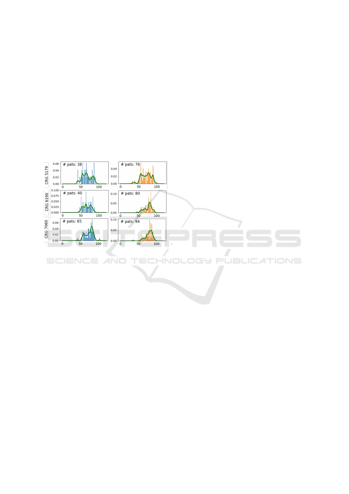
CRGs with few patients. To address this issue, we

proceed as if it were a continuous variable, obtaining

the probability in intervals. In this work, the follow-

ing six intervals were established for x

on the basis

of the exploratory analysis: ≤ 29; 30-40; 41-49; 50-

59; 60-74; ≥75. Though the relative frequency could

be used for estimating probabilities in each interval,

we empirically found using synthetic data that more

acute estimates were provided when getting the prob-

ability density function (pdf ) in a non-parametric way

by using Gaussian kernels and the Parzen windows

method (Parzen, 1962; Silverman, 1986) and then in-

tegrating it to have the corresponding probability. Fig-

ure 1 shows both approaches for CRG-5179, CRG-

6190 and CRG-7060, both for women and men.

Figure 1: Normalized histograms for the age (left panels,

blue, for men; right panels, orange, for women) and corre-

sponding pdf estimation using Parzen windows (in green).

3.2 Data Preprocessing for Temporal

Monitoring

In healthcare, time series are usually irregularly sam-

pled, with irregular temporal intervals between two

consecutive clinical registers. To address this is-

sue,pharmacological data, reported on a monthly ba-

sis, are used in this work. However, the peculiarities

of the Spanish health system, with a different EHR in

each Spanish region (17 regions, with no interoper-

ability between EHRs), can lead to data gaps in one

of them over extended periods of time. These gaps

may arise from factors like lengthy vacation periods,

during which patients are away from their usual res-

idence, resulting in no registration of the medication

dispensation in their region. These gaps manifest as

missing data in the patient’s EHR accessible by the

UHF.

In order to overcome the difﬁculties in the analysis

produced by the lack of encounters with the regional

health system, we carry out a preprocessing stage us-

ing temporal data.

In particular, we propose to use a exponential

weighting function ensuring that the drug presence

is not deactivated abruptly in the next month if the

drug dispensation has not been registered. Instead,

for each feature, exponential weighting functions are

added and the result is used to create the new binary

temporal values for the corresponding feature x

af-

ter thresholding. Figure 2 shows an example of the

temporal vector with twelve months, with the phar-

macy symbol indicating that the drug has been col-

lected (see the binary feature, with ‘1’ value in Feb,

Apr, May, Jul, Oct, Nov and Dec). Since the exponen-

tial function is continuous and we just have one value

per month, the exponential weighting function of one

month length (blue line in Fig. 2) is sampled every

month. As displayed in Figure 2, when the sampled

value is above the threshold (0.5, dotted red line), for

each month the corresponding element is set to ‘1’

(‘0’, otherwise) in the preprocessed feature. The new

temporal sequence of values is shown in Fig. 2 as in-

terpolated monthly feature. Note that, even when the

drug is not dispensed on a monthly basis, the new val-

ues exhibit a scenario most similar to the ideal one

(regular drug dispensation, linked to permanent use

by chronic patients).

To deal with temporal data, it is common the use

of sliding windows (Chen et al., 2017). In this work,

the window length gather data over three months, en-

compassing also data from the preceding two months

before the target month in which we want to predict

the patient’s health status.

4 EXPERIMENTAL DESIGN

We detail here the procedure to create the design and

test sets, to overcome overﬁtting and achieve good

generalization capabilities. Next, the model construc-

tion is explained.

4.1 Experimental Setup

For this study the dataset was split into design and test

sets in a proportion of 70%-30%. The design set, used

to train the NB model using feature vectors summariz-

ing annual encounters, was further split into training

(80%) and validation set (20%). The test set was used

to evaluate the NB model considering two time scales:

annual and quarterly. To avoid a bias linked to the use

of a particular split, 10 different training-validation-

test splits X = {X

, ..., X

} were performed.

Since feature vectors summarize the encounters

over a relatively long period of time (annual or quar-

Naïve Bayes as a Probabilistic Tool for Monitoring the Health Status of Chronic Patients

397

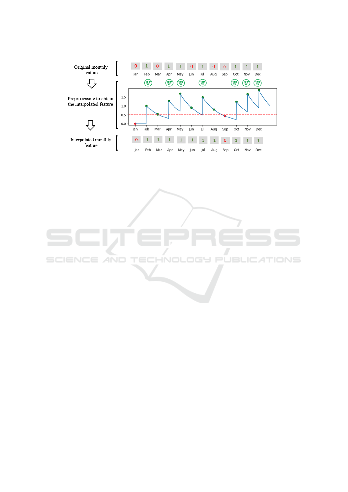
Figure 2: Top panel displays the original monthly feature vector for a speciﬁc drug, with ‘1’ representing the drug dispensation

with a pharmacy symbol in green. Middle panel shows the preprocessing applied to the original feature vector by using an

exponential weighting function (in this case, with 1 month decay, see blue line). Bottom panel represents the preprocessed

feature vector after thresholding the previous blue function with a 0.5 value (dashed red line).

terly), it is possible that different patients are repre-

sented by equal vectors.

Taking this into account, and with the intention of

ensuring an appropriate design, it was checked that

patients assigned to different CRGs were not rep-

resented by the same feature vector. Additionally,

identical vectors associated with the same CRG (448

vectors in total) were temporarily removed from the

dataset and grouped together in the set R . Note that

not all vectors in R are identical among themselves,

but each one has at least another identical feature vec-

tor in R . After the initial split of vectors not included

in R into training, validation and test subsets, similar

vectors in R were proportionally distributed in those

subsets, as shown in Figure 3.

Regarding the sex-based models (separating

women and men), a similar setup was carried out

in parallel, resulting in 10 partitions for women

= {X

, ..., X

} and another 10 for men X

, ..., X

4.2 Na

ıve Bayes Model Construction

and Figures of Merit

Several NB models were explored by using the an-

nual summary of clinical variables. First, two models

using separately diagnoses codes and pharmacologi-

cal codes were considered. Second, a model using

both diagnosis and pharmacological (clinical) data,

together with demographic data, was tackled. Finally,

sex-based models were designed.

The NB performance was assessed using various

ﬁgures of merit. Besides the accuracy rate for each

CRG, we also considered the multiclass Confusion

Matrix (CM) and the multiclass Receiver Operating

Curves, with their corresponding Areas Under the

Curve (AUC) (Hanley and McNeil, 1982). Together

with the AUC per CRG, we also present the Macro-

Average AUC and the Micro-Average AUC (weighted

average based on the number of patients per CRG),

usually used in multiclass tasks (Fodeh et al., 2021).

For each scenario (different input feature vectors),

10 models were designed (one model per partition

in X ). In the case of sex-based models, partitions

and X

were considered. For the NB hyper-

parameter selection, we explored four values of the

Laplace smoothing parameter {0.01, 0.05, 0.1, 0.5},

being 0.05 or 0.1 the most selected values according

to the the Macro-Average AUC on the validation set

(see Figure 3).

5 RESULTS

This section presents the test results using a summary

of the annual data and also considering sex-based

models. The proof of concept with temporal moni-

toring throughout the year, conducted using pharma-

cological data, is ﬁnally presented.

5.1 Using Data Registered over a Year

Binary feature vectors summarizing the patient’s clin-

ical encounters during one year have been considered,

designing two different models: the Diagn-Model

uses only diagnoses features, while the Pharm-Model

just considers pharmacological features. We explored

both equiprobable schemes (yielding best outcomes)

HEALTHINF 2024 - 17th International Conference on Health Informatics

398

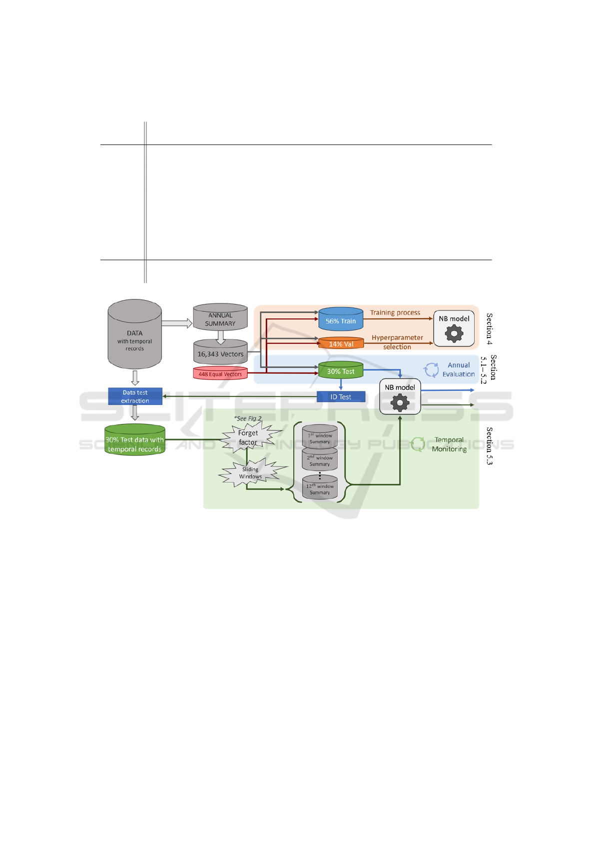
Table 4: Average AUC per CRG (10 test partitions) when using different models, including sex-based ones (rightmost

columns).

CRG

Diagn

Model

Pharm

Model

Clinical&Demog

Model

Clinical&Demog

Men-model

Clinical&Demog

Women-model

5179 0.712 0.801 0.821 0.780 0.840

5192 0.864 0.893 0.952 0.955 0.953

5424 0.793 0.877 0.899 0.903 0.889

6190 0.640 0.711 0.697 0.610 0.636

6191 0.606 0.810 0.775 0.706 0.740

6313 0.729 0.811 0.857 0.869 0.862

7060

0.723 0.734 0.747 0.742 0.752

7080 0.603 0.660 0.636 0.590 0.623

7081 0.800 0.791 0.835 0.829 0.832

7140 0.752 0.725 0.787 0.759 0.803

Macro 0.722 0.782 0.801 0.774 0.793

Micro 0.817 0.862 0.912 0.913 0.914

Figure 3: General framework for the NB model design, annual evaluation and temporal monitoring.

and a priori probability estimates based on the occur-

rence rate. The results presented in this paper corre-

spond to equiprobable schemes.

When analyzing the test CMs with the annual

summary data, we observed that the Diagn-Model

shows more confusion between CRGs linked to one

signiﬁcant CD (CRGs starting with the number 5).

The Pharm-Model, even using a lower number of fea-

tures, improves the results linked to CRGs with dom-

inant CDs in triplets (CRGs starting with the num-

ber 7), which is of paramount interest due to the

worst health status of patients assigned to this kind of

CRGs. These results show that drug codes are more

informative than diagnosis ones.

Analizing the AUC values in Table 4, an improve-

ment in macro and micro AUC is shown when com-

paring the Pharm-Model with the Diagn-model. We

also observe best AUC values for the Pharm-Model

in most of each particular CRG excepting those in the

core health-status number 7 (more than two dominant

CC). This lack of improvement could potentially be

attributed to the lack of speciﬁcity in the third CC

encompassed in this core health-status. Additionally,

note that the annual summary may oversimplify the

patient’s characterization, making the task more difﬁ-

cult due to the complex patients’ health status within

these limited groups.

We also studied the performance when using all

the clinical (diagnosis and pharmacological) codes

and the demographic variable ‘age’. As expected,

the Clinical&Demog-Model provides the best values

of Macro-Average AUC (0.801) and Micro-Average

Naïve Bayes as a Probabilistic Tool for Monitoring the Health Status of Chronic Patients

399

AUC (0.912) and also the highest AUC for most of

the CRGs. Among those showing no improvement

(see Table 4), the CRG-6190 (CHF and COPD) is

often erroneously associated with CRG-7081 accord-

ing to the CMs in Figure 4. This confusion likely

arises due to the shared CCs (CHF and COPD) and

the lack of speciﬁcity in the third CC of CRG-7081

(CHF, COPD, and other CC). Additionally, observa-

tions suggest that when using the Clinical&Demog-

Model, patients within CRG-6191 (CHF and DIA)

display a higher level of confusion with those in CRG-

6313 (HT and DIA). This could be attributed to the

close relationship between CHF and HT, coupled with

the limited speciﬁcity of the diagnosis code linked to

EHT (401, one of the most prevalent codes across sev-

eral CRGs, as shown in Table 2).

5.2 Sex-Based Analysis

The differences found in Section 2 when considering

the “sex” variable suggested us to do a sex-based anal-

ysis when considering the best NB approach. There-

fore, two models using both clinical and demographic

features were created, designed and evaluated with

patients of each sex separately.

Results in Table 4 show that for those CRG

with a large or moderate number of patients (i.e.

CRG-5192, CRG-6313, CRG-5424, with more than

1,000 patients) it is advantageous to design sex-

based models. That is, the AUC provided by any of

the sex-based (women and men) models with more

than 1,000 patients is higher in comparison with the

Clinical&Demog-Model. Apart from that, for CRGs

with a low number of patients and also in compari-

son with the Clinical&Demog-Model, the best AUC is

usually obtained with the sex-based model for which

there is a higher prevalence in the CRG. Thus, this is

the case of CRG-5179 (CHF), CRG-7060 (CHF, DIA

and COPD) and CRG-7140 (HT, DIA and other) for

the women-based model.

5.3 Temporal Monitoring

As previously mentioned in Subsection 3.2, for tem-

poral monitoring it is desirable to work with a series

regularly sampled. Owing to this reason, and also to

the fact that our pharmacological data are automati-

cally registered (they refer to dispensation since are

also used for accounting purposes) and diagnoses are

provided after codiﬁcation of the clinical narrative,

we decided to use the Pharma-Model.

Although chronic patients require a regular intake

of speciﬁc medications, the medication records are

not always consistently recorded on the EHR, and do

not always accurately reﬂect patients’ drug consump-

tion. This can pose a challenge in the application of

ML techniques, reason for introducing the “forget fac-

tor function” which gives exponentially less weight to

the registration of ATC codes as time evolves. Differ-

ent decay rates of the exponential weighting function

were explored, allowing a certain presence of a partic-

ular ATC code to be maintained for more or less time.

Decay values of zero, one, two, and three months

were investigated. In general, as shown in Table 5,

a slower decay of the exponential function led to bet-

ter results in the accuracy rate for each CRG.

The only exception was CRG-5424 (DIA), in

which the lower the decay value, the better the accu-

racy rate. In fact, the best result for this CRG was

achieved with no decay value. This might be due

to the different acute and occasional co-morbidities

associated with diabetic patients, whose occasional

treatment is more reﬂected in the patient’s annual

summary than in the quarterly one.

The accuracy rate obtained with the NB model

trained when considering the presence/absence of

ATC codes during one year are used as a baseline to

evaluate the outcomes of the temporal monitoring (see

ﬁrst row in Table 5).

Regarding the quarterly results, the ﬁrst value of

each cell represents the average accuracy with results

spanning from March to December, encompassing 10

values due to the exclusion of January and February

(as these windows lack three months’ worth of data).

The second value, enclosed in parentheses, indicates

the standard deviation of the accuracy rate. Note that

the average accuracy rate for speciﬁc CRGs (5179,

5424, and 6191) within the quarterly scenario sur-

passes that achieved using annual summary data, par-

ticularly when employing a 3-month decay weight-

ing function. Patients with a more severe health

status, characterized by dominant CCs across three

or more organ systems (indicated by gold-standard

CRGs starting with 7), exhibit a higher accuracy rate

with annual summary data compared to the quarterly

approach. The limited 3-month data collection pe-

riod might not adequately capture all the CC inher-

ent to CRG7, potentially underestimating the patient’s

health condition into other CRGs sharing two of the

CCs.

Continuing with the temporal monitoring, we fo-

cused on analyzing the posterior probabilities esti-

mated by the model within each time window. These

probabilities were examined from two distinct view-

points: (i) First, the posterior probability

P(CRG

|x)

was evaluated in cases where patients were associated

with CRG

; (ii) secondly,

P(CRG

|x) was assessed

for patients not linked to CRG

. In an optimal sce-

HEALTHINF 2024 - 17th International Conference on Health Informatics

400

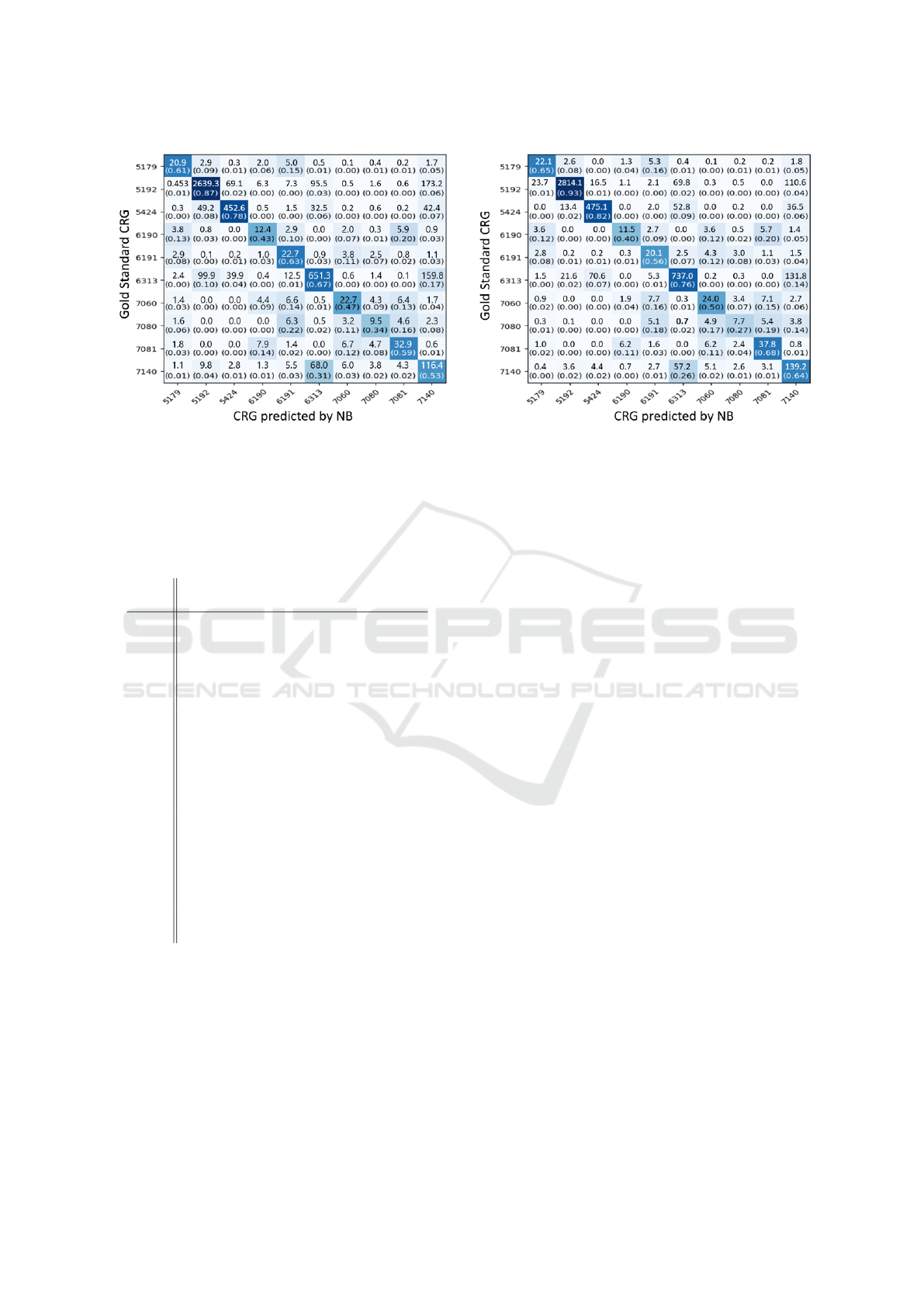
Figure 4: Average CM across the 10 test partitions for both the Pharm-Model (left) and the Clinical&Demog-Model (right).

In each cell: the ﬁrst value indicates the average count of test instances; the number within parentheses is the corresponding

percentage, relative to the CRG established as the gold standard.

Table 5: Accuracy rate for each CRG using the summary

over one year (Ann) and the average rate (and standard de-

viation, in brackets) when using the summary over quarterly

sliding windows (Qua) with different weight decay.

CRG Ann

Qua

0 m.

Qua

1 m.

Qua

2 m.

Qua

3 m.

5179 0.61

0.63

(0.02)

0.65

(0.02)

0.66

(0.01)

0.66

(0.01)

5192 0.87

0.76

(0.01)

0.77

(0.01)

0.78

(0.01)

0.77

(0.01)

5424 0.78

0.88

(0.01)

0.88

(0.01)

0.86

(0.01)

0.85

(0.01)

6190 0.43

0.27

(0.07)

0.33

(0.07)

0.39

(0.02)

0.42

(0.03)

6191 0.63

0.59

(0.02)

0.62

(0.02)

0.64

(0.03)

0.64

(0.03)

6313 0.67

0.60

(0.02)

0.60

(0.02)

0.60

(0.02)

0.60

(0.02)

7060 0.47

0.11

(0.04)

0.15

(0.04)

0.19

(0.04)

0.23

(0.03)

7080 0.34

0.21

(0.03)

0.24

(0.04)

0.28

(0.06)

0.28

(0.07)

7081 0.59

0.15

(0.03)

0.19

(0.03)

0.24

(0.03)

0.28

(0.04)

7040 0.53

0.34

(0.03)

0.38

(0.02)

0.42

(0.03)

0.44

(0.04)

nario, the probabilities in (i) should consistently be

the highest among all those computed for the same

vector x. However, this is not always the case, and

at times, they may not rank as the highest probabili-

ties. As illustrated in Figure 5 for CRG-5179, two box

plots (green and red) were generated for each evalu-

ation. The green boxes represent probabilities when

the NB model correctly assigns the patient to the gold-

standard CRG, while the red boxes depict instances

where

P(CRG-5179|x) isn’t the highest (misclassi-

ﬁed cases). This approach enables an evaluation of

the “conﬁdence” exhibited by the NB model when as-

signing patients to CRG-5179 (in this representation),

while facilitating a comparison of outcomes obtained

from annual and quarterly summary data. Note that,

when considering cases assigned to CRG-5179, the

median of the posterior probabilities (green) consis-

tently remains above 0.8, particularly from the month

of March onward.

Concerning

P(CRG

|x) for patients not associated

with CRG

, the focus is on identifying cases where

this probability holds the highest value, leading to

an incorrect assignment to CRG

. In Figure 6, the

gold standard CRG is presented in the vertical axis

(9 box plots among the 10 CRGs) and probabilities

of the misclassiﬁed samples are organized according

to the actual CRG they are linked to, both for the

annual summary data (left panel) and two represen-

tative situations of the quarterly summary data (two

panels on the right). In this context, a signiﬁcant in-

crease is observed in the number of patients misclas-

siﬁed as CRG-5179, particularly among those orig-

inally linked to CRG-5192, CRG-5424, and CRG-

7140, when quarterly summary data is employed.

However, the probability distribution corresponding

to these misclassiﬁcations remains similar to those es-

timated using annual data.

Naïve Bayes as a Probabilistic Tool for Monitoring the Health Status of Chronic Patients

401

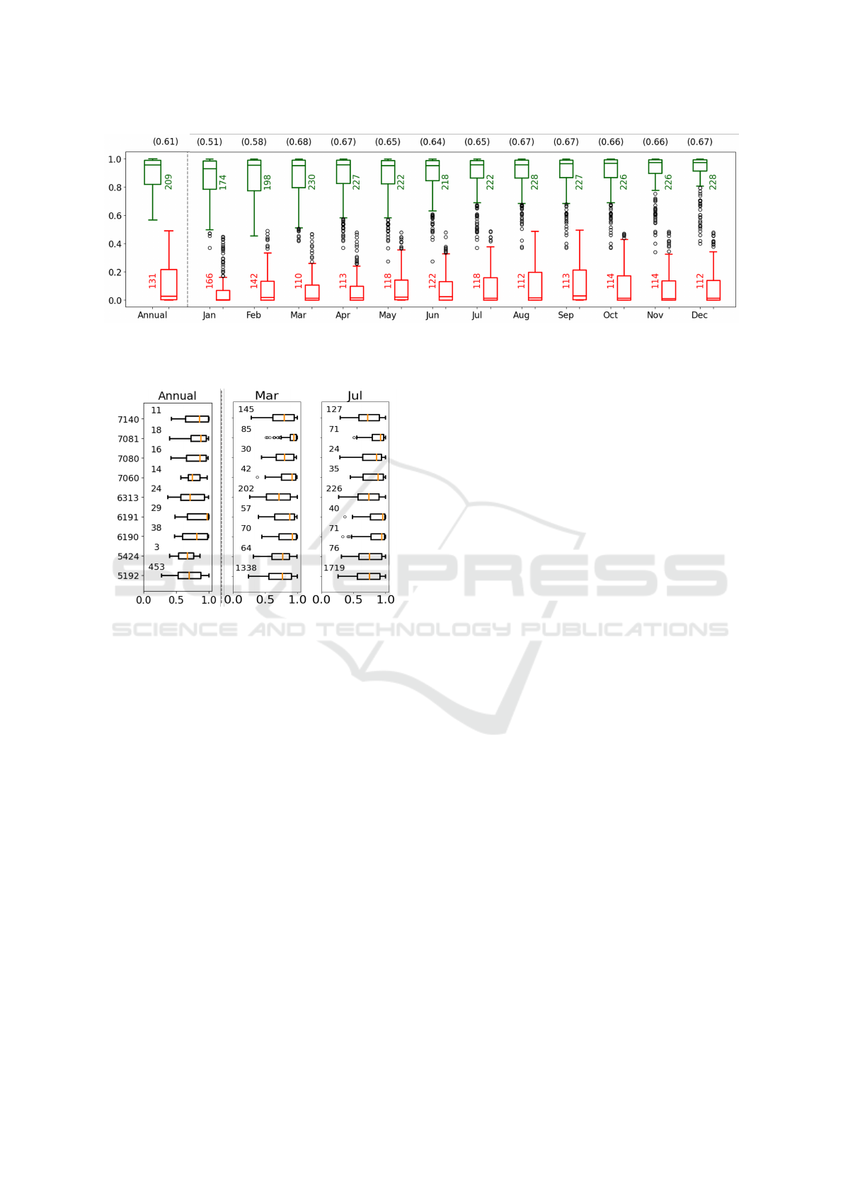
Figure 5: Count of test patients and statistics of

P(CRG−5179|x) for the NB scheme when patients linked to CRG-5179: an-

nual data summary (leftmost panel) and quarterly data summary (3 months) for each month. Green/red, for correctly/wrongly

labelled patients. Accuracy rates are in brackets at the top.

Figure 6: Count of test patients and box plots of

P(GRG−5179|x) when it emerges as the highest value, de-

spite the gold-standard CRG is in the vertical axis. Annual

data (left panel) and quarterly data summary linked to win-

dows centered on March and July (panels right of the dotted

line).

6 CONCLUSIONS AND FUTURE

WORK

Despite the straightforward nature of the Na

ıve Bayes

approach, its application as a tool for identifying and

monitoring patient health statuses has yielded promis-

ing outcomes, particularly when incorporating clini-

cal codes and demographic attributes. Notably, in sce-

narios with a substantial sample size (such as CRG-

5192, 5424, and 6313), an approach based on gen-

der has exhibited advantages. This avenue opens the

opportunity to investigate how gender inﬂuences the

health conditions of chronic patients. Furthermore,

the adoption of a gender-based feature selection strat-

egy could potentially address the issue of high dimen-

sionality, thereby positively impacting the model’s

performance.

Healthcare monitoring involves real data exhibit-

ing a sequential structure, thereby implying that the

interpretation of a pattern can be inﬂuenced by con-

textual information. To take temporal dependencies

into account, we are currently exploring the use of re-

current neuronal models and its application to stream-

ing data, seeking to enhance our monitoring capabili-

ties.

In scenarios involving chronic patients, it would

be also interesting to consider the incorporation of

additional rules within the monitoring framework to

enhance performance. This may be particularly perti-

nent given that the intrinsic nature of CCs indicates

that the patient’s health status (in the context dis-

cussed in this study, denoting CRG assignment) can-

not experience improvement.

ACKNOWLEDGMENT

This work was partly funded by the Spanish Re-

search Agency, grant number PID2019-106623RB-

C41/AEI/10.13039/501100011033 (BigTheory),

PID2022-136887NB-I00 (POLIGRAPH) and by the

European Union NextGeneration-EU funds (Youth

Employment Plan of the Spanish Government) in the

INVESTIGO project with reference URJC-AI-11.

REFERENCES

Al, K. et al. (2012). Medical data classiﬁcation with naive

bayes approach. Information Technology Journal,

11(9):1166–1174.

Association, A. M. (2004). ICD-9-CM 2005: International

Classiﬁcation of Diseases, 9th Revision Clinical Mod-

iﬁcation (Physician Edition). American Medical As-

sociation Press.

Atella, V. et al. (2019). Trends in age-related disease burden

and healthcare utilization. Aging Cell, 18(1):e12861.

HEALTHINF 2024 - 17th International Conference on Health Informatics

402

Berwick, D. M., Nolan, T. W., and Whittington, J. (2008).

The triple aim: care, health, and cost. Health Affairs,

27(3):759–769.

Bhuvaneswari, R. and Kalaiselvi, K. (2012). Naive

bayesian classiﬁcation approach in healthcare appli-

cations. International Journal of Computer Science

and Telecommunications, 3(1):106–112.

Chang, C.-H., Lin, C.-H., and Lane, H.-Y. (2021). Ma-

chine learning and novel biomarkers for the diagnosis

of alzheimer’s disease. Intl. J. Mol. Sci., 22(5):2761.

Chen, M. et al. (2017). Disease prediction by machine

learning over big data from healthcare communities.

IEEE Access, 5:8869–79.

Chushig-Muzo, D., Soguero-Ruiz, C., de Miguel, P., and

Mora-Jim

enez, I. (2021). Interpreting clinical latent

representations using autoencoders and probabilistic

models. Artif Intellig in Medicine, 122:102211.

Chushig-Muzo, D., Soguero-Ruiz, C., de Miguel, P., and

Mora-Jim

enez, I. (2022). Learning and visualizing

chronic latent representations using electronic health

records. BioData Mining, 15(1):1–27.

Chushig-Muzo, D., Soguero-Ruiz, C., Engelbrecht, A.,

de Miguel, P., and Mora-Jim

enez, I. (2020). Data-

driven visual characterization of patient health-status

using electronic health records and self-organizing

maps. IEEE Access, 8:137019–31.

Demirbas, K. (1988). Maximum a posteriori approach

to object recognition with distributed sensors. IEEE

Transactions on Aerospace and Electronic Systems,

24(3):309–313.

Ellis, R. et al. (2022). Development and assessment of a

new framework for disease surveillance, prediction,

and risk adjustment:the diagnostic items classiﬁcation

system. In J Am Med Ass Health Forum, volume 3.

Fodeh, S. J. et al. (2021). Utilizing a multi-class classiﬁ-

cation approach to detect therapeutic and recreational

misuse of opioids on twitter. Computers in Biology

and Medicine, 129:104132.

Hanley, J. A. and McNeil, B. J. (1982). The meaning and

use of the area under a Receiver Operating Character-

istic curve. Radiology, 143(1):29–36.

Hickey, S. J. (2013). Naive bayes classiﬁcation of public

health data with greedy feature selection. Communi-

cations of the Institute of Mathematics and its Appli-

cations, 13(2):7.

Hughes, J. S., Averill, R. F., et al. (2004). Clinical risk

groups (crgs): a classiﬁcation system for risk-adjusted

capitation-based payment and health care manage-

ment. Medical Care, pages 81–90.

Jim

enez-Serrano, S. et al. (2015). A mobile health

application to predict postpartum depression based

on machine learning. Telemedicine and e-Health,

21(7):567–574.

Jurado-Camino, M., Chushig, D., Soguero, C., de Miguel,

P., and Mora, I. (2023). On the use of generative

adversarial networks to predict health status among

chronic patients. In Health Informatics, pages 167–

178.

Kibriya, A. M. et al. (2005). Multinomial naive bayes for

text categorization revisited. In Austr J Conf on Arti-

ﬁcial Intelligence, pages 488–99.

Mitchell, T. M. (1997). Machine Learning. McGraw Hill.

Nolte, E. et al. (2014). Assessing chronic disease man-

agement in european health systems. concepts and ap-

proaches. World Health Organiz.

Parzen, E. (1962). On estimation of a probability den-

sity function and model. The Annals of Mathematical

Statistics, 33(3):1065–76.

Pugliese, N. R. et al. (2020). The renin-angiotensin-

aldosterone system: a crossroad from arterial hyper-

tension to heart failure. Heart Failure Reviews, 25:31–

42.

Raghupathi, W. and Raghupathi, V. (2018). An empirical

study of chronic diseases in the united states: a visual

analytics approach to public health. Intl J. of Env. Re-

search and Public Health, 15(3):431.

Ronning, M. (2002). A historical overview of the atc/ddd

methodology. World Health Organization drug infor-

mation, 16(3):233.

Silverman, B. W. (1986). Density Estimation for Statistics

and Data Analysis. London: Chapman & Hall.

Sinharay, S. (2010). International Encyclopedia of Educa-

tion, chapter Discrete probability distributions. Else-

vier Science.

Soguero, C., Mora, I., Mohedano, M. A., Rubio, M.,

de Miguel, P., and Sanchez, A. (2020). Visually

guided classiﬁcation trees for analyzing chronic pa-

tients. BioMed Central Bioinformatics, 21:1–19.

Sowers, James R and Frohlich, Edward D (2003). Insulin

and insulin resistance: impact on blood pressure and

cardiovascular disease. The Medical clinics of North

America, 87(5):s1005–s1027.

Vandenberghe, D. and Albrecht, J. (2020). The ﬁnancial

burden of non-communicable diseases in the european

union: a systematic review. European Journal of Pub-

lic Health, 30(4):833–839.

Vellido, A. (2020). The importance of interpretability and

visualization in machine learning for applications in

medicine and health care. Neural Computing and Ap-

plications, 32(24):18069–18083.

Zhao, J. et al. (2017). Learning from heterogeneous tem-

poral data in electronic health records. J. Biomedical

Informatics, 65:105–119.

Naïve Bayes as a Probabilistic Tool for Monitoring the Health Status of Chronic Patients

403

REFERENCES

Al, K. et al. (2012). Medical data classification with naive