Fundamental Limitations of Inverse Projections and Decision Maps

Yu Wang

and Alexandru Telea

Department of Information and Computing Science, Utrecht University, 3584 CS Utrecht, The Netherlands

Keywords:

Dimensionality Reduction, Inverse Projections, Decision Maps, Intrinsic Dimensionality.

Abstract:

Inverse projection techniques and decision maps are recent tools proposed to depict the behavior of a classiﬁer

using 2D visualizations. However, which parts of the large, high-dimensional, space such techniques actually

visualize, is still unknown. A recent result hinted at the fact that such techniques only depict a two-dimensional

manifold from the entire data space. In this paper, we investigate the behavior of inverse projections and

decision maps in high dimensions with the help of intrinsic dimensionality estimation methods. We ﬁnd that the

inverse projections are always surface-like no matter what decision map method is used and no matter how high

the data dimensionality is, i.e., the intrinsic dimensionality of inverse projections is always two. Thus, decision

boundaries displayed by decision maps are the intersection of the backprojected surface and the actual decision

surfaces. Our ﬁnding reveals a fundamental problem of all existing decision map techniques in constructing an

effective visualization of the decision space. Based on our ﬁndings, we propose solutions for future work in

decision maps to address this problem.

1 INTRODUCTION

Visualization of high-dimensional data is one of the

key challenges of information visualization (Munzner,

2014). For this goal, dimensionality reduction (DR)

methods, also called projections, are techniques of

choice. DR methods aim to map high-dimensional

data samples into a low-dimensional space while pre-

serving the so-called data structure. DR methods scale

very well both in the number of samples and num-

ber of dimensions and, as such, have gained a strong

foothold in the arena of visualization techniques for

high-dimensional data.

Inverse projection methods aim to construct the

opposite mapping to the one given by a DR tech-

nique – that is, to map points from a low-dimensional

to a high-dimensional space. Recently, inverse pro-

jections have been used to construct so-called deci-

sion maps (Rodrigues et al., 2019; Schulz et al., 2020;

Oliveira et al., 2022). These are two-dimensional im-

ages which aim to capture, in a dense way, the behavior

of a machine learning (ML) model after training.

While both projections and decision maps help

users understand the behavior of high-dimensional

data, they differ in a crucial respect: Decision maps

aim to depict the behavior of a ML model over the

https://orcid.org/0000-0001-6066-0279

https://orcid.org/0000-0002-1129-4628

entire (or at least a large part of the) high-dimensional

space its data comes from. If certain parts of this space

are not covered by a decision map, the users of the

map will have no idea of how the model behaves in

such areas. To trust a decision map, we thus need

to know (a) which parts of the data space it depicts;

and, if not the entire space is covered, (b) how we

can control the depicted spatial subset so as to obtain

actionable insights. In contrast, (inverse) projections

do not have this problem since they are applied to

a ﬁnite set of points to generate a corresponding set

of points. Simply put, (inverse) projections are used

to visualize sets; decision maps are used to visualize

functions (classiﬁcation models).

A recent study (Wang et al., 2023) touched the

question (a) above for the particular case of a single

ML model used to classify a simple three-dimensional

dataset. Surprisingly, the results showed that decision

maps constructed for this case (by three different meth-

ods) only depict a surface embedded in the data space

(see Fig. 1). The rest of the three-dimensional data

space – that is, points not located on this surface – are

not depicted by the decision maps. We have no infor-

mation on how the studied ML model behaves for such

points, even though the model is likely to be used to

classify such samples.

The simple experiment in (Wang et al., 2023) im-

mediately raises several questions:

Wang, Y. and Telea, A.

Fundamental Limitations of Inverse Projections and Decision Maps.

DOI: 10.5220/0012352300003660

Paper published under CC license (CC BY-NC-ND 4.0)

In Proceedings of the 19th International Joint Conference on Computer Vision, Imaging and Computer Graphics Theory and Applications (VISIGRAPP 2024) - Volume 1: GRAPP, HUCAPP

and IVAPP, pages 571-582

ISBN: 978-989-758-679-8; ISSN: 2184-4321

571

Figure 1: Surfaces created by backprojecting to the data space (3D) the decision maps constructed with three different

techniques of an already trained Logistic Regression classiﬁer for a synthetic 6-blobs dataset, adapted from (Wang et al.,

2023). Each surface is colored to show how the classiﬁer assigns one of the six classes to its points. 3D axes are added to the

background to make the shapes of the aforementioned surfaces easier to discern.

Q1.

Does the observation advanced in (Wang et al.,

2023) still hold for different ML models than the

one used in the above study?

Q2.

What exactly are the boundaries we see in Fig-

ure 1? How do these relate to the actual decision

boundaries in high dimensions?

Q3.

Which subsets of the input space do decision maps

cover when the dimensionality thereof is far larger

than three?

Q4.

Do different decision-map construction methods

provide different answers to the above questions?

In this paper, we report a series of experiments

that aim to answer these questions. We construct de-

cision maps for various datasets and classiﬁers us-

ing the three existing decision-map methods avail-

able in the literature (Rodrigues et al., 2019; Schulz

et al., 2020; Oliveira et al., 2022). Next, we pro-

pose a way to quantify their ability to densely sample

their data spaces based on intrinsic dimension estima-

tion (Bennett, 1969; Camastra, 2003; Campadelli et al.,

2015; Bac et al., 2021). We propose several novel visu-

alizations to analyze and compare the obtained results.

Our ﬁndings show that all decision map methods es-

sentially visualize only a surface embedded in high

dimensions, with the exception of areas located very

close to the training samples, no matter what the data

dimensionality is, and no matter which decision map

method is used.

The structure of this paper is as follows. Sec-

tion 2 introduces the background of this work. Sec-

tion 3 presents the visual evaluation for 3D data. Sec-

tion 4 demonstrates the qualitative evaluation for high-

dimensional data. Section 5 discusses our ﬁndings.

Finally, Section 6 concludes this paper and discusses

future work.

2 BACKGROUND

Notations. We start with the notations used next in

this work. Let x

= (x

,... ,x

)

∈ R

1 ≤ i ≤ n

, be

-dimensional data point or sample. Let

D = {

}

j = 1, 2,. .. ,N

, be a dataset of

samples, i.e., a table

with N rows (samples) and n columns (dimensions).

Classiﬁers. A classiﬁcation model (or classiﬁer) is a

function

f : R

→ C (1)

that maps a sample to a class label in a given label-set

. Classiﬁers

are typically constructed by aiming

to satisfy

f (

) = y

for a so-called training set

{(

)}

with x

∈ D

y ∈ C

. A decision zone of

for class

, is the set of points

{

∈ R

| f (

) = y}

; the

boundaries between such decision zones are called the

decision (hyper)surfaces of f .

Projections. A projection, also known as dimension-

ality reduction operation, is a function

P : R

→ R

, (2)

that maps high dimensional data to a low dimensional

(

q ≪ n

) space. For visualization purposes, one most

typically uses

q = 2

. In this case, the projection of a

dataset

, which we denote as

P(D) = {P(

∈ D}

is a 2D scatterplot. Tens of different projection tech-

niques exist with different abilities to capture data-

space similarities

by corresponding similarities in

the projection space

, computational speed, robust-

ness to noise, out-of-sample ability, and ease of use

and implementation. Extensive surveys cover all these

aspects (Espadoto et al., 2019a; Nonato and Aupetit,

2018; Huang et al., 2019; Sorzano et al., 2014; Engel

et al., 2012).

Inverse Projections. An inverse projection (or unpro-

jection (Espadoto et al., 2021a)) is a function

inv

: R

→ R

, (3)

IVAPP 2024 - 15th International Conference on Information Visualization Theory and Applications

572

which, roughly put, aims to reverse the effects of a

given projection

. In more detail, given a dataset

D ∈ R

and its projection scatterplot

P(D)

, an ideal

inverse projection would yield

inv

(P(

)) =

x for all

∈ D

, or more generally minimize, point-wise, the

difference between

and the so-called backprojec-

tion

′

= P

inv

(P(D))

. Note that

inv

is, in most

cases, not the mathematical inverse of

since projec-

tion functions

may not be injective, thus, they are not

invertible. This is so since

can be non-injective, i.e.,

it can map different data points to the same location

(think e.g., of PCA applied to map a point-set

that densely samples the surface of a 3D sphere to the

2D plane; there will be, for any projection plane PCA

computes, exactly two points projecting at the same

location). Also,

can be non-surjective. Indeed, pro-

jections that do not have the so-called out-of-sample

ability only map a given dataset

D ⊂ R

. How

data points outside

would map to

is not handled

by such techniques. This means that, by deﬁnition,

there will be points in

– more precisely, those not

covered by

P(D)

, which do not have a correspondent

in R

via P.

Inverse projections are used to extrapolate the in-

verse mapping constructed as outlined above to points

outside

P(D)

. This enables many applications such as

shape or image morphing (dos Santos Amorim et al.,

2012), data imputation (Espadoto et al., 2021a), and

constructing classiﬁer decision maps (detailed further

below). In contrast to projections, for which many

algorithms exist, only a handful of inverse projection

techniques have been proposed. iLAMP (dos San-

tos Amorim et al., 2012) uses distance-based interpo-

lation with radial basis functions to reverse a speciﬁc

projection technique, LAMP (Joia et al., 2011), which

also uses the same interpolation. NNinv (Espadoto

et al., 2019b) constructs

inv

by deep learning to map

the points of any given 2D scatterplot

P(D)

, con-

structed by any projection technique

, to correspond-

ing points in

. SSNP (Espadoto et al., 2021b) uses

semi-supervised deep learning to construct both a di-

rect and inverse projection, thereby reﬁning earlier

results based on unsupervised autoencoders for the

same goal (Hinton and Salakhutdinov, 2006).

Computing an inverse projection is a more compli-

cated – and actually ill-posed – task that computing a

direct projection, for several reasons. First, an inverse

projection has to revert the effects of a given direct

projection function

, which can be potentially quite

complicated. In contrast, constructing a direct projec-

tion does not need to consider any such earlier-given

mapping. Secondly, as mentioned above, direct pro-

jections often do not admit a mathematical inverse, so

all we can attempt to do is to compute an approximate

or pseudo-inverse. Thirdly, the key use-case for in-

verse projections is to infer data corresponding to 2D

locations where no sample point was projected by the

direct function

– and thereby generate data points

for which no ground-truth information is known (dos

Santos Amorim et al., 2012; Espadoto et al., 2021a).

The issue here is that, for such points, we have no for-

mal means of assessing when, and by how much, our

constructed

inv

is incorrect – thus no hard criterion

to optimize for. In this sense, inverse projections aim

to generalize the inverse mapping corresponding to a

given direct projection, much like ML algorithms aim

to extrapolate their working outside their training sets,

with the fundamental challenges that this extrapolation

implies. This is further discussed below.

Decision Maps. These techniques aim to construct

a dense visual representation of a given trained ML

model

. Given a 2D image

I = {

}

of 2D pixels p,

covers the range of

P(D)

, a corresponding backpro-

jection

inv

= {P

inv

(

∈ I}

is constructed using an

inverse projection

inv

. Next, the pixels p are colored

to depict the labels

f (P

inv

(

))

inferred by the model

Same-color regions in

thus show the decision zones

; neighbor pixels of different colors show the deci-

sion boundaries of

. Decision maps can be used for a

wide range of tasks in explainable AI, such as under-

standing the shapes of the decision zones created by

a trained model (Espadoto et al., 2019b; Sohns et al.,

2023; Zhou et al., 2023), reasoning about the general-

ization ability of such models for unseen data (Schulz

et al., 2020), studying the agreements of different mod-

els (Espadoto et al., 2021a), and dynamic imputation

of data (Espadoto et al., 2021a).

Given that only a few inverse projection techniques

exist (see above), there are also only a few decision

map algorithms. DBM (Rodrigues et al., 2018) di-

rectly applies the above decision-map construction

method by using UMAP (McInnes et al., 2018) and

NNinv (Espadoto et al., 2019b) for the direct, respec-

tively inverse, projection techniques. Several exten-

sions thereof cover the use of additional direct and in-

verse projections and improve DBM’s noise-resistance

by ﬁltering out poorly projected samples (Rodrigues

et al., 2019). SDBM (Oliveira et al., 2022) leverages

SSNP which, as already explained, provides both di-

rect and inverse projections. SDBM yields higher-

quality, smoother, decision maps than DBM but does

not allow one to freely choose

. Finally, Deep-

View (Schulz et al., 2020) leverages discriminative di-

mensionality reduction (Schulz et al., 2015) to enhance

UMAP (McInnes et al., 2018), which also provides an

inverse projection, to construct very high quality deci-

sion maps.

Fundamental Limitations of Inverse Projections and Decision Maps

573

Most work on decision maps only evaluate their

results qualitatively by visually comparing the results

of different such methods against each other for given

datasets and classiﬁers (Rodrigues et al., 2018; Ro-

drigues et al., 2019; Oliveira et al., 2022; Espadoto

et al., 2019c). Oliveira et al. (Oliveira et al., 2023) stud-

ied the stability of DBM and SDBM in presence of

small perturbations of the visualized model, conclud-

ing that these methods are quite robust to such changes.

More recently, Wang et al. (Wang et al., 2023) pro-

vided the most detailed evaluation of decision maps

we are aware of by combining classical ML perfor-

mance metrics (Schulz et al., 2020) with several novel

visual assessments. Additionally, as stated in Sec. 1,

Wang et al. (Wang et al., 2023) showed that DBM,

SDBM, and DeepView only depict a surface in the

case of visualizing a simple classiﬁer trained on a syn-

thetic 3D dataset (Fig. 1). How this ﬁnding extends to

other classiﬁers and higher dimensions is however not

studied. Our paper aims to ﬁll this gap.

To answer the questions in Sec. 1, we conduct

two studies. First, we extend the evaluation in (Wang

et al., 2023) to use additional classiﬁers and visualize

the actual decision boundaries, but still using a 3D

dataset (Sec. 3), thereby answering Q1-Q2. Next, we

investigate the behavior of inverse projections in higher

dimensions and for different datasets (Sec. 4), thereby

answering Q3. Our joint results answer Q4.

3 VISUAL EVALUATION

3.1 Method

We study the behavior of decision maps using six dif-

ferent classiﬁers: Logistic Regression (Cox, 1958),

Support Vector Machines (Cortes and Vapnik, 1995,

SVM), Random Forests (Breiman, 2001), Neural Net-

works, Decision Trees, and K-Nearest Neighbors

(KNN). All the models are implemented using Scikit-

Learn (Pedregosa et al., 2011) with default parameters,

with the exception of the Neural Network, which is

conﬁgured to have three hidden layers, each containing

256 units. We train the above classiﬁers using the well-

known Iris ﬂower dataset (Fisher, 1988). For each clas-

siﬁer, we construct the backprojected decision-map

image

inv

(see Sec. 2), similar to those shown in Fig. 1.

To directly visualize these, we need to have

n = 3

di-

mensions. As such, we restrict the Iris dataset to its

last three features. For ease of visual interpretation of

the constructed images

inv

, we also restrict the dataset

to its last two classes (thus,

|C| = 2

N = 100

). Note

that these two classes are not fully linearly separable,

which makes our classiﬁcation task more challenging

than the synthetic blob dataset used in Fig. 1.

3.2 Results

Figure 2 shows the actual decision zones and decision

boundaries and the backprojected decision maps for six

classiﬁers and three decision-map techniques (DBM,

SDBM, and DeepView). The actual 2D decision maps

are shown in Fig. 3. These results answer Q1-Q2 and

deepen the ﬁndings from (Wang et al., 2023) shown in

Fig. 1 by (1) more classiﬁers, (2) a more challenging

dataset (modiﬁed Iris), and (3) additional visualization

of the actual decision zones and surfaces.

The top row in Fig. 2 shows the backprojected de-

cision maps for the three decision-map techniques. In

all three cases, we see that the backprojected maps

are surfaces that go through the samples of the two

classes (yellow and purple). We however see also dif-

ferences between the three techniques. The backpro-

jected surfaces of DBM and SDBM are quite smooth

and, as such, cannot get very close to (all) the actual

data points. In contrast, DeepView creates a noisier

surface which ‘connects’ the data points. In other

words: DBM and SDBM depict the classiﬁer’s be-

havior further from the training set (extrapolation),

whereas DeepView shows this behavior close to and

inside this set (interpolation). This insight can directly

help users to choose which technique they want to use

depending on where (in data space) they want to study

a given classiﬁer. Another insight relates to the shapes

of the decision maps for different classiﬁers

. For

DBM and SDBM, the projections

of the data points

do not depend on

– see the scatterplots in Fig. 3. As

such, the shape of the backprojected surface is also

independent on

– see Fig. 2. In contrast, DeepView

uses discriminative dimensionality reduction (Schulz

et al., 2015), so its

depends on

. For different clas-

siﬁers, this means different scatterplots (Fig. 3) and

thus different backprojected surfaces (Fig. 2). While

one can argue that this shows more information on

controlling how DeepView’s decision maps actually

sample the data space as a function of

is unclear.

As such, we believe that (S)DBM’s approach, where

this sampling only depends on the training set, is more

intuitive and stable.

We further study the differences between the back-

projected decision map and the actual behavior of the

classiﬁer

as follows. We densely sample the 3D

data space on a voxel grid of size

150

(to limit com-

putational effort); compute, for each voxel, a color

encoding using

at that point; and draw this color-

coded volume half-transparently (Fig. 2, bottom 6

rows). The yellow, respectively purple, volumes are

IVAPP 2024 - 15th International Conference on Information Visualization Theory and Applications

574

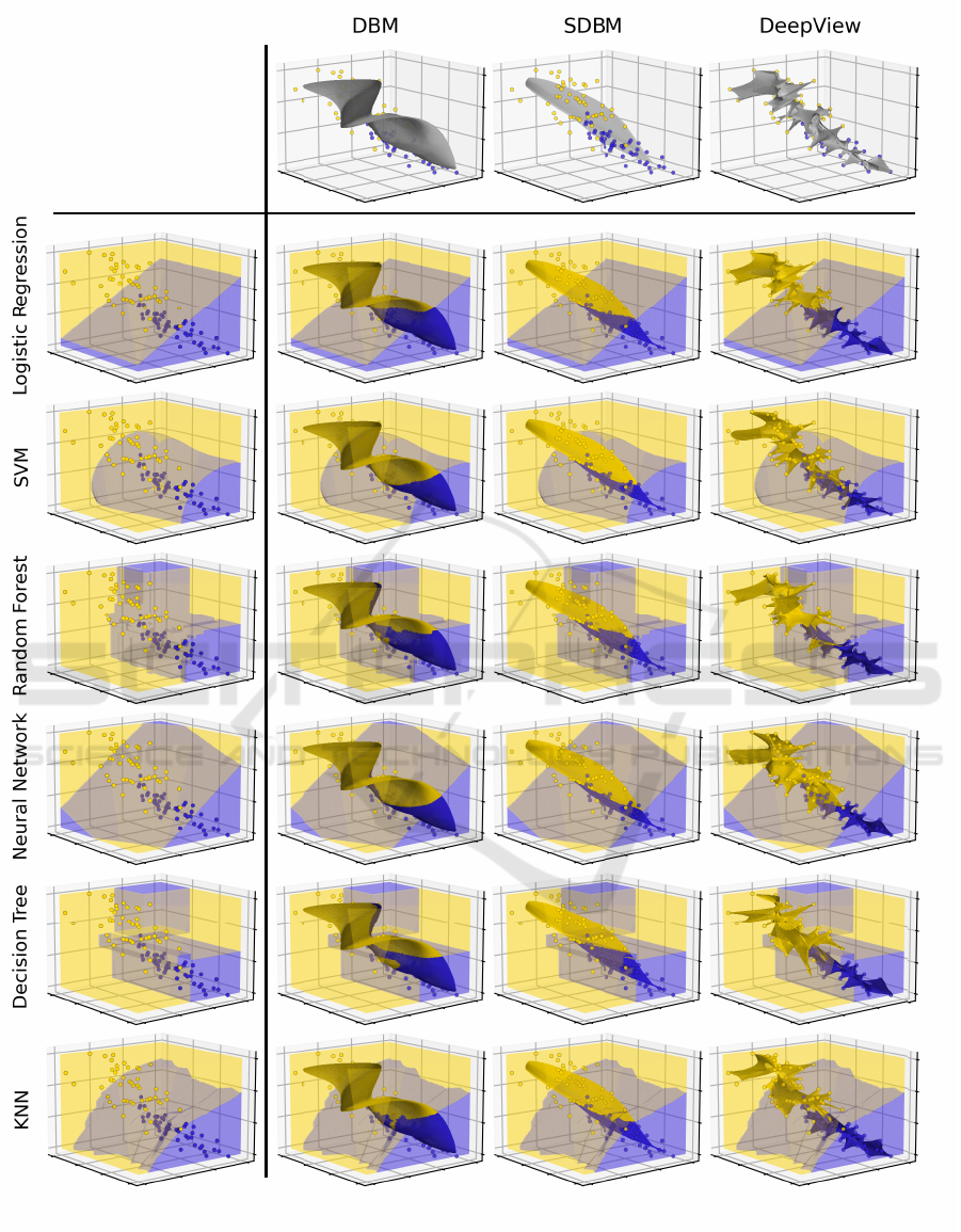
Figure 2: Decision maps of six classiﬁers for the modiﬁed Iris dataset (one row per classiﬁer). The 3D decision zones, i.e., the

ground truth information, are indicated by yellow, respectively purple, with the decision surface separating them in pale brown.

The shaded surfaces embedded in the 3D space show the backprojection of the decision maps constructed by DBM, SDBM,

and DeepView.

Fundamental Limitations of Inverse Projections and Decision Maps

575

DBM SDBM DeepView

Logistic

regression

SVM

Random

forests

Neural

network

Decision

trees

KNN

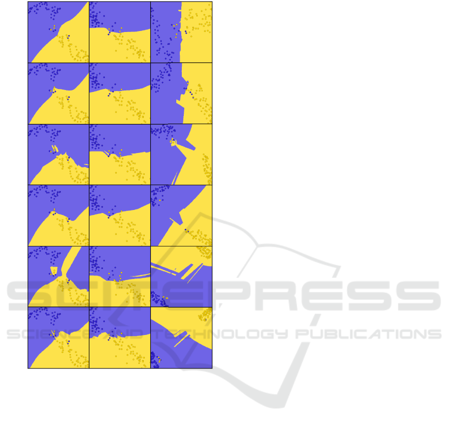
Figure 3: The decision maps corresponding to Fig. 2.

thus the actual decision zones of

. Also, we draw

the actual boundary

that separates the two decision

zones (Fig. 2, bottom 6 rows, pale brown). This is the

actual decision boundary of

. We see that the back-

projected decision map

inv

(shaded surface in Fig. 2),

i.e., the part of the data space that a decision map visu-

alizes, is roughly orthogonal to, and intersecting, the

actual decision surface (pale brown in Fig. 2). That is,

the boundaries which we see in a decision map (curves

where yellow meets purple in Fig. 3) are the intersec-

tion

S ∩ I

inv

. This leads to two important insights: (1)

Decision maps capture global properties of the actual

decision boundaries quite well. For instance, we see

that the actual decision boundaries for SVM, Logistic

Regression, and Neural Networks are quite smooth

as compared to the other three classiﬁers (Fig. 2, left

column). The 2D decision maps also show this insight

(Fig. 3). (2) No decision map technique can actually

claim to visualize the entire decision boundaries of any

classiﬁer. As a consequence, the way these techniques

sample the data space to construct their backprojected

surfaces is very relevant to the insights they produce.

For example, for Decision Trees, we see that the purple

decision zone is actually split into two disconnected

components (top and bottom purple cubes in Fig. 2,

leftmost column). However, only the DBM decision

map shows two separated purple zones (Fig. 3).

4 QUANTITATIVE EVALUATION

4.1 Method

For

n > 3

dimensional data, we cannot directly draw

the backprojected images

inv

. Recall now our ques-

tions Q3 (Sec. 1). To answer it, we measure how

far

inv

is, locally, from a two-dimensional manifold

embedded in

. For this, we use intrinsic dimension-

ality (ID) estimation (Bac et al., 2021) with a linear

ID estimation method, i.e., Principal Component Anal-

ysis (PCA), due to its intuitiveness, computational

efﬁciency, and popularity (Espadoto et al., 2019a; Bac

et al., 2021; Tian et al., 2021), as described next.

Local ID Estimation. Let

be a dataset embedded

. Let

be the

nearest neighbors in

of x

∈ X

Let

λ = (λ

,λ

,. .. ,λ

)

be the

eigenvalues of

’s

covariance matrix, sorted decreasingly, and normalized

to sum up to 1. The ID

is then the smallest

value so that the sum of the ﬁrst

eigenvalues is larger

than a threshold θ (see Alg. 1).

Measurements. We perform two different ID mea-

surements as follows.

First, to study the quality of an inverse projection

inv

, for a given dataset

and its 2D projection

P(D)

we measure the average ID of the backprojection

′

inv

(P(D))

over all neighborhoods

(denoted

′

)

and compare it with the ground-truth average ID of

(denoted

and

′

are computed using

Alg. 1 with

and

′

as inputs, respectively. Ideally,

for a good inverse projection

inv

that reverses well

the effects of the direct projection

, we would obtain

′

= ID

. Secondly, to study how well a decision

map covers the data space it aims to depict, we create

a uniform pixel grid

of size

500

and inverse project

via

inv

to obtain

inv

. We next measure the ID of the

backprojection

inv

at each pixel, denoted by

is computed using Alg. 1 with

inv

as input. We then

visualize

at every location in

and also study its

average value over all pixels in I.

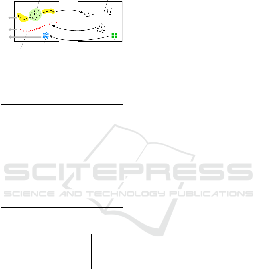
Figure 4 illustrates the process. From the data

points

, we compute a projection

P(D)

. Inversely

projecting these via

inv

yields the backprojection

′

IVAPP 2024 - 15th International Conference on Information Visualization Theory and Applications

576

ℝ

inv

dataset D projection P(D)

pixels Ibackprojection I

inv

backprojection D ’

inv

D’

Figure 4: Computing the intrinsic dimensionality of data,

backprojection of data, and backprojection of pixels.

Inversely projecting a pixel set

yields the backpro-

jection

′

. In this example, the intrinsic dimensionality

is the same to

′

, but higher than

′

, for the

yellow, respective green areas in D.

Algorithm 1: Intrinsic Dimensionality Estimation.

Data: X , set of data points in R

(can be D, D

′

, or I

inv

);

neighborhood size k = 120; threshold θ = 0.95

Result:

d, the estimated ID of X (average among all local

neighborhoods)

1 begin

2 for x

∈ X do

3 Find the k nearest neighbors S of x

in X;

4 Compute the covariance matrix Cov of S;

5 Compute the eigenvalues λ

λ = (λ

,λ

,. .., λ

) of Cov;

6 Sort λ

λ in descending order;

7 Calculate ID d

of S as

= min



∑

j=1

∑

i=1

> θ

8 Calculate average ID

d =

∑

/|X|;

Table 1: Datasets used for ID estimation. For each dataset,

we list the provenance, dimensionality (number of features)

n, number of samples N, and number of classes |C|.

Dataset n N |C|

Blobs 10D (synthetic) 10 5000 10

Blobs 30D (synthetic) 30 5000 10

Blobs 100D (synthetic) 100 5000 10

HAR (Anguita et al., 2012) 561 5000 6

MNIST (LeCun et al., 2010) 784 5000 10

Datasets. We use a mix of synthetic and real-world

datasets, all having

N = 5000

samples (Tab. 1). The

three synthetic datasets consist of

C = 10

isotropic

Gaussian blobs with ambient dimensionality

of 10,

30, and 100. The isotropy of the Gaussian blobs en-

sures that their ID is the same as their dimension count

. For real-world datasets, we use HAR (Anguita et al.,

2012) and MNIST (LeCun et al., 2010). The intrinsic

dimensionality of these datasets has been documented

in prior studies (El Moudden et al., 2016; Facco et al.,

2017; Aum

uller and Ceccarello, 2019; Bahadur and

Paffenroth, 2019), enabling us to juxtapose our ﬁnd-

ings with existing results (see further below). We

further use Logistic Regression as an example classi-

ﬁer. Note that the choice of

does not affect the ID

estimation, as f is not involved in P

inv

’s construction.

Parameter Settings. We set

θ = 0.95

, thereby ac-

counting for 95% of the data variance in

, follow-

ing (Jolliffe, 2002; Fan et al., 2010; Tian et al., 2021).

The size

of the local neighborhood

is another pa-

rameter that needs careful setting. A too large

leads

to overestimating the local ID. A too small

leads to

noisy estimations. Note that

d + 1

independent vectors

are needed to span

dimensions, so

should be at

least equal to the actual ID of

(Verveer and Duin,

1995). For our studied datasets, we have ID ranging

from 13 to 33 for MNIST (Facco et al., 2017; Aum

uller

and Ceccarello, 2019; Bahadur and Paffenroth, 2019);

the ID of HAR ranges from 15 to 61, depending on

the estimation method (El Moudden et al., 2016); our

other synthetic datasets have known ID values ranging

from 10 to 100 (see Tab. 1). As such, we globally set

k = 120 to cover all above cases.

4.2 Results

To answer Q3, we ﬁrst need to see how well an in-

verse projection

inv

covers the data space

it aims to

depict. For this, we compare the estimated ID of the ac-

tual data (

) with that of the round-trip constructed

by direct and inverse projections (

′

). As explained

in Sec. 4.1, ideally

′

= ID

. Table 2 shows our

results for the ﬁve studied datasets. First, we see that

the estimated

aligns well with the ground-truth

values reported for most datasets. As such, we can

compare next the estimated

′

to judge how

good an inverse projection works. The last three rows

of Tab. 2 show a clear result: The inverse projection

always creates a far lower intrinsically-dimensional

dataset than the original one, with DeepView being the

closest (but still far away) from

. This generalizes

our observations for 3D data discussed in Sec. 3.2:

Inverse projections used by (S)DBM create a roughly

two-dimensional, thus surface-like, sampling, of the

high-dimensional data space. In contrast, DeepView

shows a better ability to capture the ID of the data

– which corresponds to our observations showing its

backprojected surfaces having more complex shapes

that aim to connect the data points (Fig. 2).

To further answer Q3, we need to know how well

the pixels of a decision map cover the classiﬁer space

it aims to depict. For this, we measure the ID of the

backprojected decision map image

(see Sec. 4.1)

and compare it with the expected ID of the data. Fig-

ures 5

−

9 show these results for our ﬁve datasets. The

Fundamental Limitations of Inverse Projections and Decision Maps

577

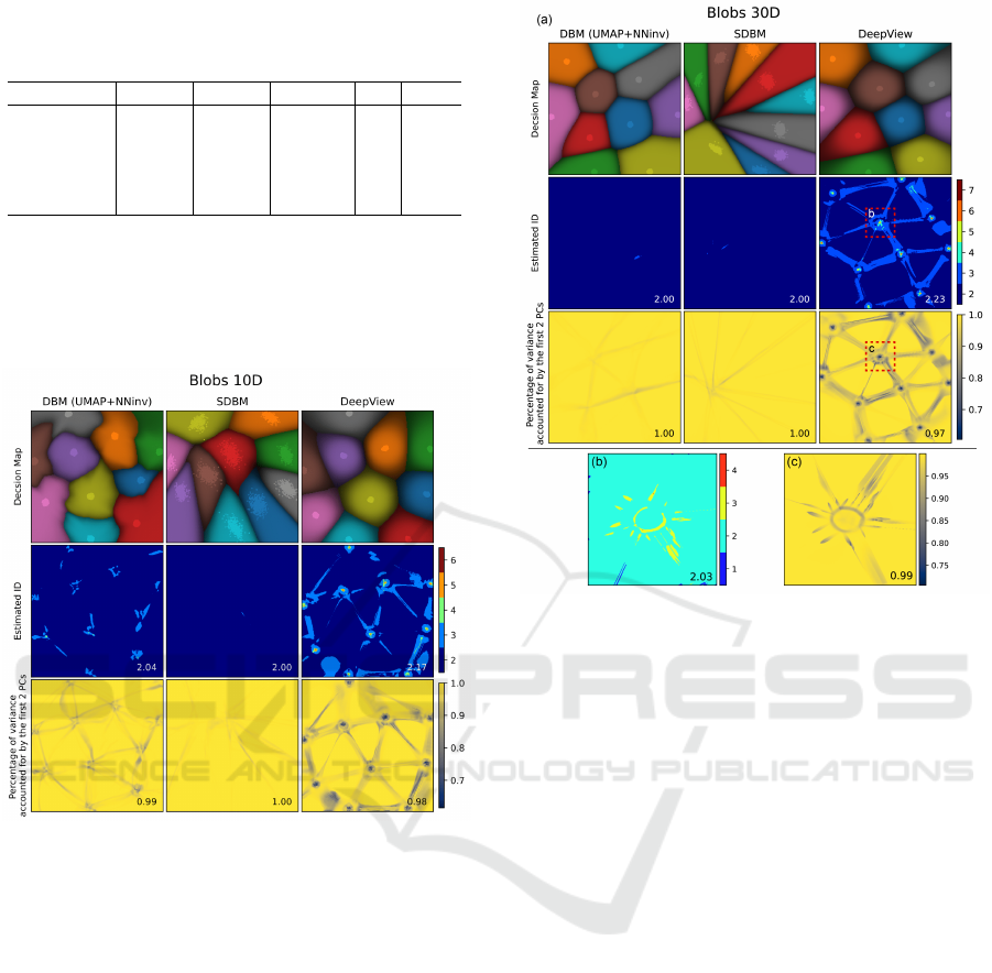
Table 2: Estimated intrinsic dimensionalities

and

′

for our studied datasets. We see that no inverse projection

method can capture the full ID of the data.

Blobs 10D Blobs 30D Blobs 100D HAR MNIST

Expected ID 10 30 100 15-61 13-33

9.67 26.05 66.13 54.01 53.33

′

DBM 2.37 2.00 2.00 2.94 3.85

′

SDBM 2.07 2.00 2.00 2.02 1.96

′

DeepView 3.74 3.58 3.67 6.85 6.02

top rows show the actual decision maps computed by

DBM, SDBM, and DeepView for the studied Logistic

Regression classiﬁer. These images are only provided

for illustration purposes – the subsequent ID analysis

does not depend on the classiﬁer choice.

Figure 5: Decision maps and ID estimation, Blob 10D.

The second rows in Figs. 5−9 show the estimated

for each pixel, with the average

value over

the entire map shown bottom-right in the ﬁgures. Strik-

ingly, the estimated ID for DBM and SDBM are ex-

actly 2 almost everywhere, which means that these

decision maps precisely correspond to surfaces embed-

ded in the high-dimensional space. This generalizes

our earlier observations (Sec. 3.2) to

n > 3

. DeepView

shows a more intricate pattern with higher

values

close to the actual data points (peaking at

= 9

for the HAR dataset); and lower values at map pix-

els far away from the data points (roughly equal to 2

but occasionally dipping to 1 in certain areas of the

MNIST and HAR decision maps). The average

DeepView over all datasets is

2.20 ± 0.03

. To further

understand the higher

values for DeepView, we

select areas having such high values (red squares in

Figs. 6 and 8, second rows). These areas are over-

sampled at a resolution of

500

pixels and

500 × 1000

pixels, respectively. The results (Figs. 6 and 8 (b))

Figure 6: Decision maps and ID estimation, Blob 30D

dataset. Bottom row: Zoom-ins of selected (red) regions.

show that

actually is very close to 2 in such areas

as well. In other words, while DeepView constructs a

more complex-shaped, higher-curvature, surface than

(S)DBM, it still only maps data coming from a surface

in the high-dimensional space.

The third rows in Figs. 5

−

9 reﬁne the above in-

sights by showing the percentage of data variance in

a neighborhood

captured by the eigenvectors cor-

responding to the two largest eigenvalues

and

(computed as in Sec. 4.1). We see that, in most map

regions, this value is close to 1, indicating again that

the decision maps correspond to mostly locally-planar

structures in high-dimensional space. Interestingly,

besides the darker areas corresponding to dense data

points in the projection for DeepView, we see a num-

ber of 1D ﬁlament-like darker structures that span the

image space, for all decision map techniques. These

indicate areas where the backprojected surface

inv

has high curvature. Also interestingly, these ﬁlaments

seem to connect the projected points in DeepView’s

map much like a Delaunay triangulation. This corre-

sponds, for the

n > 3

case, to what we observed earlier

for the

n = 3

case (Fig. 2) – that is, the DeepView

backprojected surface aims to tightly connect the data

samples.

IVAPP 2024 - 15th International Conference on Information Visualization Theory and Applications

578

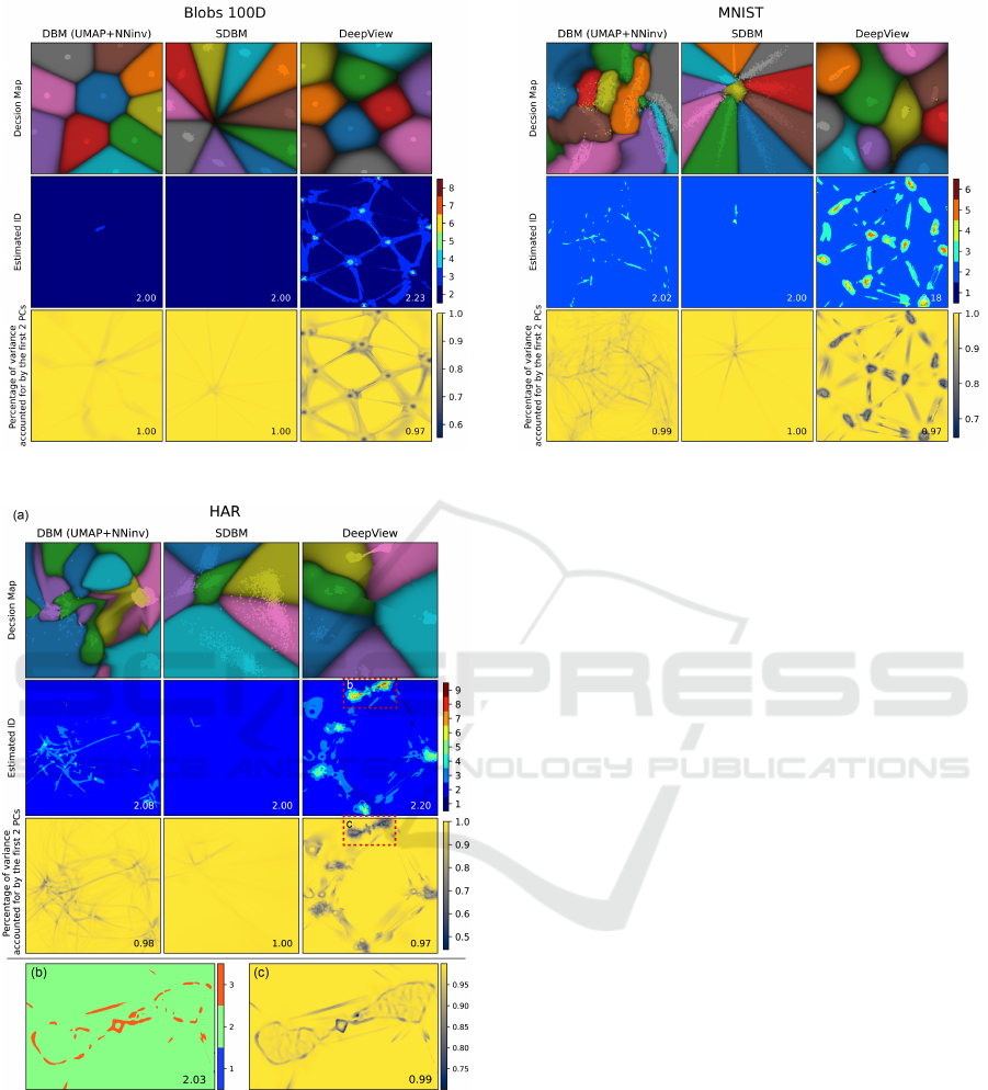
Figure 7: Decision maps and ID estimation, Blob 100D.

Figure 8: Decision maps and ID estimation, HAR. Bottom

row: Zoom-ins of selected (red) regions.

5 DISCUSSION

We next discuss our ﬁndings on the interpretation,

added value, and found limitations of decision maps,

and answer our original questions Q1-Q4.

Surface Behavior of Decision Maps: All three stud-

ied decision map techniques essentially depict surfaces

Figure 9: Decision maps and ID estimation, MNIST.

embedded in the high-dimensional data. This property

does not depend on the intrinsic or total dimensionality

of the studied dataset (Q1) or studied classiﬁer (Q1).

Also, increasing the resolution of the decision map

does not change this aspect (see Figs. 6 and 8). As

such, current decision maps only depict a small part of

the behavior of a given classiﬁer (Q3). The boundaries

that current decision maps show are actually only in-

tersections of these surfaces with the actual decision

boundaries in high-dimensional space (Q2). These are,

we believe, important and previously not highlighted,

limitations of current decision map techniques. We

argue that, without further explanatory tools that as-

sist the user in interpreting decision maps, the insights

given by such maps are limited and can be potentially

even misleading.

One could argue that this surface behavior is ev-

ident from the fact that inverse projections are de-

ﬁned on the 2D image plane and, as such, they will

always construct a surface embedded in higher dimen-

sions. However, this is not necessarily so. Space-

ﬁlling curves, known since long (Peano, 1890), can

map lower-dimensional intervals to completely cover

higher-dimensional ones. Very recent equivalents exist

for space-ﬁlling surfaces (Paulsen, 2023). By compos-

ing such operations, we can imagine dense mappings

between intervals in spaces of any two dimensions

and

q < n

. While it is true that the existing inverse

projection functions we know of (DBM, SDBM, Deep-

View) do arguably not have this fractal-like behavior,

given that they are constructed by composing locally

differentiable mappings, it was not clear – before our

study – how far they are from piecewise-planar map-

pings. This is especially hard to gauge a priori since

Fundamental Limitations of Inverse Projections and Decision Maps

579

these methods use internally complex nonlinear mecha-

nisms such as deep learning. Our study – in particular,

the ID estimation – evaluated precisely this aspect,

with the aforementioned differences highlighted be-

tween these methods. Moreover, our study proposes

a methodology by which new DBM methods – which

may possibly use mappings like the Peano curves men-

tioned above, or any kinds of mappings – can be evalu-

ated to gauge how much of the high-dimensional data

space they actually cover.

Comparing Decision Map Methods. In terms of

the abovementioned surfaces, different decision map

techniques sample the high-dimensional space quite

differently (Q4). As such, they produce different maps

for the same classiﬁer (which, obviously, has a single

ﬁxed set of actual decision surfaces). Each such map

provides unique insights for the same classiﬁer (see

e.g. Fig. 3). While how the decision maps sample the

high-dimensional space depends only on the training

points for (S)DBM, those of DeepView also depend

on the actual classiﬁer. Overall, (S)DBM sample the

classiﬁer along a smoother surface which is farther

away from the training set, whereas DeepView yields

a less smooth surface that aims to connect the training

samples. Both surface types have their advantages and

limitations: Smoother surfaces farther from training

samples are easier to interpret and show better how

a classiﬁer extrapolates from its training set but are

harder to control in terms of where they are actually

constructed; tighter surfaces that connect the training

samples are easier to control in terms of location but

they only interpolate the classiﬁer behavior close to

and between the training points. Importantly, none of

the studied techniques aims to sample a classiﬁer close

to its actual decision boundaries – which, arguably, are

the most interesting areas to understand.

Limitations. Our ﬁndings have several generalization

challenges. First, we only used two real-world datasets.

More such datasets would be needed to strengthen

our observations. A challenge here is to ﬁnd datasets

having well-documented estimations of the intrinsic

dimensionality. Separately, additional methods to es-

timate the intrinsic dimensionality can be used along

our current linear model, e.g., non-linear methods or

methods that automatically adapt the size

of the local

neighborhood to account for varying data densities.

We plan to consider such methods in future work.

6 CONCLUSIONS

We have presented an analysis of the limitations of cur-

rent inverse projection and decision map techniques

used to construct visualizations of the behavior of ma-

chine learning classiﬁcation models. For this, we have

compared the decision zones and boundaries depicted

by three such techniques – DBM, SDBM, and Deep-

View – with the actual zones and boundaries that are

created by six classiﬁers on a three-dimensional real-

world dataset. We found out that the studied maps only

capture a two-dimensional surface embedded in the

data, with different map techniques offering different

trade-offs on how this surface ranges between interpo-

lation and extrapolation of the classiﬁer behavior with

respect to its training set. We further extended our anal-

ysis to high-dimensional data by comparing the intrin-

sic dimensionality of the data with that of the inverse

projection and backprojection of the map to the data

space. We found that all studied map techniques still

only consider locally two-dimensional, thus surface-

like, subsets of the data space for visualization. Fur-

thermore, we showed evidence that the extrapolation

vs interpolation behavior of (S)DBM vs DeepView

generalize also to higher-dimensional data spaces. Our

work highlights fundamental limitations of all studied

decision map techniques in terms of how much of a

classiﬁer’s behavior they capture, but also where and

how they choose to capture this behavior. These limi-

tations are essential to understand when interpreting a

decision map.

We see two possible ways to further overcome the

surface-like limitation of decision maps. First, differ-

ent inverse-projection techniques can be developed to

focus the sampling of the high-dimensional space on

areas where one wants to study a classiﬁer’s behavior

in more detail, e.g., around actual decision boundaries,

rather than on the (less-interesting) areas containing

same-label samples. This is a very complex challenge:

How to design such a sampling method to capture

large, complex, areas of a high-dimensional space

with only a 2D map? An alternative possibility is to

acknowledge that it is impossible to capture all such

areas by a single map. As such, mechanisms can be of-

fered to allow users to interactively specify which data

regions they want to explore. In this direction, Sohns

et al. (Sohns et al., 2023) have proposed an interactive

tool for exploring high-dimensional decision bound-

aries. Yet, this tool only works on local neighborhoods

and uses a linear projection (PCA), which has been

shown to have poor cluster separation (Espadoto et al.,

2019c). Moreover, this technique works only on tabu-

lar data and faces scalability challenges. We believe

that such approaches can be extended by additional in-

teraction mechanisms that allow users to parameterize

the inverse projection to sample speciﬁc regions of the

data space by e.g. controlling the shape and position

of the backprojected surface with respect to the actual

decision boundaries and/or training-set samples.

IVAPP 2024 - 15th International Conference on Information Visualization Theory and Applications

580

REFERENCES

Anguita, D., Ghio, A., Oneto, L., Parra, X., and Reyes-Ortiz,

J. L. (2012). Human activity recognition on smart-

phones using a multiclass hardware-friendly support

vector machine. In Proc. Intl. Workshop on ambient

assisted living, pages 216–223. Springer.

Aum

uller, M. and Ceccarello, M. (2019). The Role of Lo-

cal Intrinsic Dimensionality in Benchmarking Nearest

Neighbor Search. arXiv:1907.07387 [cs].

Bac, J., Mirkes, E. M., Gorban, A. N., Tyukin, I., and

Zinovyev, A. (2021). Scikit-Dimension: A Python

Package for Intrinsic Dimension Estimation. Entropy,

23(10):1368.

Bahadur, N. and Paffenroth, R. (2019). Dimension Esti-

mation Using Autoencoders. arXiv:1909.10702 [cs,

stat].

Bennett, R. (1969). The intrinsic dimensionality of signal

collections. IEEE Trans. Inform. Theory, 15(5):517–

525.

Breiman, L. (2001). Random Forests. Mach. Learn., 45(1):5–

32.

Camastra, F. (2003). Data dimensionality estimation meth-

ods: a survey. Pattern Recognit., 36(12):2945–2954.

Campadelli, P., Casiraghi, E., Ceruti, C., and Rozza, A.

(2015). Intrinsic dimension estimation: Relevant tech-

niques and a benchmark framework. Math. Probl. Eng.,

2015:1–21.

Cortes, C. and Vapnik, V. (1995). Support-vector networks.

Mach. Learn., 20(3):273–297.

Cox, D. R. (1958). Two further applications of a model for

binary regression. Biometrika, 45(3/4):562–565.

dos Santos Amorim, E. P., Brazil, E. V., Daniels, J., Joia,

P., Nonato, L. G., and Sousa, M. C. (2012). iLAMP:

Exploring high-dimensional spacing through backward

multidimensional projection. In Proc. IEEE VAST,

pages 53–62.

El Moudden, I., El Bernoussi, S., and Benyacoub, B. (2016).

Modeling human activity recognition by dimensional-

ity reduction approach. In Proc. IBIMA, pages 1800–

1805.

Engel, D., H

uttenberger, L., and Hamann, B. (2012). A

survey of dimension reduction methods for high-

dimensional data analysis and visualization. In Proc.

IRTG workshop, volume 27, pages 135–149. Schloss

Dagstuhl–Leibniz-Zentrum fuer Informatik.

Espadoto, M., Appleby, G., Suh, A., Cashman, D., Li,

M., Scheidegger, C. E., Anderson, E. W., Chang, R.,

and Telea, A. C. (2021a). UnProjection: Leverag-

ing Inverse-Projections for Visual Analytics of High-

Dimensional Data. IEEE TVCG, pages 1–1.

Espadoto, M., Hirata, N., and Telea, A. (2021b). Self-

supervised Dimensionality Reduction with Neural Net-

works and Pseudo-labeling. In Proc. IVAPP, pages

27–37. SciTePress.

Espadoto, M., Martins, R., Kerren, A., Hirata, N., and Telea,

A. (2019a). Toward a quantitative survey of dimension

reduction techniques. IEEE TVCG, 27(3):2153–2173.

Espadoto, M., Rodrigues, F. C. M., Hirata, N. S. T., and

Hirata Jr, R. (2019b). Deep Learning Inverse Multidi-

mensional Projections. In Proc. EuroVA, page 5.

Espadoto, M., Rodrigues, F. C. M., and Telea, A. (2019c).

Visual analytics of multidimensional projections for

constructing classiﬁer decision boundary maps. In

Proc. IVAPP. SCITEPRESS.

Facco, E., d’Errico, M., Rodriguez, A., and Laio, A. (2017).

Estimating the intrinsic dimension of datasets by a min-

imal neighborhood information. Sci Rep, 7(1):12140.

Fan, M., Gu, N., Qiao, H., and Zhang, B. (2010). Intrinsic

dimension estimation of data by principal component

analysis. arXiv:1002.2050 [cs].

Fisher, R. A. (1988). Iris Plants Database. UCI Machine

Learning Repository.

Hinton, G. E. and Salakhutdinov, R. R. (2006). Reducing the

dimensionality of data with neural networks. Science,

313(5786):504–507.

Huang, X., Wu, L., and Ye, Y. (2019). A review on dimen-

sionality reduction techniques. Int. J. Pattern Recognit.

Artif. Intell., 33(10):1950017.

Joia, P., Coimbra, D., Cuminato, J. A., Paulovich, F. V., and

Nonato, L. G. (2011). Local afﬁne multidimensional

projection. IEEE TVCG, 17(12):2563–2571.

Jolliffe, I. T. (2002). Principal component analysis for spe-

cial types of data. Springer.

LeCun, Y., Cortes, C., and Burges, C.

(2010). MNIST handwritten digit database.

http://yann.lecun.com/exdb/mnist.

McInnes, L., Healy, J., and Melville, J. (2018). UMAP:

Uniform Manifold Approximation and Projection for

Dimension Reduction. arXiv:1802.03426 [cs, stat].

Munzner, T. (2014). Visualization analysis and design. CRC

press.

Nonato, L. and Aupetit, M. (2018). Multidimensional pro-

jection for visual analytics: Linking techniques with

distortions, tasks, and layout enrichment. IEEE TVCG,

25:2650–2673.

Oliveira, A. A. A. M., Espadoto, M., Hirata, R., and Telea,

A. C. (2023). Stability Analysis of Supervised Decision

Boundary Maps. SN COMPUT. SCI., 4(3):226.

Oliveira, A. A. A. M., Espadoto, M., Hirata Jr, R., and

Telea, A. C. (2022). SDBM: Supervised Decision

Boundary Maps for Machine Learning Classiﬁers. In

Proc. IVAPP, pages 77–87.

Paulsen, W. (2023). A Peano-based space-ﬁlling surface of

fractal dimension three. Chaos, Solitons & Fractals,

168.

Peano, G. (1890). Sur une courbe, qui remplit toute une aire

plane. Mathematische Annalen, 36(1):157–160.

Pedregosa, F., Varoquaux, G., Gramfort, A., Michel, V.,

Thirion, B., Grisel, O., Blondel, M., Prettenhofer,

P., Weiss, R., and Dubourg, V. (2011). Scikit-learn:

Machine learning in Python. J. Mach. Learn. Res.,

12:2825–2830.

Rodrigues, F. C. M., Espadoto, M., Hirata, R., and Telea,

A. C. (2019). Constructing and Visualizing High-

Quality Classiﬁer Decision Boundary Maps. Infor-

mation, 10(9):280.

Fundamental Limitations of Inverse Projections and Decision Maps

581

Rodrigues, F. C. M., Hirata, R., and Telea, A. C. (2018).

Image-based visualization of classiﬁer decision bound-

aries. In Proc. SIBGRAPI, pages 353–360. IEEE.

Schulz, A., Gisbrecht, A., and Hammer, B. (2015). Using

discriminative dimensionality reduction to visualize

classiﬁers. Neural Process. Lett., 42:27–54.

Schulz, A., Hinder, F., and Hammer, B. (2020). DeepView:

Visualizing Classiﬁcation Boundaries of Deep Neural

Networks as Scatter Plots Using Discriminative Dimen-

sionality Reduction. In Proc. IJCAI, pages 2305–2311.

Sohns, J.-T., Garth, C., and Leitte, H. (2023). Decision

Boundary Visualization for Counterfactual Reasoning.

Comput. Graph. Forum, 42(1):7–20.

Sorzano, C. O. S., Vargas, J., and Montano, A. P. (2014).

A survey of dimensionality reduction techniques.

arXiv:1403.2877 [stat.ML].

Tian, Z., Zhai, X., van Driel, D., van Steenpaal, G., Espadoto,

M., and Telea, A. (2021). Using multiple attribute-

based explanations of multidimensional projections

to explore high-dimensional data. Comput. Graph.,

98:93–104.

Verveer, P. J. and Duin, R. P. W. (1995). An evaluation

of intrinsic dimensionality estimators. IEEE PAMI,

17(1):81–86.

Wang, Y., Machado, A., and Telea, A. (2023). Quantitative

and Qualitative Comparison of Decision-Map Tech-

niques for Explaining Classiﬁcation Models. Algo-

rithms, 16(9):438.

Zhou, T., Cai, Y., An, M., Zhou, F., Zhi, C., Sun, X., and

Tamer, M. (2023). Visual interpretation of machine

learning: Genetical classiﬁcation of apatite from vari-

ous ore sources. Minerals, 13(4):491.

IVAPP 2024 - 15th International Conference on Information Visualization Theory and Applications

582