Multiple Agents Dispatch via Batch Synchronous Actor Critic in

Autonomous Mobility on Demand Systems

Jiyao Li and Vicki H. Allan

Department of Computer Science, Utah State University, Logan, Utah, U.S.A

Keywords:

Autonomous Mobility on Demand (AMoD) Systems, Vehicle Repositioning, Task Assignment, Multiagent

Reinforcement Learning (MARL).

Abstract:

Autonomous Mobility on Demand (AMoD) systems are a promising area in the emerging ﬁeld of intelligent

transportation systems. In this paper, we focus on the problem of how to dispatch a ﬂeet of autonomous

vehicles (AVs) within a city while balancing supply and demand. We ﬁrst formulate the problem as a Markov

Decision Process (MDP) of which the goal is to maximize the accumulated average reward, then propose the

Multiagent Reinforcement Learning (MARL) framework. The Temporal-Spatial Dispatching Network (TSD-

Net) that combines both policy and value network learns representation features facilitating spatial information

with its temporal signals. The Batch Synchronous Actor Critic (BS-AC) samples experiences from the Rollout

Buffer with replacement and trains parameters of the TSD-Net. Based on the state value from the TSD-Net,

the Priority Destination Sampling Assignment (PDSA) algorithm deﬁnes orders’ priority by their destinations.

Popular destinations are preferred as it is easier for agents to ﬁnd future work in a popular location. Finally,

with the real-world city scale dataset from Chicago, we compare our approach to several competing baselines.

The results show that our method is able to outperform other baseline methods with respect to effectiveness,

scalability, and robustness.

1 INTRODUCTION

As urban populations have increased all over the

world, the transportation scene in most metropolitan

areas had been dominated by an ever-increasing num-

ber of private vehicles (UN, 2015). While highly con-

venient for individuals, a community containing an

excessive number of vehicles may ﬁnd itself experi-

encing numerous social and environmental problems,

including air pollution, parking limitations, high en-

ergy consumption, and trafﬁc congestion. The emer-

gence of Autonomous Mobility on Demand (AMoD)

systems is a promising alternative to the paradigm of

private vehicles. The AMoD systems manage a ﬂeet

of autonomous vehicles (AVs) around a city. Passen-

gers place orders through smart devices such as cell-

phones or tablets, and the AMoD platform dispatches

AVs to provide them with fast, point-to-point travel

services.

Dispatching a ﬂeet of AVs across a city while

maintaining balance between supply (AVs) and de-

mand (orders) is one of the important operations in

AMoD systems. In general, the dispatching operation

comprises two primary tasks: (i) repositioning vacant

AVs to locations where rider requests occur, enabling

them to get closer to potential passengers, and (ii) as-

signing suitable orders to available AVs for delivery

to the required areas through ride-matching.

However, coordinating multiple AVs in a dynamic

environment is extremely difﬁcult: (i) occurrences of

orders are unknown both with respect to time and lo-

cation, and the quantity of orders are constantly ﬂuc-

tuating over space and time; (ii) multiple AVs work-

ing under the same system may affect each other; (iii)

customers may cancel the service when the waiting

period exceeds their patience.

Most previous research work that applied Deep

Reinforcement Learning (DRL) to solve these prob-

lems still suffers from certain limitations: (i) it takes

so long to collect experiences for the AMoD system

that AVs are unable to effectively interact with the en-

vironment in real-time. (ii) most neural network ar-

chitectures of the AMoD system only consider spatial

information from the environment but ignore tempo-

ral properties behind the spatial distribution.

To address the challenges and limitations in

AMoD systems, we propose a Multiagent Reinforce-

ment Learning (MARL) framework. Our contribu-

198

Li, J. and Allan, V.

Multiple Agents Dispatch via Batch Synchronous Actor Critic in Autonomous Mobility on Demand Systems.

DOI: 10.5220/0012351700003636

Paper published under CC license (CC BY-NC-ND 4.0)

In Proceedings of the 16th International Conference on Agents and Artiﬁcial Intelligence (ICAART 2024) - Volume 2, pages 198-209

ISBN: 978-989-758-680-4; ISSN: 2184-433X

tions are:

• We propose a new neural network architecture

named Temporal-Spatial Dispatching Network

(TSD-Net) that combines both policy network

(Actor) and value network (Critic). Also, the

Gated Recurrent Units (GRU) are embedded to

process temporal signals behind spatial informa-

tion.

• To improve the efﬁciency of the training proce-

dure, we designed a Batch Synchronous Actor

Critic (BS-AC) algorithm. Instead of spending

a long time to collecting experiences, the BS-AC

samples experiences with replacement to quickly

achieve effective results.

• To address the issue of insufﬁcient supply during

peak hours, we employ the Priority Destination

Sampling Assignment (PDSA) algorithm. This

algorithm is utilized to select the riders with the

most preferred destinations when supply is insuf-

ﬁcient to satisfy all riders.

• To verify the effectiveness, scalability and robust-

ness of our framework, extensive experiments are

conducted with a city-scale dataset from the City

of Chicago.

This paper is organized as follows: First, literature

on AMoD and DRL will be reviewed in Section 2.

Preliminaries and problem formulation are introduced

in Section 3 and Section 4. Our proposed MARL

framework is described in Section 5, and experiment

results are analyzed in Section 6. Finally, conclusions

are in Section 7.

2 RELATED WORK

RL in AMoD Systems. Reinforcement Learning

(RL) has recently become prevalent in the ﬁeld of

AMoD systems. (Xu et al., 2018) learns the spa-

tial features to identify popular and unpopular re-

gions of a city and plans bipartite matches between

vehicles and orders by Kuhn-Munkres (KM) algo-

rithm (Munkres, 1957). However, the tabular learn-

ing method limits the dimension of the state space.

The proposed holistic mechanism by (Li and Allan,

2022a), termed T-Balance, integrates Q-Learning Idle

Movement (QIM) for vehicle repositioning. However,

its effectiveness is hindered by a severely limited ac-

tion space, resulting in a lack of ﬂexibility. (Wen

et al., 2017) applied the Deep-Q-Network (DQN) to

manage the ﬂeet of vehicles around a city to gain

balance between supply and demand. (Li and Al-

lan, 2022b) considered various degrees of nodes in

the graph and designed an action mask with DQN to

make action selection efﬁcient. (Zheng et al., 2022)

proposed an action sampling DQN such that vehicles

at the same region can select different actions. How-

ever, none of these three works consider cooperation

among vehicles. (Lin et al., 2018) and (Wang et al.,

2021) utilized the Advantage Actor Critic (A2C) to

balance available vehicles and orders. Both of them

train the model by the same batch of experiences it-

eratively without importance sampling. Such a train-

ing procedure leads to bias since the A2C is an on-

policy approach. (Sun et al., 2022) proposed a new

network architecture with Proximal Policy Optimiza-

tion for training. However, it takes so long to collect

experiences that the policy network cannot be updated

frequently. To handle AMoD systems across multiple

cities, (Wang et al., 2018) applied the transfer learning

with the DQN and (Gammelli et al., 2022) proposed

graph meta-reinforcement learning to adapt to differ-

ent cities, but neither consider the adaption of various

settings within a city.

Deep Reinforcement Learning (DRL). Most of

the DRL can be categorized into three families: value

based method, policy based method, and actor critic.

In the ﬁeld of the value based method (started from

the TD-Gammon architecture (Tesauro et al., 1995))

the DQN (Mnih et al., 2013) is integrated with both

Convolutional Neural Network (Krizhevsky et al.,

2017) and Experience Replay Buffer (Lin, 1992),

achieving human level control on the Atari games.

However, the target value from the policy network

is varied so often that the learning process is ex-

tremely difﬁcult. (Mnih et al., 2015) conquered the

problem by separating the target network from the

policy network and updating it periodically. After-

wards, several augmented versions of the DQN were

published: (Van Hasselt et al., 2016) utilized double

Q-learning to tackle the overestimation of Q value,

(Wang et al., 2016) proposed a dueling network ar-

chitecture to mitigate the bias of the policy distribu-

tion, and (Schaul et al., 2015) designed a sampling

mechanism where valuable experiences have priority

to be learned. However, the intrinsic drawback of the

DQN is that the convergence is not guaranteed. In

terms of policy based method, the Monte Carlo Pol-

icy Gradient with approximation function proposed

by (Sutton et al., 1999) has better convergence prop-

erties. The weakness of the method is that it can only

be applied in episodic scenarios and high variance is

introduced. The family of actor critic algorithms can

solve this issue. (Mnih et al., 2016) proposed an on-

line learning paradigm named Asynchronous Actor

Critic where the Advantage Function can inhibit the

occurrence of high variance, but it is inefﬁcient in that

experiences cannot be reused. (Schulman et al., 2017)

Multiple Agents Dispatch via Batch Synchronous Actor Critic in Autonomous Mobility on Demand Systems

199

overcomes this drawback by introducing importance

sampling with clip function where the ratio is con-

strained within a certain range.

3 PRELIMINARIES

Several deﬁnitions of Autonomous Mobility on De-

mand (AMoD) systems are introduced in the follow-

ing:

Map. The city is assumed to be partitioned into

a grid with elements g

. An undirected edge e

i j

con-

nects each pair of adjacent grid cells g

and g

. The

map of the city can be represented by an undirected

graph M = (G,E), where G is the set of all grid cells

∈ G, and E is the set of all edges e

i j

∈ E.

Task. A task τ

is generated whenever a passen-

ger’s request occurs. A task can be represented as a

tuple τ

= (t

, p

), where t

is the occur-

rence time of τ

, o

and d

are the origin and desti-

nation of τ

provided from the passenger, l

is the trip

duration of τ

estimated by the AMoD system, and

is the patience duration of the passenger; in other

words, the passenger will switch to alternative trans-

portation after time t

+ p

Agent. An agent is an autonomous vehicle (AV)

in the AMoD system. An agent’s information can

be represented by a tuple ag

= (id

,loc

,stat

where id

is the unique identiﬁcation number of

agent ag

, loc

is the current location of ag

indi-

cated by grid number g

, and stat

is the status of

, which is either in service, indicating the agent

has been allocated a task, or idle, denoting it has

no task on hand and is seeking a new one.

The framework of the AMoD system is shown in

Fig.1. The AMoD Platform receives Environment In-

formation at each time t, from which the State Infor-

mation is obtained by the Spatial Encoder (SE) and

the location of vehicles along with the encoded State

Information from the Encoder are collected by Ex-

perience Collector appending the corresponding ex-

perience to the Rollout Buffer where training experi-

ences are stored. The Batch Synchronous Actor Critic

module (BS-AC) retrieves experiences from the Roll-

out Buffer, updating the parameters of the Temporal-

Spatial Dispatching Network (TSD-Net) and then

clearing the Rollout Buffer. The encoded State Infor-

mation is also fed into the TSD-Net, which outputs

the route information of repositioning for idle agents

and the state value indicating future gains for Priority

Destination Sampling Assignment module (PDSA).

Based on the state value, the PDSA selects appropri-

ate tasks (requests) for agents by tasks’ priority such

that more tasks can be served in the future. In our

environment, not every order can be satisﬁed. We pri-

oritize trips that maximize the total reward.

4 FORMULATION

Typically, dispatching multiple agents in the AMoD

system is a sequential decision making problem that

can be formulated as a Markov Decision Process

(MDP). Each agent in idle status in the AMoD Sys-

tem is considered as available in the MDP model. For

efﬁciency of computation and storage space, agents

share the same Neural Network and Rollout Buffer

rather than owning them independently. Sharing one

buffer means all AVs share experiences together such

that they can learn fast. We use the entropy to keep

smaller differences among action probability, and

sample the action each time. Note that agents with

the same temporal-spatial property (e.g. currently in

the same grid cell) are homogeneous, and they have

the same policy distribution. The MDP can be rep-

resented as a tuple G = (N ,S,A, R ,P, γ), where N

is the ﬂuctuating number of available agents, S and

A represent state space and action space respectively,

R denotes the reward function, P indicates the state

transition function and γ is a discount factor. The de-

tails of each element are given as follows.

State. The state s

∈ S is a representation of the

environment that the ith available agent interacts with

at time t. In our work, it can be denoted as [

−→

]

where

−→

and

−→

are vectors representing spatial dis-

tribution of tasks and agents at time t respectively, and

is the location of the ith available agent at time t.

It is worth noting that the length of

−→

and

−→

is the

number of grid cells in the city,

−→

[ j] and

−→

[ j] are the

number of tasks/agents in grid cell j at time t.

Action. The joint action vector

−→

∈ A = A

× ... × A

indicates the repositioning strategy of

all available agents at time t, where A

is the action

space of the ith available agent. It can be represented

−→

= {a

,...,a

} where a

∈ A

is the action

executed by the ith available agent at time t. The ac-

tion space A

of the ith available agent speciﬁes where

the agent can go next, either moving to one of the

neighboring grid cells or staying in the current grid

cell.

Reward. The ith available agent will receive an

immediate reward r

∈ R → R from the environment

after executing action a

at time t. To avoid exces-

sive agents ﬂowing into grid cells with a high volume

of tasks, each agent receives a positive reward (+1)

with an adjustment indicating ratio of supply and de-

mand if it is assigned a task, as shown in Eq.1 where

ICAART 2024 - 16th International Conference on Agents and Artiﬁcial Intelligence

200

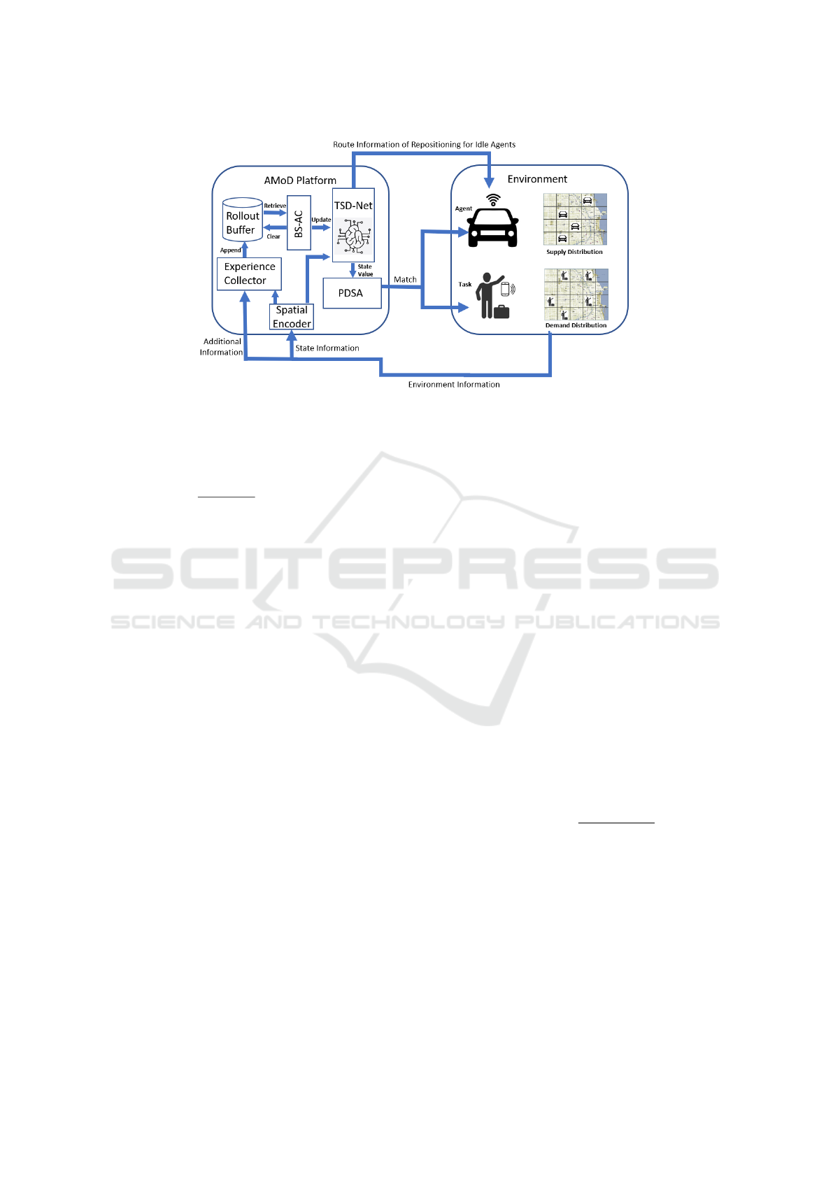
Figure 1: Autonomous Mobility on Demand (AMoD) System.

−→

] is the number of available agents and

−→

] is

the number of tasks at grid cell g

is the grid cell

that the ith available agent moves into at time t).







1 −

−→

]−

−→

]

−→

]

if assigned a task

−1 otherwise

(1)

State Transition. The state transition s

t+1

P (s

) speciﬁes what state the ith available agent

will be in at time t, based on current state s

and ac-

tion a

. In the MDP, there are two types of transitions:

t+1

will be NULL if the agent is assigned a task; oth-

erwise s

t+1

= [

−→

t+1

−→

t+1

Discount Factor. The discount factor γ ∈ [0, 1]

speciﬁes the impact degree of the future rewards. If

γ = 0, an agent is myopic and no future rewards are

taken into account; on the other hand, all future re-

wards have the same weight as the current one if

γ = 1.

The goal of the MDP is to maximize the long term

beneﬁts of each agent, which can be represented by

V (s

) =

∑

t=T

t−T

· r

where T

is the current time.

5 METHODOLOGY

5.1 Temporal-Spatial Dispatching

Network

The architecture of the Temporal-Spatial Dispatch-

ing Network (TSD-Net) is shown in Fig.2. Since the

spatial information has time series property, we de-

sign the Spatial Encoder (SE) with the Gated Recur-

rent Unit (GRU) (Cho et al., 2014) where the hid-

den state h

t−1

involving previous spatial information

is taken as one of inputs (here h

t−1

represents both

t−1

and h

t−1

in the ﬁgure). The purpose of the SE

is to learn the representation of spatial distributions.

To save computational resources, the TSD-Net plays

the role of both policy network (Actor) and value

network (Critic), sampling appropriate actions a

for

each available agent and outputting the scale of the

state value function V (s

,θ) (Sutton and Barto, 2018)

at each time t.

The Norm function within the SE normalizes the

vector of the spatial distribution, as shown in Eq.(2),

where ⃗x

is the input of the function, e.g. the spatial

distribution vector

−→

and

−→

. There are two reasons

for using the Norm function. (i) During rush hours,

most tasks and agents converge around downtown ar-

eas while almost none can be found in non-busy re-

gions, meaning that many elements of vector ⃗x

are 0,

which would cause inefﬁciency in the learning pro-

cess. The Norm function can help get rid of most

zeros. (ii) The close range of the normalized vector ⃗x

improves he sensitivity of the network. Note that the

output of Norm is all-ones vector if std(⃗x

) = 0.

Norm(⃗x

) =

⃗x

− mean(⃗x

)

std(⃗x

)

(2)

Using the properties of time series of spatial data,

the Gated Recurrent Unit (GRU) can combine previ-

ous corresponding information to the present task, as

shown in Eq.(3) where input ⃗y

can be seen as the out-

put of the Norm function and hidden state h

t−1

is the

output of the GRU at time t − 1. The GRU is the vari-

ant version of the LSTM (Hochreiter and Schmidhu-

ber, 1997) which successfully solves the ’long term

dependency’ problem in the Recursive Neural Net-

work (Bengio et al., 1994). When comparing the

Multiple Agents Dispatch via Batch Synchronous Actor Critic in Autonomous Mobility on Demand Systems

201

Figure 2: Temporal-Spatial Dispatching Network (TSD-Net) Architecture.

GRU with the LSTM, it is evident that the GRU ex-

hibits a more compact model structure while retaining

its desirable properties.

= GRU (⃗y

t−1

) (3)

The overall operations of the spatial encoding is

shown in Eq.(4) where W represents parameters of

Linear Layer such as W

or W

′

and ∗ is the matrix

multiplication. In this context, we have devised two

distinct Spatial Encoders (SE) to independently pro-

cess task-related and agent-speciﬁc information. The

primary objective of these SEs is to convert spatial

data into a representative vector encompassing vari-

ous spatial distribution features, integrating it with the

latest temporal learning outcomes through the utiliza-

tion of the GRU.

SE(⃗x

) = W ∗ GRU(Norm(⃗x

),h

t−1

) (4)

As shown in Fig.2, the encoded state vector X

ag-

gregates information of spatial distribution from the

SE and the ith available agent location from One

Hot Encoder at time t, as shown in Eq.(5) where

⊕ is a concatenation operator and Ω symbolizes the

One Hot Encoder which converts categorical data

into binary vectors with a ”1” for the active category

and ”0”s elsewhere. The purpose of the concatena-

tion operation is to bring together global information

(SE(

−→

),SE(

−→

)) and local information (Ω(g

)). This

integration provides subsequent neural network layers

with a rich set of learn-able features for policy train-

ing.

= SE(

−→

) ⊕ SE(

−→

) ⊕ Ω(g

) (5)

The state value V (s

,θ) can be computed by

Eq.(6), where θ is the set of parameters of the TSD-

Net. The V (s

,θ) speciﬁes the expected accumu-

lated rewards starting from state s

. It functions as a

’Critic,’ evaluating whether the current state, denoted

as s

, is advantageous or detrimental for the agents.

This assessment can be leveraged to ﬁne-tune the pol-

icy distribution during training, and also provide ad-

ditional assistance in enabling Autonomous Vehicles

(AVs) to prioritize valuable tasks when supply falls

short.

V (s

,θ) = W

∗ ReLu



∗ ReLu(W

∗ X

)



(6)

Similarly, the action sampling distribution

π(a

,θ) can be computed by Eq.(7), where the

elements of⃗y represent the scores of each action in A

and k = |A

|. This sampling mechanism serves a dual

purpose, preventing both the repetition of the same

actions by AVs in the same area and the convergence

to local optima in the training policy.

⃗y = W

∗ ReLu



∗ ReLu(W

∗ X

)



π(a

,θ) =

⃗y[a

]

∑

⃗y[k]

(7)

5.2 Batch Synchronous Actor Critic

The Actor-Critic algorithm (Konda and Tsitsiklis,

1999) is a kind of Reinforcement Learning (Sutton

and Barto, 2018) that integrates both policy-base and

value-base approaches. The Actor learns an appropri-

ate policy to adapt to the environment while the Critic

evaluates the quality of the learning policy. In this pa-

per, we propose the Batch Synchronous Actor Critic

(BS-AC) of which the basic idea is to train the set of

parameters θ of the TSD-Net with experiences from

the Rollout Buffer, such that the unbiased state value

function V (s

,θ) (Critic) and the appropriate policy

distribution (Actor) can be learned.

Unlike the Advantage Actor Critic (Mnih et al.,

2016) that trains only one agent with all experiences

at each iteration, the BS-AC trains multiple agents

ICAART 2024 - 16th International Conference on Agents and Artiﬁcial Intelligence

202

by sampling a batch of experiences from the Rollout

Buffer with replacement. There are two beneﬁts of

sampling experience with replacement compared to

using the sum of experiences: (i) States that are com-

mon among agents will take priority such that scenar-

ios corresponding to these states can be learned by

agents efﬁciently; (ii) experiences can be reproduced

by sampling with replacement such that the number

of learning experiences can be larger than the number

of experiences in the Rollout Buffer, and sufﬁcient ex-

periences can help agents gain a deeper understanding

of their interactions with the environment.

The Critic V (s

,θ) is learned by minimizing the

following loss function L

(θ), as shown in Eq.(8)

where r

+V (s

t+1

,θ) is the target value to be learned.

(θ) = E



+V (s

t+1

,θ) −V (s

,θ)



(8)

The policy of Actor π(a|s,θ) can be learned by

maximizing the following objective function J

(θ), as

shown in Eq.(9) where p(s) is the probability distribu-

tion of state s under policy π

and A is the Advantage

function. We utilize the Advantage function rather

than state value function V because V would intro-

duce high variance, and A = r

+V (s

t+1

,θ)−V (s

,θ).

(θ) =

∑

s∈S

p(s)

∑

a∈A

π(a|s,θ) · A (9)

Since our neural network architecture TSD-Net

shares parameters between the policy of Actor π

and

the state value function of Critic V , the total objec-

tive function J

a+c

(θ) should combine both J

(θ) and

(θ), as shown in Eq.10. The J

a+c

(θ) is also fur-

ther augmented by the policy entropy H(π

) ensuring

that agents at the same grid cell can still have diversity

movement. Both c

and c

are the constant value.

a+c

(θ) = J

(θ) −c

(θ) + c

H(π

) (10)

where the policy entropy H(π

) is represented by the

formula shown in Eq.11. As shown in the equation,

when the action probabilities of policy π are similar,

the entropy is higher, and vice versa.

H(π

) = −

∑

a=1

π(a,θ) log(π(a, θ)) (11)

The details of the BS-AC training algorithm is

shown in Algo.1. First, each available agent executes

its action to interact with the environment and store its

transition (experience) to the Rollout Buffer D (line

3-10). Then a batch of transitions B is sampled from

D with replacement and the accumulated objective

J is computed from the batch (line 11-16). Finally,

we update the parameters θ of the TSD-Net by the

stochastic gradient ascent and clean up all transitions

in D afterwards (line 17-20).

Algorithm 1: BS-AC Training Algorithm.

1 Initialize a set D as Rollout Buffer.

2 Create the TSD-Net with random parameters

θ.

3 for t = 1 to T

max

4 for each agent ag

in A do

5 if ag

in idle mode then

6 Sample an action a

from the

TSD-Net under state s

7 Execute action a

, observe reward

and next state s

t+1

8 Store transition (s

t+1

) as

an experience into D.

9 end

10 end

11 Sample a batch of transitions B from D

with replacement.

12 J = 0

13 for i = 1 to |B| do

14 Compute the total objective J

a+c

(θ).

15 J = J + J

a+c

(θ)

16 end

17 Perform the Stochastic Gradient Ascent

on J with respect to θ.

18 Update parameters θ = θ + α

|B|

▽

J .

19 Clean up all transitions in D.

20 end

5.3 Priority Destination Sampling

Assignment

To mitigate extended response times, many prior

AMoD systems have employed a First Come First

Serve (FCFS) task assignment strategy, particularly

within the same grid cell. This approach proves ef-

fective when supply meets demand adequately. How-

ever, when supply falls short of demand, tasks with

destinations in remote, low-activity areas tend to

stress the limited supply. Remote destinations neces-

sitate AVs to invest signiﬁcant time in returning to

high-demand regions. If waiting times surpass a cus-

tomer’s patience threshold, they may abandon the ser-

vice. To address this challenge, we introduce the Pri-

ority Destination Sampling Assignment (PDSA) as a

solution for guiding agents to select appropriate tasks

when supply falls short. The fundamental concept be-

hind PDSA is to prioritize each task based on its state

value V (s

,θ) derived from the TSD-Net. Tasks are

subsequently sampled according to their priority val-

ues. This approach increases the likelihood of AVs se-

lecting high-value tasks and being dispatched to desti-

nations with high demand. Simultaneously, tasks with

Multiple Agents Dispatch via Batch Synchronous Actor Critic in Autonomous Mobility on Demand Systems

203

less favorable destinations maintain a chance of being

served, thus preventing potential service gaps. The

sampling distribution is constructed as following:

Pr[τ

] =

p(τ

)

∑

j=1

p(τ

)

(12)

where Pr[τ

] is the probability that task τ

can be sam-

pled, function p indicates priority of τ

, which is de-

termined by the order rank of the state value, κ spec-

iﬁes the total number of tasks in grid cell where τ

locates, and µ ∈ [0, 1] is a factor suggesting the degree

of the priority used. The advantage of the PDSA is

that tasks with ’hot’ destinations have better chances

to be served while tasks with ’cold’ destinations will

still not be ignored completely.

The details of the PDSA algorithm are shown in

Algo.2. First, we still follow the FSFC strategy if the

number of agents is greater than tasks (Line 1-2). If

not, the priority of each task is computed by its order

rank based on the state value from the Critic of the

TSD-Net (Line 4-5). Finally, an appropriate task is

sampled by probability Pr[τ

] and assigned to an agent

(Line 6-9).

Algorithm 2: PDSA Algorithm.

Input: The agent set A(g

) and the task set

T (g

) at grid g

1 if |A(g

)| ≥ |T (g

)| then

2 return

3 else

4 Sort tasks in T (g

) based on the state

value of their destination by descending

order.

5 Compute each task’s priority by its rank

in the sorted set, p(τ

) =

rank(τ

)

6 for each agent ag

in A(g

) do

7 Sample task τ

∼ Pr[τ

8 Assign task τ

to agent ag

9 end

10 end

6 EXPERIMENT

6.1 Experimental Setup

Evaluation Data. Our experiments are based on a

real world city-scale dataset from the City of Chicago

during September in 2019 (Chicago, 2018), which

contains about 1.3 million records. Each record repre-

sents as a task in our AMoD System contains a num-

ber of attributes: record ID, starting time, origin, des-

tination, trip time and total trip fee.

To evaluate the effectiveness, scalability and ro-

bustness of our approach, three time periods are se-

lected, and their time temporal patterns are shown in

Fig.3. In the morning (Fig.3a), we observe that the

average number of tasks per minute increases steadily

to 50 at 9:00AM, peaking at more than 60 tasks per

minute, and ﬂuctuating around 45 tasks per minute af-

terwards. At noon (Fig.3b), the average of the number

of tasks seems relatively stable, going up and down

between 40 and 50. The evening period is more chal-

lenging (Fig.3c). The peak of tasks per minute is

greater than 70, and then the amount decreases dra-

matically after 19:00PM.

The spatial patterns for these three time periods

are depicted in Figure 4. In the city’s hotspots (Fig-

ure 4a), zones 8, 28, 32, and 33 represent the down-

town areas, while zone 76 corresponds to the airport.

Typically, across downtown areas, the volume of tasks

during noon and evening notably surpasses that of the

morning, with the exception of zone 28, where the

task volume in the morning is slightly higher. This

phenomenon is primarily because few businesses and

activities occur in downtown areas during the morn-

ing. A similar trend is observed at the airport. Con-

versely, in the city’s common areas (Figure 4b), the

differences in task distribution across the three time

periods within each zone are less pronounced. During

the morning, tasks are more evenly distributed. This

is because residents from various neighborhoods re-

quest AVs in the morning, leading to a more balanced

task distribution across the city.

Comparison Methods. Our approach is com-

pared with the following baselines in terms of Service

Rate, Response Time, and Repositioning Time.

• Random. The available agents stochastically se-

lect one of the neighboring grid cells or current

grid cell for their relocation. This method serves

as the lower bound of the comparison.

• Soft S-D Heuristic. Based on the information of

task and agent distribution, the Soft S-D heuristic

directs AVs to locations which are generally pop-

ular, without regard to time of day. This method

is robust to the environmental parameter change.

• AS-DDQN (Zheng et al., 2022). Using the di-

rection scores obtained from the Double Deep-

Q-Network (DDQN), agents sample an appropri-

ate direction to execute. Directions with higher

scores are more likely to be chosen. This method

can discourage all AVs who are in the same places

from making the same decision.

ICAART 2024 - 16th International Conference on Agents and Artiﬁcial Intelligence

204

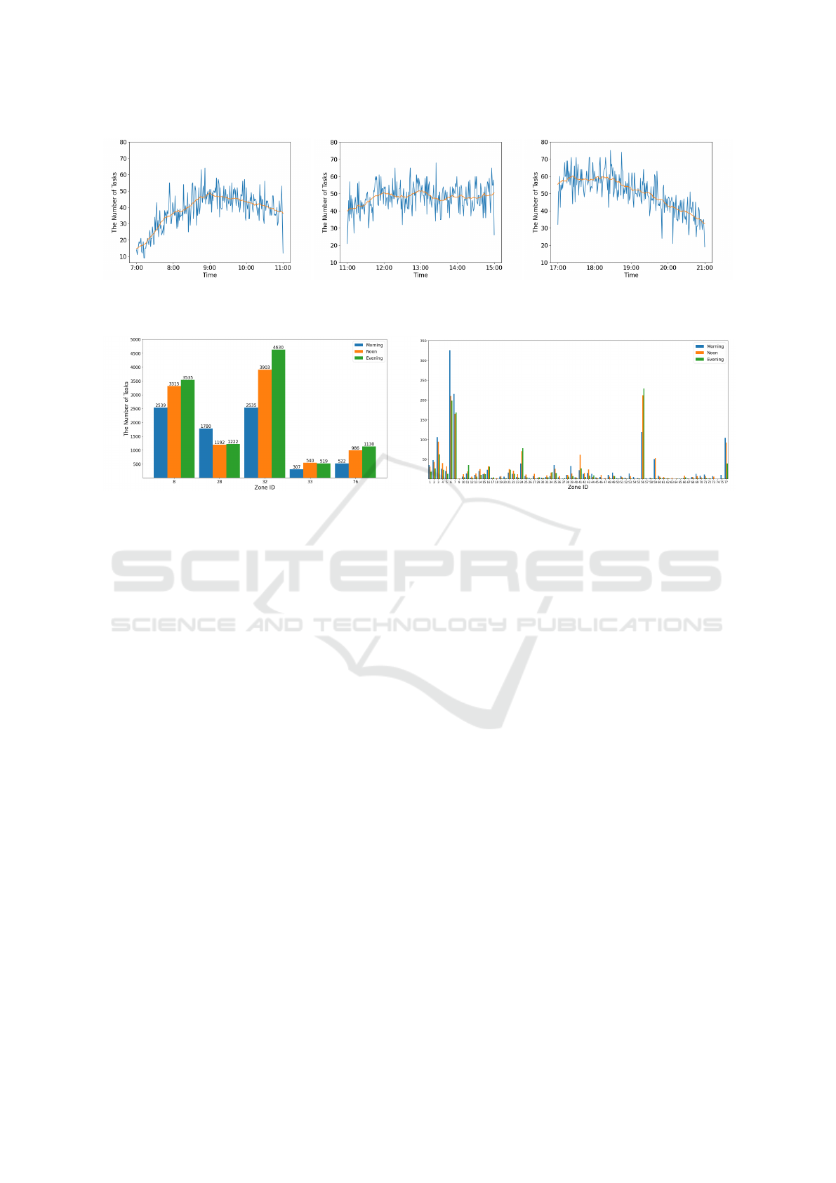
(a) Morning. (b) Noon. (c) Evening.

Figure 3: Temporal patterns of three time periods. The blue line represents real time tasks amount tracked by every minute

while the orange line speciﬁes the average tasks amount within 15 minutes.

(a) Downtown and airport areas. (b) Other areas.

Figure 4: Spatial patterns of three time periods. The X-axis represents zone ID of the city, while Y-axis stands for the total

tasks amount in each time period separately.

• Soft cDQN (Lin et al., 2018). Agents make

decisions with output from the Deep-Q-Network

(DQN) and the context information of the envi-

ronment and the deployment of other agents. This

method can reduce the dimension of agents’ ac-

tion space and make the learning process effec-

tive.

• Ours. Our approach utilizes a novel neural net-

work framework, an improved learning process,

and a considerable task assignment mechanism to

make agents more sensitive and adaptive to the

dynamic properties of the environment.

Deployment. The city is partitioned into 77 cells.

The simulation cycle is set to be 1 minute and the

patience duration of passengers is assumed to be 10

minutes during the comparison. To further challenge

the simulation, the initial locations of all agents are

remote areas where tasks rarely occurs. In terms of In

our approach, the batch size is set to be 1024. The dis-

count factor γ = 0.99. The learning rate is α = 0.0005,

and constant value c

= 0.5, c

= 0.001.

6.2 Performance Measurements

In this work, the performance of the AMoD System is

evaluated by the following measurements.

Measurement 1: Service Rate. The Served Rate

measures the proportion of tasks that can be served by

agents in the AMoD System successfully.

Measurement 2: Response Time. The Response

Time estimates the average time duration between

rider request and pickup by an AV.

Measurement 3: Repositioning Time. The

Repositioning Time gauges the average relocation

time between when an agent completes one task and

ﬁnds another to serve.

6.3 Performance Comparison

To verify the effectiveness, scalability and robustness

of our proposed approach, we compare it with other

competitive baseline methods in terms of Service

Rate, Response Time and Repositioning Time along

with various numbers of agents within three time pe-

riods: Morning(7AM∼11AM), Noon(11AM∼3PM)

and Evening(5PM∼9PM), as shown in Fig.5. Gener-

ally, more agents means more tasks can be handled,

less tasks’ responsive time while more repositioning

time for agents themselves. In particular, several ob-

servations are made from Fig.5 as following:

1. Compared to the Random method, the Soft SD-

Heuristic attains improved results over all perfor-

mance measurements. This is because the Soft

SD-Heuristic can intentionally diffuse agents to

local areas where supply is insufﬁcient for de-

mand.

Multiple Agents Dispatch via Batch Synchronous Actor Critic in Autonomous Mobility on Demand Systems

205

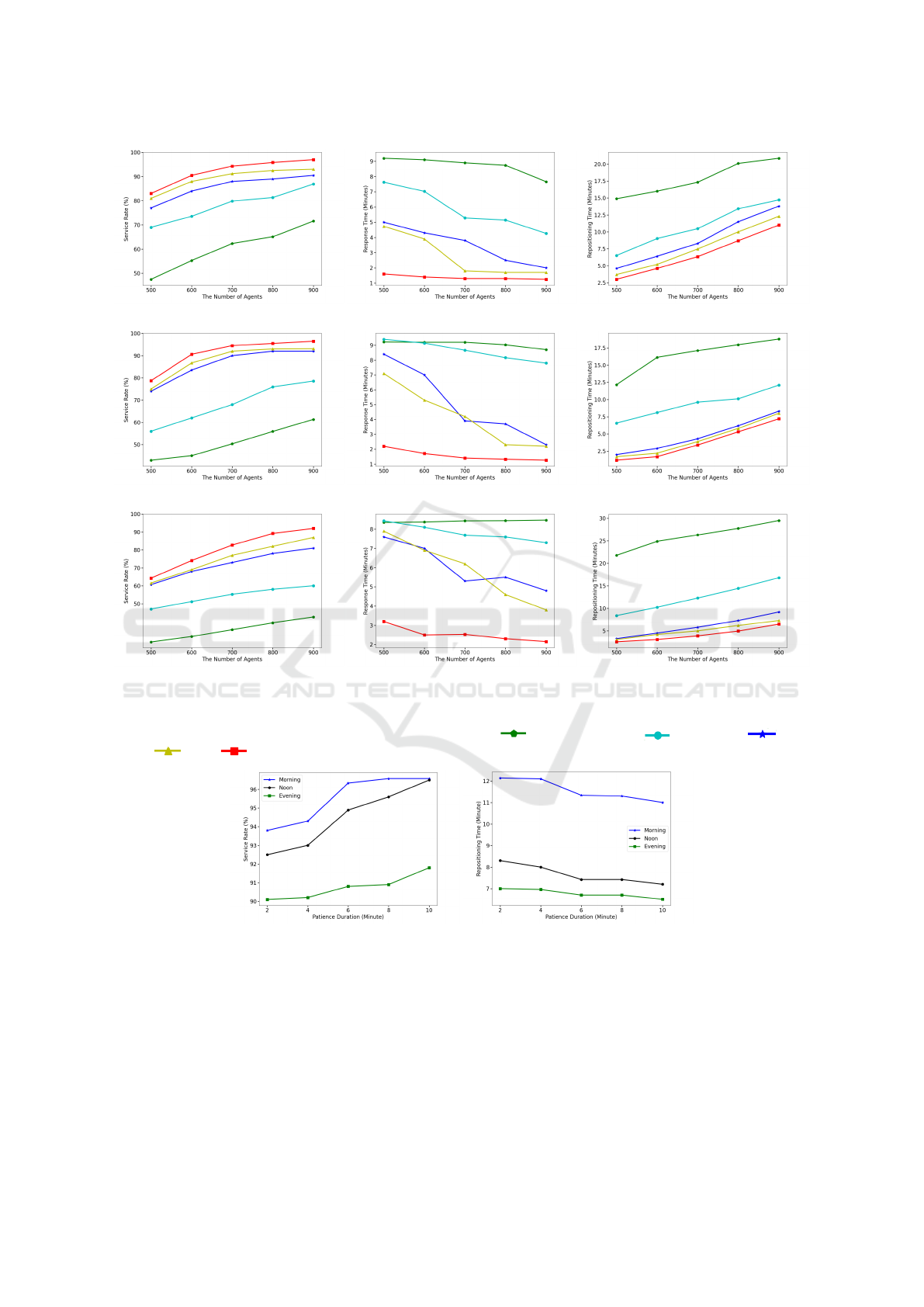
(a) Service Rate (Morning). (b) Response Time (Morning). (c) Repositioning Time (Morning).

(d) Service Rate (Noon). (e) Response Time (Noon). (f) Repositioning Time (Noon).

(g) Service Rate (Evening). (h) Response Time (Evening). (i) Repositioning Time (Evening).

Figure 5: Performance Comparisons of competitive approaches w.r.t. Service Rate, Response Time and Reposition-

ing Time along with various number of agents within three time periods: Morning(7AM∼11AM), Noon(11AM∼3PM)

and Evening(5PM∼9PM). The graph key is as follows: Random: , Soft SD-Heuristic: , AS-DDQN: , Soft

cDQN: , Ours: .

(a) Service Rate. (b) Repositioning Time.

Figure 6: The robustness tests of the Service Rate and the Repositioning Time along with various patience duration of

passengers.

2. The learning based methods make signiﬁcant im-

provement upon the heuristic method because the

learning approaches seek to optimize the long

term beneﬁt while the heuristic maintains a my-

opic focus on the current beneﬁt. Also, the learn-

ing based methods consider the spatial distribu-

tion of agents and tasks globally while the heuris-

tic only cares about supply and demand locally.

3. With respect to the learning based method, the se-

ries algorithms of actor critic outperform the DQN

series. There are two reasons for this: (i) the Q

value approximator of the DQN is not guaranteed

to converge while the policy approximator of the

ICAART 2024 - 16th International Conference on Agents and Artiﬁcial Intelligence

206

actor critic has better convergence properties; (ii)

the actor critic algorithms use policy entropy to

ensure the diversity of action samples each time,

but the DQN will eventually tend to select the ac-

tion with highest Q value, even though the soft-

max function is used.

4. In terms of the DQN series, the Soft cDQN is

somewhat better than the AS-DDQN, the main

reason being that the AS-DDQN uses the rank as

a priority that is rigid for the action distribution

such that it is difﬁcult to adapt to the dynamic of

the environments.

5. We observe that our approach outperforms other

baselines.This is mainly because the TSD-Net uti-

lizes the GRU to process the spatial information

with temporal signals such that accurate repre-

sentation features can be learned; moreover, the

PDSA can effectively allocate agents to suitable

areas by prioritizing tasks with destinations in

high-demand areas. This arrangement ensures

that agents are consistently in proximity whenever

a high-demand task becomes available.

With 900 agents and our approach, the perfor-

mances of the Service Rate and the Repositioning

Time applying various patience durations of cus-

tomers are shown in Fig.6. In terms of the Service

Rate, we observe that the ﬂuctuation in the morning

and noon is within 3% while in the evening no more

than 1%. On the other hand, for the Repositioning

Time, the performance changes over all three time pe-

riods are within 1 minute. From this perspective, our

approach is robust and adaptive with various patience

duration settings.We also observe that Autonomous

Vehicles (AVs) spend more time repositioning dur-

ing the morning hours in comparison to the noon and

evening periods. This disparity can be attributed to

the following factors: (i) In hotspot areas, task de-

mand during noon and evening is notably higher than

in the morning, as illustrated in Figure 4a. Conse-

quently, most AVs working during these periods do

not need to invest signiﬁcant time in repositioning, as

they continue to have ample opportunities primarily

within the downtown and airport regions. (ii) Un-

like the concentrated task distribution in hotspot ar-

eas during noon and evening, task distribution in the

morning tends to be more evenly dispersed across the

city, as depicted in Figure 4. AVs are compelled to

allocate additional time during the morning to reach

customers before being assigned tasks. Conversely,

tasks in business districts are more prevalent during

the noon and evening hours and are typically concen-

trated in downtown areas. This concentration allows

AVs to reduce the time needed to reach these tasks,

thereby minimizing repositioning requirements.

7 CONCLUSION

In this paper, there are four contributions to AMoD

systems. First, the TSD-Net combines both policy

and value networks to save computational cost. It

also facilitates the temporal signals behind spatial in-

formation to learn representation features. Second,

to decrease time needed to collect experiences, the

BS-AC algorithm samples experience from the Roll-

out Buffer with replacement and utilizes Stochastic

Gradient Ascent to train the parameters of TSD-Net.

Thirdly, based on the state value from the Critic of

the TSD-Net, the PDSA algorithm deﬁnes priorities

of each task and samples appropriate ones for agents.

Finally, performance comparisons are conducted to

verify the effectiveness, scalability and robustness of

our approach.

While the proposed Multiagent Reinforcement

Learning (MARL) framework has demonstrated sig-

niﬁcant performance improvements in the ﬁeld of

AMoD systems, several limitations remain that need

to be addressed in the future:

• The TSD-Net considers correlations in terms of

temporal patterns but overlooks interactions con-

cerning spatial patterns. For instance, certain grid

cells adjacent to high-demand activity areas such

as downtown or airports may exhibit sparse de-

mand themselves. However, deploying agents

around these areas might prove to be a strate-

gic choice. Leveraging Graph Neural Networks

(GNNs) (Sanchez-Lengeling et al., 2021) presents

a promising approach to processing spatial in-

formation within a graph framework. Future re-

search endeavors should focus on exploring meth-

ods to integrate GNNs into the existing TSD-Net,

enabling a more comprehensive consideration of

spatial aspects.

• In regions with low supply where agents seldom

operate, their decision-making can suffer due to

insufﬁcient experience to train the policy network.

Consequently, satisfying demands in these areas

becomes challenging, potentially leading to inef-

ﬁcient behavior by agents. Future research aims

to investigate methods enabling machines to gen-

erate experiences automatically corresponding to

low-supply areas. This exploration intends to fa-

cilitate proper training of the policy network, ulti-

mately enhancing the decision-making process in

underrepresented regions.

Multiple Agents Dispatch via Batch Synchronous Actor Critic in Autonomous Mobility on Demand Systems

207

REFERENCES

Bengio, Y., Simard, P., and Frasconi, P. (1994). Learning

long-term dependencies with gradient descent is difﬁ-

cult. IEEE transactions on neural networks, 5(2):157–

166.

Chicago (2018). Chicago Data Portal: Taxi Trips.

https://data.cityofchicago.org/Transportation/

Taxi-Trips/wrvz-psew.

Cho, K., van Merri

enboer, B., Gulcehre, C., Bahdanau, D.,

Bougares, F., Schwenk, H., and Bengio, Y. (2014).

Learning phrase representations using RNN encoder–

decoder for statistical machine translation. In Mos-

chitti, A., Pang, B., and Daelemans, W., editors, Pro-

ceedings of the 2014 Conference on Empirical Meth-

ods in Natural Language Processing (EMNLP), pages

1724–1734, Doha, Qatar. Association for Computa-

tional Linguistics.

Gammelli, D., Yang, K., Harrison, J., Rodrigues, F.,

Pereira, F. C., and Pavone, M. (2022). Graph

meta-reinforcement learning for transferable au-

tonomous mobility-on-demand. arXiv preprint

arXiv:2202.07147.

Hochreiter, S. and Schmidhuber, J. (1997). Long short-term

memory. Neural computation, 9(8):1735–1780.

Konda, V. and Tsitsiklis, J. (1999). Actor-critic algorithms.

Advances in neural information processing systems,

12.

Krizhevsky, A., Sutskever, I., and Hinton, G. E. (2017). Im-

agenet classiﬁcation with deep convolutional neural

networks. Communications of the ACM, 60(6):84–90.

Li, J. and Allan, V. H. (2022a). T-balance: A uniﬁed mech-

anism for taxi scheduling in a city-scale ride-sharing

service. In ICAART (2), pages 458–465.

Li, J. and Allan, V. H. (2022b). Where to go: Agent guid-

ance with deep reinforcement learning in a city-scale

online ride-hailing service. In 2022 IEEE 25th In-

ternational Conference on Intelligent Transportation

Systems (ITSC), pages 1943–1948. IEEE.

Lin, K., Zhao, R., Xu, Z., and Zhou, J. (2018). Efﬁcient

large-scale ﬂeet management via multi-agent deep re-

inforcement learning. In Proceedings of the 24th

ACM SIGKDD International Conference on Knowl-

edge Discovery & Data Mining, pages 1774–1783.

Lin, L.-J. (1992). Reinforcement learning for robots using

neural networks. Carnegie Mellon University.

Mnih, V., Badia, A. P., Mirza, M., Graves, A., Lillicrap, T.,

Harley, T., Silver, D., and Kavukcuoglu, K. (2016).

Asynchronous methods for deep reinforcement learn-

ing. In International conference on machine learning,

pages 1928–1937. PMLR.

Mnih, V., Kavukcuoglu, K., Silver, D., Graves, A.,

Antonoglou, I., Wierstra, D., and Riedmiller, M.

(2013). Playing atari with deep reinforcement learn-

ing. arXiv preprint arXiv:1312.5602.

Mnih, V., Kavukcuoglu, K., Silver, D., Rusu, A. A., Ve-

ness, J., Bellemare, M. G., Graves, A., Riedmiller, M.,

Fidjeland, A. K., Ostrovski, G., et al. (2015). Human-

level control through deep reinforcement learning. na-

ture, 518(7540):529–533.

Munkres, J. (1957). Algorithms for the assignment and

transportation problems. Journal of the society for in-

dustrial and applied mathematics, 5(1):32–38.

Sanchez-Lengeling, B., Reif, E., Pearce, A., and Wiltschko,

A. B. (2021). A gentle introduction to graph neural

networks. Distill. https://distill.pub/2021/gnn-intro.

Schaul, T., Quan, J., Antonoglou, I., and Silver, D.

(2015). Prioritized experience replay. arXiv preprint

arXiv:1511.05952.

Schulman, J., Wolski, F., Dhariwal, P., Radford, A., and

Klimov, O. (2017). Proximal policy optimization al-

gorithms. arXiv preprint arXiv:1707.06347.

Sun, J., Jin, H., Yang, Z., Su, L., and Wang, X. (2022).

Optimizing long-term efﬁciency and fairness in ride-

hailing via joint order dispatching and driver reposi-

tioning. In Proceedings of the 28th ACM SIGKDD

Conference on Knowledge Discovery and Data Min-

ing, pages 3950–3960.

Sutton, R. S. and Barto, A. G. (2018). Reinforcement learn-

ing: An introduction. MIT press.

Sutton, R. S., McAllester, D., Singh, S., and Mansour, Y.

(1999). Policy gradient methods for reinforcement

learning with function approximation. Advances in

neural information processing systems, 12.

Tesauro, G. et al. (1995). Temporal difference learning and

td-gammon. Communications of the ACM, 38(3):58–

68.

UN, D. (2015). World urbanization prospects: The 2014

revision. United Nations Department of Economics

and Social Affairs, Population Division: New York,

NY, USA, 41.

Van Hasselt, H., Guez, A., and Silver, D. (2016). Deep re-

inforcement learning with double q-learning. In Pro-

ceedings of the Thirtieth AAAI Conference on Artiﬁ-

cial Intelligence, AAAI’16, page 2094–2100.

Wang, G., Zhong, S., Wang, S., Miao, F., Dong, Z., and

Zhang, D. (2021). Data-driven fairness-aware vehi-

cle displacement for large-scale electric taxi ﬂeets. In

2021 IEEE 37th International Conference on Data

Engineering (ICDE), pages 1200–1211. IEEE.

Wang, Z., Qin, Z., Tang, X., Ye, J., and Zhu, H. (2018).

Deep reinforcement learning with knowledge transfer

for online rides order dispatching. In 2018 IEEE Inter-

national Conference on Data Mining (ICDM), pages

617–626. IEEE.

Wang, Z., Schaul, T., Hessel, M., Hasselt, H., Lanctot, M.,

and Freitas, N. (2016). Dueling network architec-

tures for deep reinforcement learning. In International

conference on machine learning, pages 1995–2003.

PMLR.

Wen, J., Zhao, J., and Jaillet, P. (2017). Rebalancing shared

mobility-on-demand systems: A reinforcement learn-

ing approach. In 2017 IEEE 20th international con-

ference on intelligent transportation systems (ITSC),

pages 220–225. Ieee.

Xu, Z., Li, Z., Guan, Q., Zhang, D., Li, Q., Nan, J., Liu,

C., Bian, W., and Ye, J. (2018). Large-scale order dis-

patch in on-demand ride-hailing platforms: A learning

and planning approach. In Proceedings of the 24th

ICAART 2024 - 16th International Conference on Agents and Artiﬁcial Intelligence

208

ACM SIGKDD International Conference on Knowl-

edge Discovery & Data Mining, pages 905–913.

Zheng, B., Ming, L., Hu, Q., L

u, Z., Liu, G., and Zhou,

X. (2022). Supply-demand-aware deep reinforcement

learning for dynamic ﬂeet management. ACM Trans-

actions on Intelligent Systems and Technology (TIST),

13(3):1–19.

Multiple Agents Dispatch via Batch Synchronous Actor Critic in Autonomous Mobility on Demand Systems

209