Evaluating Quantum Support Vector Regression Methods

for Price Forecasting Applications

Horst Stühler

1 a

, Daniel Pranji

2 b

and Christian Tutschku

2 c

Zeppelin GmbH, Graf-Zeppelin-Platz 1, 85766 Garching, Germany

Fraunhofer IAO, Nobelstraße 12, 70569 Stuttgart, Germany

Keywords:

Price Forecasting, Machine Learning, ML, Quantum Machine Learning, QML, SVR, QSVR.

Abstract:

Support vector machines are powerful and frequently used machine learning methods for classiﬁcation and

regression tasks, which rely on the construction of kernel matrices. While crucial for the performance of this

machine learning approach, choosing the most suitable kernel is highly problem-dependent. The emergence

of quantum computers and quantum machine learning techniques provides new possibilities for generating

powerful quantum kernels. Within this work, we solve a real-world price forecasting problem using ﬁdelity and

projected quantum kernels, which are promising candidates for the utility of near-term quantum computing. In

our analysis, we examine and validate the most auspicious quantum kernels from literature and compare their

performance with an optimized classical kernel. Unlike previous work on quantum support vector machines,

our dataset includes categorical features that need to be encoded as numerical features, which we realize by

using the one-hot-encoding scheme. One-hot-encoding, however, increases the dimensionality of the dataset

signiﬁcantly, which collides with the current limitations of noisy intermediate scale quantum computers. To

overcome these limitations, we use autoencoders to learn a low-dimensional representation of the feature space

that still maintains the most important information of the original data. To examine the impact of autoencoding,

we compare the results of the encoded date with the results of the original, unencoded dataset. We could

demonstrate that quantum kernels are comparable to or even better than the classical support vector machine

kernels regarding the mean absolute percentage error scores for both encoded and unencoded datasets.

1 INTRODUCTION

Machine learning (ML) methods of any kind are

used to generate satisfying and reliable price fore-

casting applications for different use cases and indus-

tries. One example is the sector of heavy construc-

tion equipment dealers that rely heavily on accurate

price predictions. Determining their ﬂeet’s current

and future residual value allows construction equip-

ment dealers to identify the optimal time to resell

individual pieces of machinery (Lucko et al., 2007;

Chiteri, 2018). Using ML methods to calculate the

residual value of construction equipment is of high

interest and has already been tested in the past (Zong,

2017; Chiteri, 2018; Miloševi

c et al., 2021; Shehadeh

et al., 2021; Alshboul et al., 2021; Stühler. et al.,

2023). It has been shown, that the use of existing ML

https://orcid.org/0000-0002-7638-1861

https://orcid.org/0009-0007-5307-7377

https://orcid.org/0000-0003-0401-5333

and automated machine learning (AutoML) methods

generate good results for different applications and

datasets (Zöller et al., 2021; Zoph and Le, 2016; Stüh-

ler. et al., 2023).

Although generating desirable results, these meth-

ods have a strong demand for computational power

needed to create accurate results within a reasonable

runtime. Here is where quantum computers (QCs)

with their promised quantum advantage (Shor, 1999;

Harrow et al., 2009; Huang et al., 2021; Liu et al.,

2021) come into play. The new ﬁeld of quantum ma-

chine learning (QML) based on QCs provides new

possibilities for generating powerful quantum-based

ML applications with better accuracy and less time

and power consumption.

A commonly employed approach in ML for both

classiﬁcation and regression tasks is the Support

vector machine (SVM) (Steinwart and Christmann,

2008). SVMs depend on the creation of kernel matri-

ces. Selecting the most appropriate kernel depends on

the speciﬁc problem at hand, and QML methods pro-

376

Stühler, H., Pranji

c, D. and Tutschku, C.

Evaluating Quantum Support Vector Regression Methods for Price Forecasting Applications.

DOI: 10.5220/0012351400003636

Paper published under CC license (CC BY-NC-ND 4.0)

In Proceedings of the 16th International Conference on Agents and Artiﬁcial Intelligence (ICAART 2024) - Volume 3, pages 376-384

ISBN: 978-989-758-680-4; ISSN: 2184-433X

vide new possibilities for generating potent quantum

kernels (Huang et al., 2021; Thanasilp et al., 2022).

This study uses various ﬁdelity and projected

quantum kernel techniques to address an industrial

price forecasting application (Stühler. et al., 2023).

Our analysis focuses on evaluating the most promis-

ing quantum kernels documented in the literature and

assesses their performance against an optimized clas-

sical SVM kernel. Similar to the work presented in

(Grossi et al., 2022), we use different feature set com-

binations of the dataset to examine the importance of

the features and their impact on the results.

Our work extends previous studies regarding two

novel aspects. (a) In contrast to previous works,

our dataset contains categorical features that require

conversion into numerical features, a task achieved

through the implementation of the one-hot-encoding

method. However, this process substantially aug-

ments the dataset’s dimensionality, which poses a

challenge given the current constraints of noisy in-

termediate scale quantum (NISQ) computers. To ad-

dress this issue, we employ autoencoders (Bank et al.,

2020) to acquire a condensed representation of the

feature space that retains the essential information

from the initial data, as it was also done in the con-

text of anomaly detection with QML in (Wo´zniak

et al., 2023). (b) We extend the latter approach by

not only using ﬁdelity quantum kernels but also pro-

jected quantum kernels (Huang et al., 2021), which

are promising candidates for the utility of near-term

quantum computing schemes. We ﬁnally analyze the

results of the different (Q)SVM methods and compare

the results of the encoded data sets with those of the

original data sets to investigate the impact of autoen-

coders on the entire pipeline.

The work is structured as follows: In section 2, we

present related work. Section 3 describes the method-

ology. The main ﬁndings are presented in Section 4

followed by a conclusion.

2 RELATED WORK

2.1 Machine Learning for Price

Prediction

In order to interpret the results within this paper and

to embed these ﬁndings in the current literature, let

us brieﬂy recap the most related work and their spe-

cial focus. (Zong, 2017) estimates the residual value

of used articulated trucks using various regression

models. Similarly, (Chiteri, 2018) analyses the resid-

ual value of

⁄

ton trucks based on historical data

from auctions and resale transactions. Furthermore,

(Miloševi

c et al., 2021) construct an ensemble model

based on a diverse set of regression models to pre-

dict the residual value of 500 000 construction ma-

chines advertised in the USA. In addition, (Shehadeh

et al., 2021) and (Alshboul et al., 2021) use vari-

ous regression models to predict the residual value of

six construction equipment types based on data from

open-accessed auction databases. Finally, (Stühler.

et al., 2023) compared seven different state-of-the-art

and well-established ML methods with three AutoML

methods on a dataset generated from real online ad-

vertisements, consisting of 2910 datapoints from 10

different Caterpillar models.

All these research activities underline the advan-

tages and necessity of ML methods when dealing with

price forecasting applications.

2.2 Quantum Machine Learning

In the search for an advantage over classical meth-

ods with quantum computing, machine learning is ex-

pected to be one of the ﬁrst ﬁelds to beneﬁt from

quantum computers (Biamonte et al., 2017). Quan-

tum machine learning deals with incorporating quan-

tum algorithms for learning problems. Proven quan-

tum advantages in QML are based on algorithms that

can only be executed on fault-tolerant QCs (Shor,

1999; Harrow et al., 2009; Huang et al., 2021; Liu

et al., 2021). As this ﬁeld just started with the emer-

gence of commercially available NISQ computers,

the practical implementation of the already known al-

gorithms is still in its infancy. There are three rea-

sons why we decided to use quantum support vec-

tor machines (QSVMs): (a) The proven speed-up in

a constructed theoretical problem based on the dis-

crete logarithm (Liu et al., 2021). (b) From a mathe-

matical point of view, classical SVMs are well under-

stood within the statistical learning theory in terms of

error bounds, convergence, robustness, and computa-

tional complexity (Steinwart and Christmann, 2008;

Schölkopf et al., 2002; Vapnik, 1999; Cortes and

Vapnik, 1995). Since for most QSVMs only the

kernel estimation is done on a quantum computer,

there are rigorous error bounds as well (Huang et

al., 2021). (c) QSVMs are especially suitable for the

NISQ era because of their shallow circuits. It should

be noted that the SVM optimization can be formu-

lated as a quadratic unconstrained binary optimiza-

tion (QUBO) problem (Willsch et al., 2020; Cavallaro

et al., 2020) and can hence be solved on a quantum

annealer (Kadowaki and Nishimori, 1998; Das and

Chakrabarti, 2005; Hauke et al., 2020). While this

is its own research branch, we focus on kernel-based

quantum regression in the scope of this paper.

Evaluating Quantum Support Vector Regression Methods for Price Forecasting Applications

377

Clear dataset of duplicates

Remove outliers

Generate dataset with different

feature combinations

Evaluate and document results

for all four feature combination

Train Models

One-hot encoding & scaling

Encoded

Unencoded

QSVR

!"#$

"%#$

QSVR

!"#$

"%#&'%

QSVR

!"#(

"%#&'%

QSVR

!"#(

"%#&'%

QSVR

!"#$

"%#$

QSVR

!"#$

"%#&'%

QSVR

)*+,

QSVR

)*+,

SVR

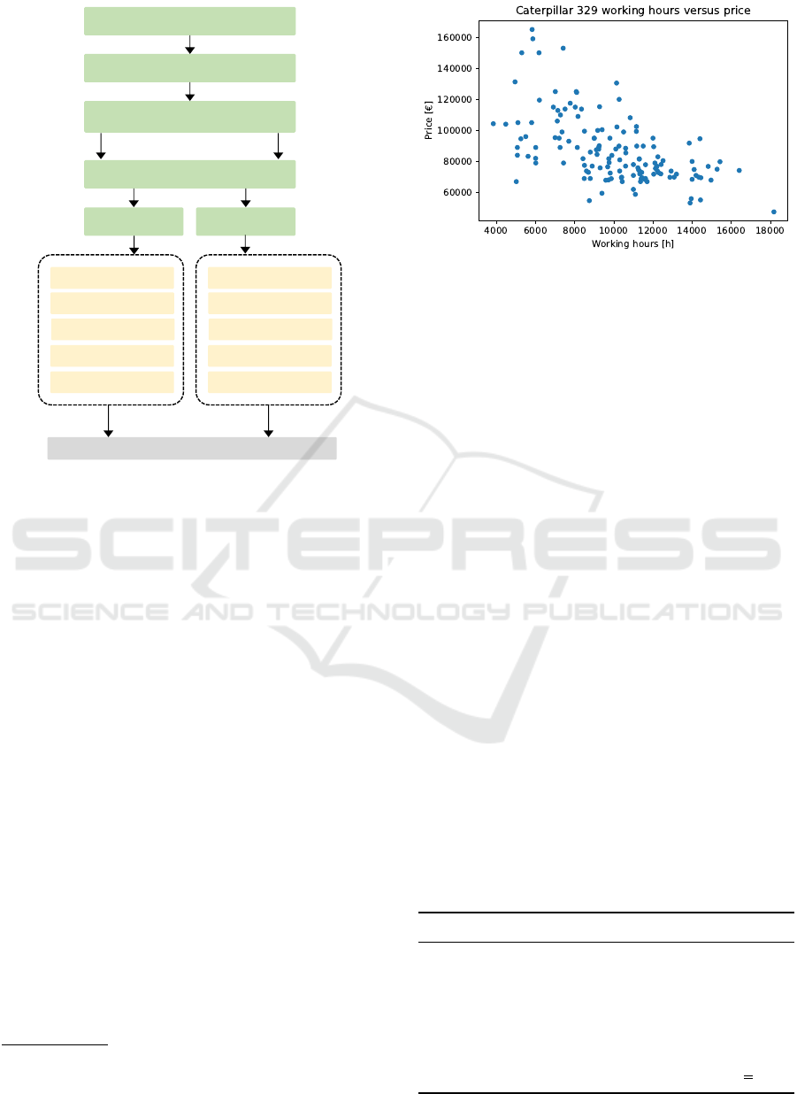
Figure 1: Methodology framework: The case study pipeline

illustrates the steps of the data processing phase in green

and the (Q)SVR algorithms in yellow. QSVR

en=0

re=0

is with-

out entanglement & data re-uploading. QSVR

en=lin

re=0

is with

linear entanglement & no data re-uploading. QSVR

en=lin

re=1

is with entanglement & one data re-uploading.

3 METHODOLOGY

To examine the QML capabilities, we compare four

quantum support vector regression (QSVR) methods,

which will be introduced in chapter 3.4 and chap-

ter 3.5 with a state-of-the-art classical support vec-

tor regression (SVR) implementation, introduced in

chapter 3.3. The overall method and the case study

pipeline are depicted in Figure 1 and explained in the

subsequent sections. The developed source code is

available on GitHub

3.1 Data Creation

The initial data was obtained by regularly collect-

ing all advertisements from seven major construction

equipment market portals

over a time period of seven

months. Table 1 shows the collected and selected fea-

tures.

See https://tinyurl.com/ymmts5xc.

The market portals are Mascus, Catused, Mobile, Ma-

chineryLine, TradeMachines, Truck1, and Truckscout24.

Figure 2: Working hours versus price for the Caterpillar 329

dataset.

Duplicate entries are eliminated by an iterative

comparison of different feature combinations. Out-

liers were detected by a plausibility check, namely

removing values outside a 99% conﬁdence interval,

considering working hours and price.

Dealing with missing values depends on the at-

tribute. Samples are dropped if a value of the fea-

tures model, construction year, extension, or location

is missing. Missing values for the working hours at-

tribute will be substituted via stochastic regression

imputation (Newman, 2014). The entries for brand

and price are mandatory on all portals for creating ad-

vertisements.

In contrast to (Stühler. et al., 2023) for computa-

tional reasons, we only took the dataset of the Cater-

pillar model 329 with 141 data points. The distribu-

tion of the data points concerning the working hours

and price features are depicted in Figure 2. As we

took one machine model manufactured by Caterpillar,

the brand and the model feature, depicted in Table 1,

are thus obsolete. Table 2 shows an excerpt of the re-

sulting dataset. Data subsets with individual feature

combinations are created to account for and investi-

gate the impact of single features. The subset consist-

ing of the working hours and construction year is used

as the baseline feature set (subsequently referred to as

basic subset). In addition, this basic subset was ex-

Table 1: Collected dataset features with types and examples.

Feature Type Example

Brand Categorical Caterpillar

Model Categorical 329

Extension Categorical E

Construction year Numerical 2018

Working hours Numerical 8536

Location Categorical Germany

Price Numerical 59.000 C

ICAART 2024 - 16th International Conference on Agents and Artiﬁcial Intelligence

378

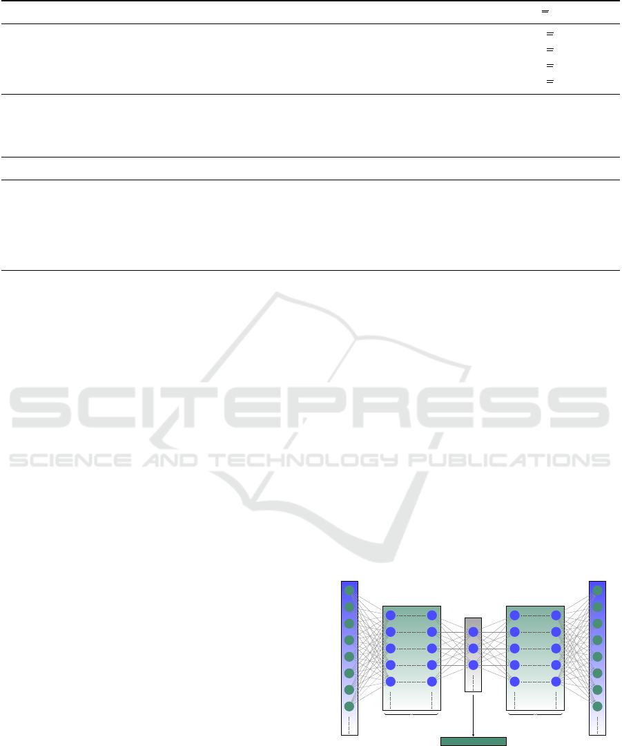
Table 2: Excerpt of the Caterpillar 329 dataset.

Extension Construction year Working hours [h] Location Price [C]

E 2012 10600 DE 77.000 C

D 2008 18180 CH 47.499 C

E 2012 11424 DE 72.900 C

E 2014 11500 DE 89.900 C

Table 3: Feature set combinations with the corresponding input and latent space dimensions. The features working hours &

constructin year form the basic subset and are the basis of all feature set combinations. The maximum size of the latent space

is 10. All feature sets are encoded to guarantee comparability.

Feature set Input size Latent size

basic subset 2

Autoencoded

−−−−−−−→ 2

basic subset + extension 4

Autoencoded

−−−−−−−→ 4

basic subset + location 16

Autoencoded

−−−−−−−→ 10

basic subset + extension + location 18

Autoencoded

−−−−−−−→ 10

tended by the extension and the location features and

all combinations of them, resulting in four data sets.

3.2 Autoencoding

The autoencoder (AE) (Tschannen et al., 2018; Ng

et al., 2011) is an unsupervised learning algorithm

that consists of two neural networks - the encoder and

the decoder (see Figure 3). While the former is used

to encode the input data in a reduced or dense rep-

resentation, called latent representation, the latter is

used to decode the original input from this reduced

representation. One advantage of using an AE is its

ﬂexibility, i.e., the dimensionality of the latent space

representation can be changed by adding or removing

neurons, which is used to generate latent spaces de-

pending on the size or dimensionality of the datasets.

As mentioned in section 3.1, we are dealing with

four datasets with different, even feature set combi-

nations, which are displayed in Table 3 together with

their original and latent space dimensions. The fea-

tures working hours & construction year form the ba-

sic subset. The maximum size of the latent space is

10. Therefore, if the input dimension is greater than

10, it will be reduced to 10 by the AE. Feature sets

that are less than or equal to 10 are autoencoded with

the latent space size equal to the input space dimen-

sion. This is done to guarantee consistency for all

feature set combinations. We use the Adam optimizer,

the Mean-Squarer-Error loss, the Relu activation for

encoding, and the Sigmoid activation for decoding.

3.3 Support-Vector-Machines

Support vector machines (SVMs) are heavily used

ML methods for linear or nonlinear classiﬁcation and

regression tasks mainly for small or medium-sized

datasets (Géron, 2022). In contrast to a "simple" lin-

ear classiﬁer, a support vector classiﬁer (SVC) tries

to ﬁnd a separating hyperplane between two classes

such that the distance between the closest training in-

stances is maximized. This is called a large margin

classiﬁer. These closest instances are called support

vectors. Hence the name support vector machine.

SVMs are designed to work in linearly separable

feature spaces. If the data points are not linearly sep-

arable in the original feature space, the feature space

can be transformed into a higher dimensional feature

space, where the problem becomes linearly separa-

Encoder Decoder

Latent Space

Input Layer

ˆx

Output Layer

Hidden Layers Hidden Layers

Reduced Representation

Figure 3: A typical autoencoder consists of two deep neural

networks with multiple dense layers. The encoder trans-

forms the input data into the latent space representation,

which is reconstructed by the decoder. The autoencoder is

trained to reduce the reconstruction error; hence, it trains a

lower-dimensional representation of the input data in an ab-

stract mathematical space.

Evaluating Quantum Support Vector Regression Methods for Price Forecasting Applications

379

ble. This computationally expensive transformation

can be avoided using the kernel trick or kernel func-

tion. Commonly used kernel functions are the lin-

ear kernel, the polynomial kernel, and the radial ba-

sis function (RBF) kernel. Applying the kernel func-

tion to all data points results in the kernel matrix, a

square matrix containing the similarity measures be-

tween all data points in the dataset. The kernel ma-

trix is used to optimize the hyperplane that maxi-

mally separates the classes in the transformed, poten-

tially high-dimensional feature space. This, in turn,

avoids the computationally expensive transformation.

We use GridSearch for the classical SVR algorithm to

ﬁnd the optimal kernel and hyperparameters.

3.4 Feature Maps

Quantum feature maps are a way of mapping clas-

sical data into a quantum state, which is then used

as an input to estimate a quantum kernel. There are

several ways to encode the data, including ampli-

tude encoding and the basis embedding method. The

choice of which method to use depends on the prob-

lem being addressed. In (Schuld et al., 2017; Havlí

cek

et al., 2019), it was shown that amplitude encoding

outperformed the basis embedding method for cer-

tain datasets and vice versa for others. However, for

NISQ applications, we encode the classical data with

Pauli rotations as they comprise the most hardware-

efﬁcient method. We encode the k-th feature of the

i-th data point x

∈ [−1,1] by using single-qubit rota-

tions around the x-, y- or z-axis on the Bloch-sphere

denoted by R





= e

−iX x

, (1)





= e

−iY x

, (2)





= e

−iZ x

, (3)

where X = |0⟩⟨1|+ |1⟩⟨0|, Y = −i |0⟩⟨1| + i |1⟩⟨0|

and Z = |0⟩⟨0|−|1⟩⟨1| are Pauli matrices. A popular

basis gate set used on NISQ computers is

CNOT,Id,R

√

X, X

, (4)

where CNOT is the only multi-qubit gate in that set

that is able to introduce entanglement into the feature

map. An example of such an encoding can be found in

Figure 4 (note that this is the untranspiled circuit). In

that feature map, we encode two features per qubit as

a good tradeoff between resources and the expressiv-

ity of the model. The quantum feature map should be

designed such that it cannot be simulated in polyno-

mial time on a probabilistic classical computer, in ac-

cordance with the Gottesman-Knill theorem (Aaron-

son and Gottesman, 2004).

(πx

)

(πx

n−1

)

n−1

(πx

n−1

)

(πx

)

Figure 4: Quantum Feature Map for n features without any

entanglement (below: QSVR

en=0

re=0

)

•

n−1

)

•

n−2

)

n−3

)

n−1

)

•

)

Figure 5: Quantum Feature Map for n features with an en-

tanglement between the encoding unitaries (as required by

the inversion test, below: QSVR

en=lin

re=0

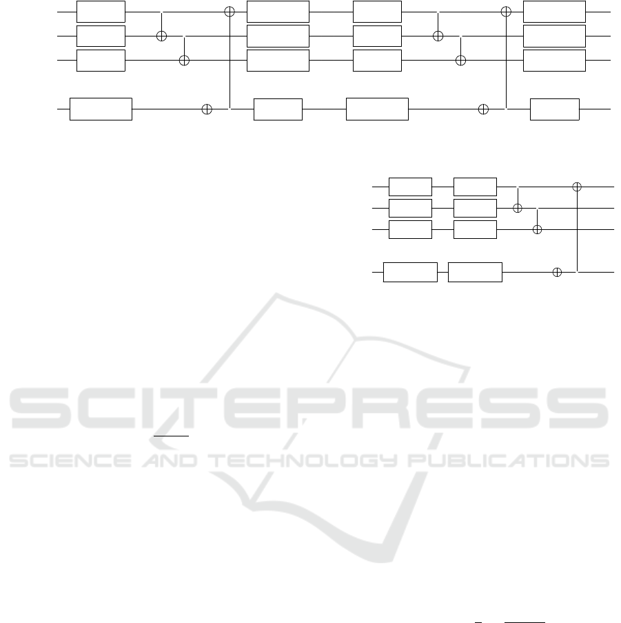
Entanglement, which is applied on QSVR

en=lin

re=0

Figure 5, can enhance the expressive power of quan-

tum feature maps, but it can also make the implemen-

tations of QSVMs more difﬁcult due to the increased

complexity of entangled quantum states. However,

another way of increasing the expressivity of a quan-

tum feature map is by the so-called data-reuploading

scheme (Schuld et al., 2021; Jerbi et al., 2023), which

is applied on QSVR

en=lin

re=1

in Figure 6 to make a more

expressive feature map. The entanglement layer,

which is implemented by a ring of CNOTs, is in be-

tween the encoding rotations due to the way quantum

kernel estimation is implemented (via the inversion

test) in some of our experiments.

3.5 Quantum Kernels

We use two types of quantum kernels in our exper-

iments: ﬁdelity and projected quantum kernels. We

use the inversion test for the quantum kernel estima-

tion of the ﬁdelity quantum kernels with the three fea-

ture maps introduced in section 3.4, whereas, for the

projected quantum kernels, we use the DensityMatrix

class from the Qiskit Quantum Information library.

Fidelity quantum kernels k(x

) via the inversion

test are given by

k(x

) =



⟨ψ(x

)|ψ(x

)⟩



, (5)

where ψ(x

) = U

)|0 . .. 0⟩ is the quantum state

after passing through the quantum feature map

φ(x

) applied on the i-th classical datapoint. We

ICAART 2024 - 16th International Conference on Agents and Artiﬁcial Intelligence

380

)

•

n−1

)

•

n−1

)

•

n−2

)

•

n−2

)

n−3

)

n−3

)

n−1

)

•

)

n−1

)

•

)

Figure 6: Quantum Feature Map for n features with entanglement and data re-uploading (below: QSVR

en=lin

re=1

rewrite Equation (5)

k(x

) =



⟨0.. .0|U

†

)|0 . .. 0⟩



⟨0.. .0|Φ

i j

⟩



(6)

where we deﬁned |Φ

i j

⟩ = U

†

)|0 . .. 0⟩.

Note that the term



⟨0.. .0|Φ

i j

⟩



is just the prob-

ability of measuring |Φ

i j

⟩ in the |0... 0⟩ state de-

noted by p

i j

(|0.. .0⟩). Hence, the ﬁdelity quan-

tum kernel is just the frequency of occurrences n

i j

of |Φ⟩ in the ground state

k(x

) = p

i j

(|0.. .0⟩) ,

i j

#shots

(7)

Using the quantum Hilbert space as the feature

space has the advantage that it grows exponen-

tially with the number of qubits used, which in

turn allows to obtain high-dimensional feature

maps. For instance, they are especially power-

ful for the creation of separating hyperplanes for

the classiﬁcation of astronomy data (Peters et al.,

2021). However, a feature map that is too high-

dimensional for a speciﬁc learning task might

be too expressive and fails. This is known as

the curse of dimensionality. For this reason, we

also use projected quantum kernels (Huang et al.,

2021) because they circumvent this issue by pro-

jecting back into the classical space.

Projected Quantum Kernels: k(x

) that we use

are given by

k(x

) = exp

−γ

∑

k=0



) −ρ

)



(8)

where γ > 0 and the reduced density matrix ρ

)

denotes the density matrix ρ(x

) created by the

quantum feature map applied on the datapoint x

) R

)

•

) R

)

•

) R

)

n−1

n−2

) R

n−1

)

•

Figure 7: Quantum Feature Map for n features with entan-

glement by CNOT gates (below: QSVR

proj

where all but the k-th qubit (of total n

) are traced

out. Note that it is sufﬁcient for this type of quan-

tum kernel to know only the reduced density ma-

trix - not the full density matrix. We obtain these

by calculating the full density matrix and evalu-

ating the reduced density matrices by taking the

partial traces from it.

3.6 Performance Metric

Within this work, we use the accuracy to benchmark

the performance of the introduced methods.

Accuracy: measures the predictive power of an ML

model. In the context of this work, the mean ab-

solute percentage error (MAPE)

MAPE =

∑

i=1

− ˆy

(9)

is used to calculate the performance, with y

be-

ing the true value, ˆy

the predicted value and n the

number of data points.

4 RESULTS

This section presents the results of the experiments.

All measurements were performed on a Ubuntu Linux

20.04.5 LTS system with 64 GB RAM and an AMD

Ryzen Threadripper 192X 12-Core Processor. We

used Qiskit (IBM-Qiskit, 2023; IBM, 2018) and

Evaluating Quantum Support Vector Regression Methods for Price Forecasting Applications

381

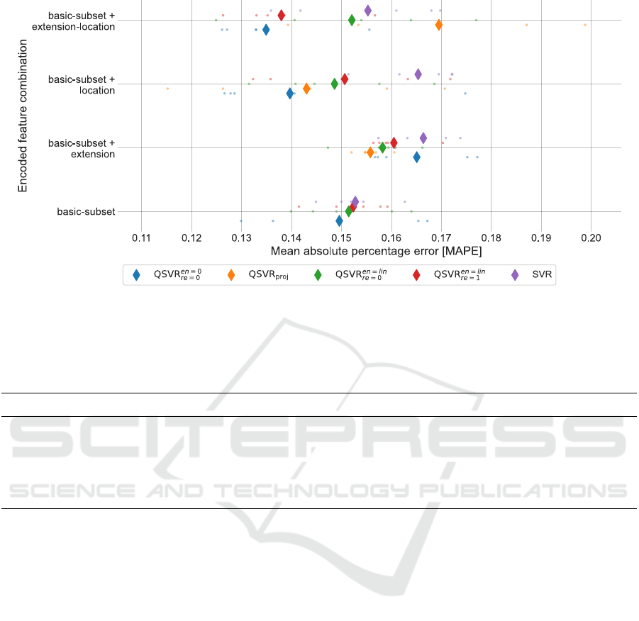
Figure 8: Accuracy for the encoded feature sets, in form of MAPE. Diamonds depict the average results over 5 repetitions.

Single measurements are displayed as dots. QSVR

proj

needs at least four features; therefore, there are no basic subset results

for QSVR

proj

Table 4: Overview of the MAPE for the encoded and unencoded datasets of the complete feature set. The best results are

highlighted in bold. * SVR and QSVR

proj

produce identical results for the unencoded, identical datasets.

Method Encoded datasets [MAPE] Unencoded datasets [MAPE]

SVR 0.1560±0.0133 0.1452 *

QSVR

en=0

re=0

0.1349±0.0110 0.1517±0.0025

QSVR

en=lin

re=0

0.1521±0.0181 0.1368±0.0079

QSVR

en=lin

re=1

0.1380±0.0102 0.1481±0.0076

QSVR

proj

0.1695±0.0216 0.1511 *

Qiskit Aer (Wood, 2019) for all QC simulations and

conducted ﬁve independent measurements with the

identical 80% / 20% holdout training/test split.

Accuracy

The accuracy, in terms of the MAPE, of the differ-

ent methods is depicted in Figure 8 for the encoded

datasets and in Figure 9 for the unencoded datasets. In

particular, these ﬁgures visualize the following char-

acteristics:

1 On the encoded datasets, all of the applied QSVR

methods, with the exception of QSVR

proj

for the

complete dataset, perform better than the classical

SVR implementation.

2 On the unencoded datasets, with the ex-

ception of the basic dataset, QSVR

en=lin

re=0

QSVR

proj

perform better than the classical SVR

method.

3 All results indicate good prediction qualities for

the encoded and unencoded datasets as they are

roughly within the interval [0.13, 0.17].

4 QSVR

en=0

re=0

performs best in three out of four en-

coded feature sets. It shows the overall best per-

formance for the encoded feature set but worst

in three out of four unencoded feature sets.

QSVR

en=lin

re=0

performs best for the unencoded fea-

ture sets. Examining these results in detail and the

impact of AE on the different QSVR methods will

be systematically analyzed in future work.

5 The encoded datasets exhibit much more variance

than the unencoded datasets. This is due to the

variance of the autoencoder. This exhibits the in-

ﬂuence of the AE on the accuracy of the results.

This fact needs to be taken into account for each

calculation.

6 The impact of the features is obvious for both un-

encoded and encoded datasets. Adding the ex-

tension features to the basic subset downgrades

the accuracy within the unencoded and encoded

datasets. The best result is always achieved within

ICAART 2024 - 16th International Conference on Agents and Artiﬁcial Intelligence

382

Figure 9: Accuracy for the unencoded feature sets, in form of MAPE. Diamonds depict the average results over 5 repetitions.

Single measurements are displayed as dots. QSVR

proj

needs at least four features; therefore, there are no basic subset results

for QSVR

proj

the complete feature set.

The MAPE values of all ﬁve methods for the complete

feature set of the encoded and unencoded data sets are

depicted in Table 4.

5 CONCLUSION

This work analyzed the potential of QMLs methods as

a substitution for linear, polynomial, or RBF kernels

for the SVR algorithm. In our case study, predicting

the residual value of used heavy construction equip-

ment, all simulated QML methods were shown to be

comparable or even better than the classical SVM

kernels regarding the MAPE scores. Therefore, we

showed that current state-of-the-art QSVR algorithms

are able to substitute the classical SVR implementa-

tions.

It has to be mentioned that we only examined a

limited number of QML methods on four variations of

a single data set, so general statements are therefore

limited by our choice of methods.

In order to strengthen the signiﬁcance of our

statistics, we will extend our survey to additional

and in particular open-source data sets. This analy-

sis will enable us to validate and substantially gen-

eralize the statements of our paper. Furthermore, we

will examine the role of entanglement and the power

of quantum kernels in more detail. We will analyze

the impact of dimensionality reduction, which will be

mandatory in the near future for datasets with larger

feature sets, on the quantum model performance in

future work. Finally, we will add more QML meth-

ods to our case study and integrate a real QC hard-

ware backend into our framework to be able to run

the QML algorithms on a real QC.

ACKNOWLEDGEMENTS

This work was partly funded by the German Federal

Ministry of Economic Affairs and Climate Action in

the research project AutoQML.

REFERENCES

Aaronson, S. and Gottesman, D. (2004). Improved sim-

ulation of stabilizer circuits. Physical Review A,

70(5):052328.

Alshboul, O., Shehadeh, A., Al-Kasasbeh, M., Al Mam-

look, R. E., Halalsheh, N., and Alkasasbeh, M. (2021).

Deep and machine learning approaches for forecasting

the residual value of heavy construction equipment:

a management decision support model. Engineering,

Construction and Architectural Management.

Bank, D., Koenigstein, N., and Giryes, R. (2020). Autoen-

coders. arXiv preprint arXiv:2003.05991.

Biamonte, J., Wittek, P., Pancotti, N., Rebentrost, P., Wiebe,

N., and Lloyd, S. (2017). Quantum machine learning.

Nature, 549(7671):195–202.

Cavallaro, G., Willsch, D., Willsch, M., Michielsen, K.,

and Riedel, M. (2020). Approaching remote sensing

Evaluating Quantum Support Vector Regression Methods for Price Forecasting Applications

383

image classiﬁcation with ensembles of support vector

machines on the d-wave quantum annealer. In IGARSS

2020-2020 IEEE International Geoscience and Re-

mote Sensing Symposium, pages 1973–1976. IEEE.

Chiteri, M. (2018). Cash-ﬂow and residual value analysis

for construction equipment. Master’s thesis, Univer-

sity of Alberta.

Cortes, C. and Vapnik, V. (1995). Support-vector networks.

Machine learning, 20:273–297.

Das, A. and Chakrabarti, B. K. (2005). Quantum anneal-

ing and related optimization methods, volume 679.

Springer Science & Business Media.

Géron, A. (2022). Hands-on machine learning with Scikit-

Learn, Keras, and TensorFlow. " O’Reilly Media".

Grossi, M., Ibrahim, N., Radescu, V., Loredo, R., Voigt, K.,

von Altrock, C., and Rudnik, A. (2022). Mixed quan-

tum–classical method for fraud detection with quan-

tum feature selection. IEEE Transactions on Quantum

Engineering, 3:1–12.

Harrow, A. W., Hassidim, A., and Lloyd, S. (2009). Quan-

tum algorithm for linear systems of equations. Physi-

cal review letters, 103(15):150502.

Hauke, P., Katzgraber, H. G., Lechner, W., Nishimori, H.,

and Oliver, W. D. (2020). Perspectives of quantum

annealing: Methods and implementations. Reports on

Progress in Physics, 83(5):054401.

Havlí

cek, V., Córcoles, A. D., Temme, K., Harrow, A. W.,

Kandala, A., Chow, J. M., and Gambetta, J. M. (2019).

Supervised learning with quantum-enhanced feature

spaces. Nature, 567(7747):209–212.

Huang et al., H.-Y. (2021). Power of data in quantum ma-

chine learning. Nature Communications, 12(1):2631.

IBM (2018). An open high-performance simulator for

quantum circuits. IBM Research Editorial Staff.

IBM-Qiskit (2023). Qiskit github page. https://github.com/

Qiskit.

Jerbi, S., Fiderer, L. J., Nautrup, H. P., Kübler, J. M.,

Briegel, H. J., and Dunjko, V. (2023). Quantum ma-

chine learning beyond kernel methods. Nature Com-

munications, 14(1).

Kadowaki, T. and Nishimori, H. (1998). Quantum anneal-

ing in the transverse ising model. Physical Review E,

58(5):5355.

Liu, Y., Arunachalam, S., and Temme, K. (2021). A rig-

orous and robust quantum speed-up in supervised ma-

chine learning. Nature Physics, 17(9):1013–1017.

Lucko, G., Vorster, M. C., and Anderson-Cook, C. M.

(2007). Unknown element of owning costs - impact

of residual value. JCEMD4, 133(1).

Miloševi

c, I., Kova

cevi

c, M., and Petronijevi

c, P. (2021).

Estimating residual value of heavy construction equip-

ment using ensemble learning. JCEMD4, 147(7).

Newman, D. A. (2014). Missing data: Five practical guide-

lines. Organizational Research Methods, 17(4).

Ng, A. et al. (2011). Sparse autoencoder. CS294A Lecture

notes, 72(2011):1–19.

Peters et al., E. (2021). Machine learning of high dimen-

sional data on a noisy quantum processor. npj Quan-

tum Information, 7(1):161.

Schölkopf, B., Smola, A. J., Bach, F., et al. (2002). Learn-

ing with kernels: support vector machines, regular-

ization, optimization, and beyond. MIT press.

Schuld, M., Fingerhuth, M., and Petruccione, F. (2017).

Implementing a distance-based classiﬁer with a

quantum interference circuit. Europhysics Letters,

119(6):60002.

Schuld, M., Sweke, R., and Meyer, J. J. (2021). Effect of

data encoding on the expressive power of variational

quantum-machine-learning models. Physical Review

A, 103(3):032430.

Shehadeh, A., Alshboul, O., Al Mamlook, R. E., and Hame-

dat, O. (2021). Machine learning models for predict-

ing the residual value of heavy construction equip-

ment: An evaluation of modiﬁed decision tree, light-

gbm, and xgboost regression. Automation in Con-

struction, 129:103827.

Shor, P. W. (1999). Polynomial-time algorithms for prime

factorization and discrete logarithms on a quantum

computer. SIAM review, 41(2):303–332.

Steinwart, I. and Christmann, A. (2008). Support vector

machines. Springer Science & Business Media.

Stühler., H., Zöller., M., Klau., D., Beiderwellen-

Bedrikow., A., and Tutschku., C. (2023). Benchmark-

ing automated machine learning methods for price

forecasting applications. In Proceedings of the 12th

International Conference on Data Science, Technol-

ogy and Applications - DATA, pages 30–39. INSTICC,

SciTePress.

Thanasilp, S., Wang, S., Cerezo, M., and Holmes, Z.

(2022). Exponential concentration and untrainabil-

ity in quantum kernel methods. arXiv preprint

arXiv:2208.11060.

Tschannen, M., Bachem, O., and Lucic, M. (2018). Recent

advances in autoencoder-based representation learn-

ing. arXiv preprint arXiv:1812.05069.

Vapnik, V. N. (1999). An overview of statistical learn-

ing theory. IEEE transactions on neural networks,

10(5):988–999.

Willsch, D., Willsch, M., De Raedt, H., and Michielsen,

K. (2020). Support vector machines on the d-wave

quantum annealer. Computer physics communica-

tions, 248:107006.

Wood, C. J. (2019). Introducing qiskit aer: A high per-

formance simulator framework for quantum circuits.

Medium.

Wo´zniak, K. A., Belis, V., Puljak, E., Barkoutsos, P., Disser-

tori, G., Grossi, M., Pierini, M., Reiter, F., Tavernelli,

I., and Vallecorsa, S. (2023). Quantum anomaly de-

tection in the latent space of proton collision events at

the lhc. arXiv preprint arXiv:2301.10780.

Zöller, M.-A., Nguyen, T.-D., and Huber, M. F. (2021).

Incremental search space construction for machine

learning pipeline synthesis. In Advances in Intelligent

Data Analysis XIX.

Zong, Y. (2017). Maintenance cost and residual value pre-

diction of heavy construction equipment. Master’s

thesis, University of Alberta.

Zoph, B. and Le, Q. V. (2016). Neural architecture

search with reinforcement learning. arXiv preprint

arXiv:1611.01578.

ICAART 2024 - 16th International Conference on Agents and Artiﬁcial Intelligence

384