Military Badge Detection and Classiﬁcation Algorithm for Automatic

Processing of Documents

Charith Gunasekara

1 a

, Yash Matharu

2 b

and Rohan Ben Joseph

3 c

Department of National Defence, Government of Canada, Ottawa, ON, Canada

Faculty of Engineering, McMaster University, Hamilton, ON, Canada

Department of Computing Science, Simon Fraser University, Burnaby, BC, Canada

Keywords:

Computer Vision, Object Detection, Document Classiﬁcation, YOLOv5.

Abstract:

This paper outlines a robust approach to automate the detection of military badges on ofﬁcial government

documents utilizing YOLOv5 computer vision model. In an era where the rapid classiﬁcation and management

of sensitive documents is paramount, developing a system capable of accurately identifying and classifying

distinct badge types plays a crucial role in supporting data management and security protocols. To address

the challenges posed by the lack of accessible, real-world government and military documents for research,

we introduced a novel method to simulate training data. We employ a technique that automates the data

labelling process, facilitating the generation of a comprehensive and versatile dataset while eliminating the

risk of compromising sensitive information. Through careful model training and hyper-parameter tuning, the

YOLOv5 model demonstrated exemplary performance, successfully detecting a wide spectrum of badge types

across various documents.

1 INTRODUCTION

The sheer volume of documents generated presents

a unique challenge in large-scale organizations such

as governmental departments and the military. Tradi-

tional manual methods of document classiﬁcation are

not only labour-intensive but also time-consuming. In

the pursuit of efﬁciency, there’s a growing trend to-

wards automation. However, this path isn’t devoid of

challenges. For one, access to open data for research

is restricted, often due to strict organizational security

policies. This limits the potential to utilize vast inter-

nal datasets for training sophisticated machine learn-

ing models (Brown, 2010). Such constraints are in-

deed a missed opportunity, especially when machine

learning algorithms have showcased proﬁciency in

tasks demanding domain knowledge and uncompro-

mising attention (Orosz et al., 2022).

The appeal of document classiﬁcation through

machine learning is evident, yet earlier attempts in

this direction often stumbled due to data scarcity and

the tedious nature of data labelling (Song et al., 2019)

https://orcid.org/0000-0002-7213-883X

https://orcid.org/0009-0003-8635-4239

https://orcid.org/0000-0001-8069-5874

(Ciecierski and Kamola, 2020) (Huber-ﬂiﬂet et al.,

2019). In a novel approach, (Chiu et al., 2010) lever-

aged Optical Character Recognition (OCR) for ex-

tracting textual content and employed the Normalized

Cuts algorithm for clustering non-textual pixels. Al-

though innovative, this methodology was heavily re-

liant on manually labelled data, reducing its scalabil-

ity.

A unique approach was introduced by (Kallem-

pudi et al., 2022), who proposed the ”Soft Teacher”

mechanism. This semi-supervised pipeline catered

to graphical object detection within scanned docu-

ment images, even when working with limited la-

belled data. Similarly, (Arvind, 2023) integrated OCR

for keyword vector selection in classifying govern-

ment documents. Yet, their endeavours were limited

by training data, a recurring issue predominantly due

to access restrictions. Delving deeper into automating

document feature recognition, (Forczma

nski et al.,

2020) showcased a technique that employed Convolu-

tional Neural Networks (CNN) to automatically seg-

ment various elements, such as logos, stamps, and

text blocks, from paper documents. Their CNN-

centric approach was validated as superior when com-

pared with the conventional cascade-based detection

method.

Gunasekara, C., Matharu, Y. and Ben Joseph, R.

Military Badge Detection and Classiﬁcation Algorithm for Automatic Processing of Documents.

DOI: 10.5220/0012351300003654

Paper copyright by his Majesty the King in Right of Canada as represented by the Minister of National Defence

In Proceedings of the 13th International Conference on Pattern Recognition Applications and Methods (ICPRAM 2024), pages 723-731

ISBN: 978-989-758-684-2; ISSN: 2184-4313

723

A signiﬁcant paradigm shift in the realm of ob-

ject detection was heralded by the birth of the You

Only Look Once (YOLO) algorithm (Redmon et al.,

2016). YOLO, and its subsequent iterations showed

the ﬁrst one-stage detection mechanism in the deep

learning, outclassing many existing algorithms in ac-

curacy and speed (Zou et al., 2023). Though alter-

native one-stage object detection models like RestNet

have been explored, especially for tasks like logo de-

tection (Sarwo et al., 2019), YOLO is still leading in

terms of efﬁciency (Deng et al., 2023). Building on

YOLO’s foundation, (Bailey et al., 2022) crafted a

training dataset for bounding boxes tailored for var-

ied object detection. Meanwhile, (Rezkiani et al.,

2022) employed YOLOv4 to discern logos on uni-

versity diplomas, aiming for document classiﬁcation.

However, the prevailing challenge remains the man-

ual labelling of objects and bounding boxes, which

inevitably makes the entire process labour-intensive.

Several versions of YOLO have been introduced since

its inception. Table 1 showcases the popularity of

each version through their respective Github stars.

While the newer version YOLOv8’s real advantage

comes in applications that require real-time object de-

tection, YOLOv5 is preferred for still object detection

primarily due to its robust Pytorch-based ecosystem

and extensive documentation support.

While advancements have been made in object de-

tection and document classiﬁcation, a real gap ex-

ists regarding specialized domains like military and

governmental sectors. The lack of publicly available

data due to organizational security policies and man-

ual labour involved in creating training datasets in the

labelling and marking bounding boxes severely throt-

tles the speed and efﬁciency of the model training pro-

cess. When considering the volume of ofﬁcial doc-

uments generated daily, this poses a signiﬁcant bot-

tleneck. We introduce an algorithm capable of au-

tonomously creating training datasets, eliminating the

requirement for manual labelling of data. By em-

ploying data augmentation techniques, our algorithm

generates synthetic dataset to replicate the features

and complexities of real-life scanned sensitive doc-

uments. This not only avoids labour-intensive manual

labelling but also paves the way for scalable and efﬁ-

cient document classiﬁcation in this domain.

2 RESEARCH METHODOLOGY

2.1 Data Collection

The overarching objective of this research is to

classify Canadian military documents based on the

Table 1: GitHub Popularity of YOLO Versions.

YOLO Version GitHub Stars in 1000s

YOLO v3 9.7

YOLO v4 21

YOLO v5 41.9

YOLO v6 5.2

YOLO v7 11.3

YOLO v8 13.2

badges imprinted on them. To achieve this, a com-

prehensive dataset was required to train our model ef-

ﬁciently. Utilizing existing documents with badges

for this purpose was not deemed practical due to two

primary concerns:

a) Training an image detection model effectively

mandates thousands of training samples for each

class. Manual labelling of such vast quantities of data

proves to be labour-intensive and time-consuming. b)

The pre-existing documents house sensitive informa-

tion, making them unsuitable for open research.

Given these limitations, the decision was made to

develop a mock dataset mirroring the patterns found

in these military documents. The process for con-

structing this mock dataset is detailed below:

1. Badge Compilation. An exhaustive collection was

undertaken of badges from various Canadian mili-

tary organizations to serve as our primary dataset.

2. Document Template Collection. We procured in-

ternal document templates and unﬁlled forms, en-

suring that they do not contain any sensitive infor-

mation. This provided us with the base structure

over which badges could be overlaid.

3. Mock Document Creation. A simulated set of

labelled documents was constructed using the

gathered badges and document templates. The

methodology adopted for pasting the badges onto

the documents involves a data augmentation algo-

rithm, elaborated in the subsequent section.

The abovementioned approach ensured the synthesis

of a robust dataset, eliminating risks associated with

using genuine documents and signiﬁcantly reducing

manual labelling efforts. This mock dataset, we be-

lieve, will sufﬁciently represent the sophistication of

real-world military documents, aiding in the effective

training of our image detection model.

2.2 Data Pre-Processing and

Augmentation

In order to provide an effective training ground for

the YOLO5 model, we undertook extensive data pre-

processing and augmentation measures. Our dataset

combined both the badge and document datasets to

ICPRAM 2024 - 13th International Conference on Pattern Recognition Applications and Methods

724

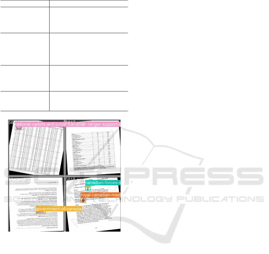
Table 2: Badge and Logo Data Sources and URLs.

Data Source URL

Gallery of Cana-

dian Force Badges

https://www.canada.ca/en/

services/defence/caf/military-

identity-system/canadian-

forces-badges.html

Government of

Canada Logo

https://www.international.gc.ca/

world-monde/assets/images/

funding-ﬁnancement/canada-

aid-aide/canada-wordmark-

colour.jpg

National Defence

Logo

https://media.socastsrm.com/

wordpress/wp-content/

blogs.dir/1977/ﬁles/2021/05/

national-defence.png

DRDC Logo https://www.canada.ca/content/

dam/drdc-rddc/images/articles/

2021/drdc-logo.jpg

Figure 1: Sample dataset of generated images.

create an encompassing platform for model training.

Adhering to best practices as suggested by the YOLO

V5 model’s library, we established a target of at least

1,100 images per class. This culminated in a training

dataset with 55,400 labelled objects per class and a

subsequent validation set comprising 13,860 images

distributed evenly across all badge and logo classes.

We ensured the inclusion of images depicting var-

ied environmental conditions – from assorted lighting

scenarios to differing viewing angles and diverse im-

age sources like online scrapes, local collections, and

captures from various camera types.

To effectively train the model to adapt to real-

world conditions, each image underwent rigorous

processing:

1. Image Resizing. All images were resized to 640 x

640 pixels, the default resolution supported by the

YOLOv5 model.

2. Basic Augmentations. These included random

horizontal and vertical ﬂips with a 50% probabil-

ity, along with random rotations in the range of

-15 to 15 degrees.

3. Badge Integration and Augmentation. Randomly

selected documents were resized to the default

YOLO V5 resolution. Then, anywhere from 0 to

10 badges were randomly selected and underwent

the aforementioned augmentations. Badge sizes

were varied (60 to 125 pixels width), with heights

adjusted to keep aspect ratios intact. Badge place-

ment was randomized within set coordinate limits,

ensuring varied placement within the document,

thereby exposing the model to a plethora of sizes

and placements.

4. Global Augmentations. The application of global

augmentations plays a crucial role in training

models, particularly in creating scenarios that

mimic real-world conditions. One common ap-

proach to enhance the robustness of a model is to

introduce Gaussian noise during the data augmen-

tation stage. This method helps in simulating vari-

ations and imperfections in real-world data. Dur-

ing the selection of augmentations, a balance be-

tween noise and accuracy was a critical consider-

ation.

Moderate introduction of Gaussian noise can

serve to regularize the model during training,

thereby improving its generalization capabilities.

It allows the model to become resilient to noise

and slight variations in the input data, poten-

tially reducing overﬁtting and enhancing accuracy

when evaluating the model with real-world im-

ages that naturally contain some noise. On the

contrary, a high level of Gaussian noise might de-

grade the model’s performance, making it difﬁcult

for the model to learn meaningful patterns from

the data and possibly leading to increased error

rates.

• Gaussian Noise. Gaussian noise, with a sigma

(standard deviation) value of 0.5, was intro-

duced to mimic the common noise encountered

during the scanning of documents. A sigma

value of 0.5 was chosen to balance the introduc-

tion of noise for robustness while maintaining

the accuracy of object detection in the YOLO

model. This moderate level of noise ensures

that while the data contains variations, it does

not become unrecognizable. Thus, images with

moderate noise maintain semantic similarity to

the original, allowing the model to learn robust

features while managing real-world variations

Military Badge Detection and Classiﬁcation Algorithm for Automatic Processing of Documents

725

(Liu et al., 2018),(Li and Ghosal, 2014).

• Gaussian Blur. Gaussian Blur was also utilized

to account for potential losses in detail or soft-

ening of edges that can occur during scanning.

That was implemented with a sigma value rang-

ing from 0.1 to 1 and used a kernel size of (3,

3). This approach ensures that the model can

adapt to potential variations in image sharp-

ness, thereby enhancing its performance with

varying image qualities (Suto, 2023). In Gaus-

sian blurring, the kernel size inﬂuences the ex-

tent of smoothing applied to the image, mak-

ing it an essential hyperparameter for tailoring

image processing tasks, balancing the ability of

the model to learn to interpret noisy and blurred

images against the preservation of important

features for the feature detectors to detect pat-

terns from hierarchically. The kernel size of (3,

3) in Gaussian blur operations signiﬁes a rela-

tively small kernel, resulting in localized blur-

ring and preserving ﬁner details in the image. It

denotes a 3x3 grid used for convolution, where

each pixel’s value is recalculated as an aver-

age of the neighbouring nine pixels, giving a

smoothing effect.

Maintaining consistency and accuracy in labelling

is crucial. Every image’s labelling was ensured to

be thorough and accurate, as partial labelling ham-

pers effective training. Background images without

objects were also incorporated into the dataset (repre-

senting 0-10% of the total) to reduce false positives.

Each processed image was saved in PNG (Portable

Network Graphics) format, signifying the culmina-

tion of both document and badge integration. Along-

side, a text ﬁle was generated to serve the YOLO

model, detailing badge locations in the format:

class_number, x_center, y_center, width, height

All coordinate values were adjusted to the image’s

dimensions for normalization purposes by dividing by

the 640-pixel width or height.

The program used for the dataset generation pro-

cess is explained in Algorithm 1.

2.3 Model Training

The essence of achieving optimal performance in

deep learning applications lies in the careful selection

and ﬁne-tuning of hyperparameters, determining how

a model learns and adapts to given data. Our focus in

this section is to elucidate the training process for our

chosen YOLOv5 model.

Given our dataset’s size, we deemed it advanta-

geous to initiate our training using the pre-trained

Data: Total number of pages, dataset name

Result: Pages and text ﬁles saved to output

directory

initialization, Create maps for class number

to badge, and document number to

document ﬁlename;

for each page created do

Select random number of badges;

Select random document;

Load in document, resize to 640x640 and

augment by horizontally/vertically

ﬂipping, and rotating;

Open a text ﬁlet;

for each badge do

Load in badge and augment by

horizontally/vertically ﬂipping and

rotating;

Paste badge onto document;

Write to txt ﬁle class and coordinates;

end

Augment combined document + badge

page using gaussian noise and blur Save

page as PNG ﬁle

end

Algorithm 1: Algorithm for generating the dataset.

weights from YOLOv5’s default set. Such a decision

often aids in faster convergence, especially when data

volume is limited.

2.3.1 Hyper-Parameters

The summary of our chosen hyper-parameters and

their respective roles in the training process is given

below.

• Learning Rate. Our experiments were done us-

ing a learning rate of 0.02. The signiﬁcance of this

hyper-parameter lies in the step size for updating

model parameters. Careful tuning is imperative to

avoid rapid divergence or protracted convergence.

• Batch Size. Ensuring efﬁcient computation while

retaining model generalization, our batch size was

set at 16. This balances between computational

needs and the potential beneﬁts of more frequent

model updates.

• Epochs. The number of epochs for the training

cycles was set to 55 to allow enough time for the

model to converge the loss functions to a mini-

mum value. At the same time, we monitored the

model performance with a validation set to ensure

it does not overﬁt.

• Optimizer Selection. Our model was trained us-

ing the Stochastic Gradient Descent (SGD) opti-

mizer, chosen for its synergy with Pytorch. SGD

ICPRAM 2024 - 13th International Conference on Pattern Recognition Applications and Methods

726

is an iterative process where, at each step, a

subset of the training data (mini-batch) is used

to compute gradients and update model param-

eters. Accompanying hyperparameters, such as

momentum (set at 0.937) and weight decay (set at

0.0005), were carefully selected to inﬂuence the

optimizer’s behaviour, ensuring efﬁcient conver-

gence.

• Architectural Regularizations. The dropout

rate, ﬁxed at 0.5, ensured periodic deactivation of

neurons, enabling model robustness. Meanwhile,

batch normalization, with momentum set at 0.937,

contributed to training stability.

2.4 Training Environment

The model training was conducted on multiple GPUs

on a cloud-based virtual machine (VM) with the fol-

lowing speciﬁcations:

• RAM (Random Access Memory): 224GB

• CPUs (Central Processing Units): 12 virtual

CPUs (vCPUs)

• Generation: V2

• Architecture: 64-bit (x64)

• Operating System: Linux

• VRAM (Video RAM) per GPU (Graphics Pro-

cessing Units) : 24GB

• Number of GPUs: 2

• Temp storage (SSD(Solid State Drives)): 1474GB

• GPU memory: 32GB

• Max data disks: 24

• Max uncached disk throughput: 40000/400

(IOPS(Input/Output Operations Per Sec-

ond)/MBps(Megabytes Per Second))

• Max NICs (Network Interface Cards): 8

3 RESULTS

While training our models, we evaluated the model’s

performance on a separate validation dataset, which

comprised document objects unfamiliar to the models

from their training phase. The subsequent subsections

provide an in-depth analysis of the performance met-

rics obtained from this testing process.

3.1 Precision and Recall

Precision and recall are crucial indicators of a ma-

chine learning model’s performance in classiﬁcation

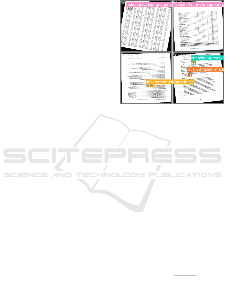
Figure 2: Sample dataset of predicted images.

tasks. While precision (Equation 1) gives us an in-

sight into the correctness of our model by measuring

the ratio of true positive (TP) predictions to the sum

of true positive (TP) and false positive (FP) predic-

tions, recall (Equation 2) on the other hand, highlights

the model’s ability to identify all relevant instances by

evaluating the ratio of true positive(TP) predictions to

the sum of true positive (TP) and false negative (FN)

predictions.

Through the graphical representations depicted in

Figure 3 for Precision vs. Epochs and Figure 4 for

Recall vs. Epochs, we can draw some insightful con-

clusions about the model’s behaviour over training

epochs. As seen in Figure 3, the precision values are

rising as the training epochs increase. Remarkably,

after the 10th epoch, the precision converges to an im-

pressive 99.5%. This connotes that our model, by this

stage, has honed its ability to predict true positives

with negligible false positive rates.

On the other hand, the recall values, as shown in

Figure 4, do demonstrate improvement as the training

progresses by converging to a score of 99.78%. This

suggests that while the model has become adept at

correctly classifying the positive cases, it still misses

out on some, leading to a higher number of false neg-

atives as compared to false positives.

Precision =

T P

(T P + FP)

(1)

Recall =

T P

(T P + FN)

(2)

Military Badge Detection and Classiﬁcation Algorithm for Automatic Processing of Documents

727

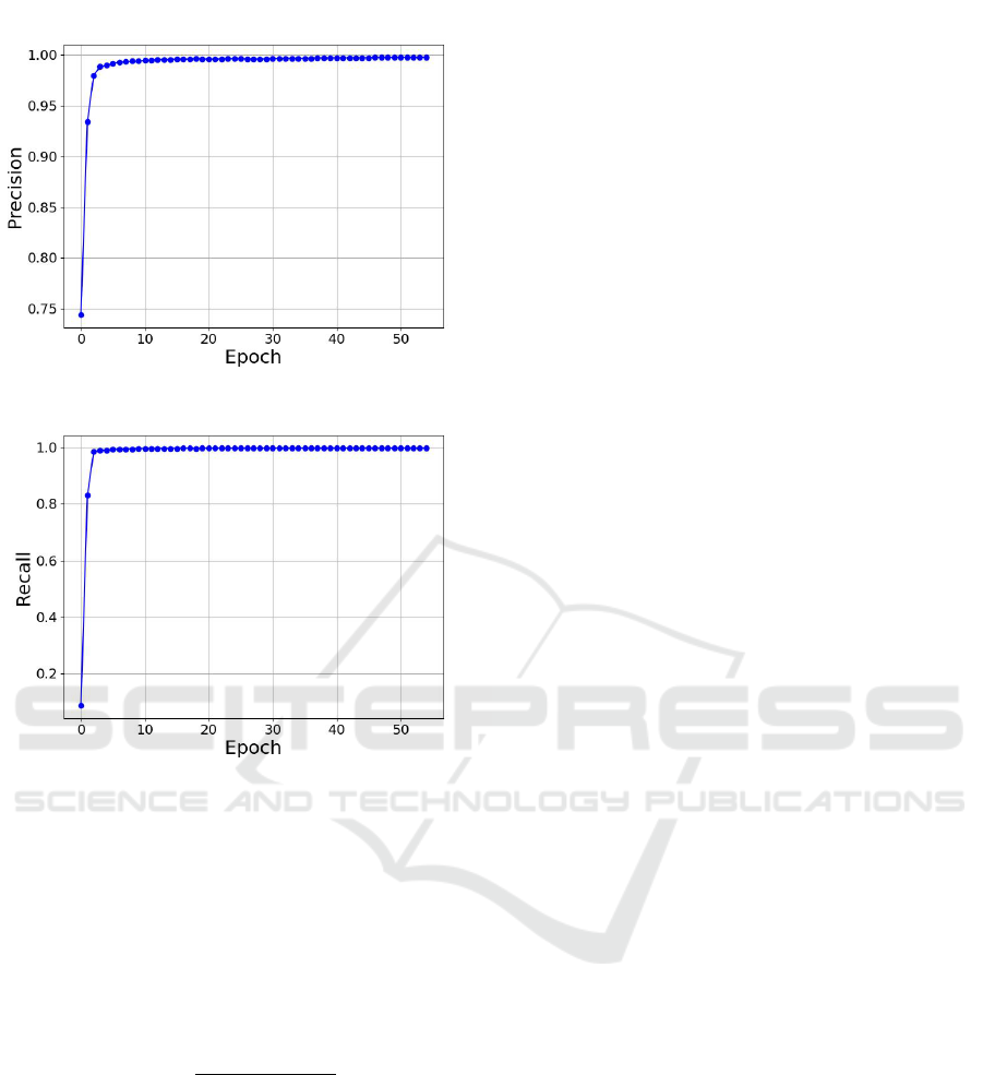
Figure 3: Precision vs Epochs Curve.

Figure 4: Recall vs Epochs Curve.

3.2 Intersection over Union (IoU)

Intersection over Union (IoU) The Intersection over

Union (IoU) provides a quantitative assessment of the

precision of predicted bounding boxes by measuring

their overlap with respective ground truth boxes. IoU

is obtained by computing the ratio of the area of in-

tersection to the area of union between the predicted

and true boxes.

IoU =

Area of Overlap

Area of Union

(3)

IoU values span from 0, representing no overlap, to 1,

indicative of a perfect match between the predicted

and actual bounding boxes. Employing IoU as a

threshold metric, accurate predictions are acknowl-

edged when the IoU surpasses a predetermined value.

As elaborated in section 3.3, the performance of

the model is evaluated using a threshold of 0.5, ensur-

ing at least 50% overlap of the predicted box with the

ground truth, and a spectrum of IoU thresholds from

0.5 to 0.95, inclusive of several intermediate values.

The average precision is calculated distinctly for each

threshold, followed by the computation of the mean.

The mAP 0.5:0.95 furnishes a holistic evaluation of

the model’s performance, encapsulating its efﬁcacy

across many overlap scenarios. This is perceived as

a rigorous evaluation metric due to its imperative for

high accuracy across diverse IoU levels.

3.3 Mean Average Precision (mAP)

In object detection and classiﬁcation, Mean Aver-

age Precision (mAP) is a vital metric aggregating

the model’s performance across different conﬁdence

thresholds. It combines precision and recall effec-

tively, providing a holistic view of the model’s abil-

ity to identify objects and minimize false detections

correctly. The mAP score is calculated by taking the

average of the Average Precision (AP) values for each

class or category of objects. AP, in turn, is determined

by plotting the precision-recall curve for a speciﬁc

class and calculating the area under that curve. (Hen-

derson and Ferrari, 2017)

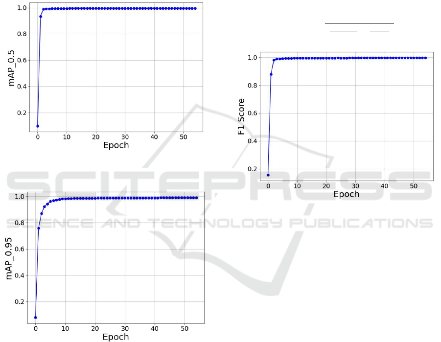
To better visualize our model’s performance

throughout training, we present the mAP curves in

Figures 5 and 6, illustrating how mAP values evolve

across training epochs. This graphical representation

aids in understanding the consistency and reliability

of our model in detecting document objects through-

out its training process.

The mAP’s progression over training epochs is

a strong indicator of the model’s learning trajectory.

a rising curve denotes a consistent enhancement in

object detection capabilities during the training pro-

cess. A mAP value inching closer to 1 indicates a

commendable performance, where the model adeptly

identiﬁes badge regions while effectively managing

false positives and false negatives.

Mean Average Precision at Intersection over

Union 0.5 (mAP 0.5) (Figures 5 ): This metric pro-

vides an assessment of average precision, stipulating

that predictions are deemed accurate when their In-

tersection over Union (IoU) with the corresponding

ground truth bounding boxes is 0.5 or above. Es-

sentially, it gauges the model’s proﬁciency in object

detection where there is a moderate overlap with the

ground truth annotations.

Mean Average Precision at Intersection over

Union 0.5:0.95 (mAP 0.5:0.95) (Figure 6): This eval-

uative metric expands the assessment to encompass an

array of IoU thresholds, speciﬁcally from 0.5 to 0.95,

including intermediate values. It independently deter-

mines the average precision for each threshold, sub-

sequently computing the mean of these values. The

mAP 0.5:0.95 thoroughly appraises the model’s ca-

pabilities, considering its performance across an ex-

tensive range of overlap scenarios. This metric is

ICPRAM 2024 - 13th International Conference on Pattern Recognition Applications and Methods

728

often viewed as a more rigorous evaluative gauge,

which mandates elevated precision across assorted

IoU levels. Both mAP 0.5 and mAP 0.5:0.95 serve

as instrumental metrics in applied settings. The mAP

0.5, affords insights into the model’s performance un-

der relatively forgiving conditions. In contrast, mAP

0.5:0.95 provides a more rigorous assessment, en-

suring the model sustains high precision, even when

object boundaries are meticulously aligned with the

ground truth annotations.

Figure 5: Mean Average Precision Curve over an IoU

threshold of 0.5.

Figure 6: Mean Average Precision Curve over an IoU

threshold range of 0.5 to 0.95.

3.4 F1 Scores

The F1 score, depicted in Equation 4, offers a com-

bined evaluation of a model’s precision and recall.

This metric becomes particularly insightful when

classes are distributed unevenly or when the impli-

cations of false positives differ markedly from false

negatives. Conceptually, the F1 score encapsulates

the overlap between a model’s predictions and the

ground truth. As visualized in Figure 7, we trace the

trajectory of the model’s F1 score across 55 epochs.

By calculating it as the harmonic mean between pre-

cision and recall, the F1 score is a comprehensive

metric, effectively harmonizing the balance between

these pivotal performance indicators. As the F1 score

converges to one, the model’s predictions increas-

ingly align with the actual data, showcasing optimal

precision and recall. This convergence to one indi-

cates near-perfect harmony between detected and ac-

tual document objects, reﬂecting the model’s exem-

plary performance.

F1 Score =

(

Precision

Recall

)

(4)

Figure 7: F1score vs Epochs Curve.

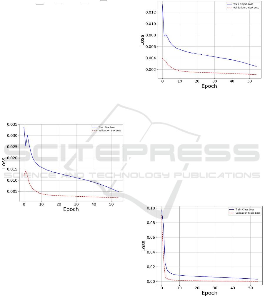
3.5 Loss Functions

Loss functions are used to quantify the difference be-

tween predicted values (output of a model) and ac-

tual target values (ground truth) during training. The

three primary loss components are box loss (minimiz-

ing discrepancies in predicted bounding box coordi-

nates), object loss (ensuring accurate object presence

prediction), and classiﬁcation loss (optimizing object

categorization accuracy). These loss functions work

together to guide the training process of our object de-

tection model, striving for improved accuracy in ob-

ject localization, object classiﬁcation, and the distinc-

tion between objects and background regions.

3.5.1 Box Loss

The box loss, as deﬁned in Equation 5 is the differ-

ence between the predicted bounding box parameters

(like center coordinates, width, and height) and the

actual ground truth parameters of the boxes. The ob-

jective of minimizing box loss is to improve the pre-

cision of the model in localizing objects within an im-

age.

Military Badge Detection and Classiﬁcation Algorithm for Automatic Processing of Documents

729

Box Loss =

∑

i=0

∑

j=0

obj

(k)

i j

[(x

i j

− ˆx

i j

)

+ (y

i j

− ˆy

i j

)

(

√

i j

−

ˆw

i j

)

+ (

i j

−

i j

)

] (5)

Here, (x

i j

, y

i j

) and (ˆx

i j

, ˆy

i j

) are the predicted

and true bounding box center coordinates, while

i j

, h

i j

) and ( ˆw

i j

are the predicted and true

bounding box width and height respectively. S

represents the number of grid cells, in S ×S grid and

B is the number of bounding boxes predicted per grid

cell, ob j

(k)

i j

is the boolean indicator of whether object

k exists in grid cell (i, j).

Depicted by the blue curve in Figure 8, the train-

ing box loss offers insights into the box loss trajec-

tory during the model’s learning phase. An evident

reduction in both training box loss and validation box

loss as epochs progress denotes the model’s sharpen-

ing ability in bounding box predictions throughout its

training epoch cycles.

Figure 8: Box Loss Curves.

3.5.2 Object Loss

Object Loss as shown in Equation 6 is computed us-

ing the mean squared error (MSE) between the pre-

dicted conﬁdence scores and the ground truth conﬁ-

dence scores where the conﬁdence scores conﬁdence

score indicates whether an object is present in a given

grid cell and how accurate the bounding box is.

Obj Loss =

∑

i=0

∑

j=0

ob j

(k)

i j

·(Con f

i j

−

Con f

i j

)

(6)

Here, Con f

i j

is the predicted conﬁdence score, and

Conf

i j

is the true conﬁdence score.

Figure 9 illustrates a concurrent decline in both

training and validation object loss as training pro-

gresses, indicating an enhancement in the model’s de-

tection capabilities. The absence of a signiﬁcant devi-

ation between these two metrics throughout the train-

ing epochs reassuringly suggests that the model is not

afﬂicted by issues such as over-ﬁtting.

Figure 9: Object Loss Curves.

3.5.3 Classiﬁcation Loss

The classiﬁcation loss is deﬁned as the misalignment

between the predicted class probabilities and the ac-

tual binary class labels within the training dataset,

measuring the model’s reliability in associating ob-

jects with their true categories. As visualized in Fig-

ure 10, an analogous declining trend observed in both

training and validation classiﬁcation loss across the

training epochs not only corroborates the model’s im-

proving proﬁciency in object classiﬁcation but also

mirrors the previously discussed trends in box and ob-

ject loss, solidifying the consistency in the model’s

learning and adaptation throughout the training pro-

cess.

Figure 10: Classiﬁcation Loss Curves.

ICPRAM 2024 - 13th International Conference on Pattern Recognition Applications and Methods

730

4 CONCLUSION

In conclusion, this paper introduced a well-rounded

approach toward automated military badge detection

on government documents by utilizing the YOLOv5

model. By innovatively automating the training data

labelling process and generating a simulated dataset

of military and ofﬁcial documents, circumventing the

issue of public unavailability, a scalable and precise

badge detection system was established. Through

strategic training and hyper-parameter tuning, the

YOLOv5 model showcased substantial proﬁciency in

detecting various badge types within the documents,

illustrating a promising stride in document-based ob-

ject detection.

REFERENCES

Arvind, N. (2023). A semi-automatic method for document

classiﬁcation in the shipping industry. In Proceedings

of Neptune’s conference, Samudramanthan 2023 IIT

Kharagpur.

Bailey, E. S., Bonnici, A., and Cristina, S. (2022). A cas-

caded approach for page-object detection in scientiﬁc

papers. In Proceedings of the 22nd ACM Symposium

on Document Engineering, DocEng ’22, New York,

NY, USA. Association for Computing Machinery.

Brown, J. D. (2010). Developing an automatic document

classiﬁcation system: A review of current literature

and future directions. Technical Memorandum DRDC

Ottawa TM 2009-269, Defence Research and Devel-

opment Canada.

Chiu, P., Chen, F., and Denoue, L. (2010). Picture detection

in document page images.

Ciecierski, K. and Kamola, M. (2020). Comparison of Text

Classiﬁcation Methods for Government Documents,

pages 39–49.

Deng, Q., Ibrayim, M., Hamdulla, A., and Zhang, C.

(2023). The yolo model that still excels in document

layout analysis. Preprint under review at Signal, Im-

age and Video Processing as of August 2023.

Forczma

nski, P., Smolinski, A., Nowosielski, A., and

Małecki, K. (2020). Segmentation of Scanned Doc-

uments Using Deep-Learning Approach, pages 141–

152.

Henderson, P. and Ferrari, V. (2017). End-to-end training

of object class detectors for mean average precision.

In Lai, S.-H., Lepetit, V., Nishino, K., and Sato, Y.,

editors, Computer Vision – ACCV 2016, pages 198–

213, Cham. Springer International Publishing.

Huber-ﬂiﬂet, N., Wei, F., Zhao, H., Qin, H., Ye, S., and

Tsang, A. (2019). Image analytics for legal document

review : A transfer learning approach. In 2019 IEEE

International Conference on Big Data (Big Data),

pages 4325–4328.

Kallempudi, G., Hashmi, K. A., Pagani, A., Liwicki, M.,

Stricker, D., and Afzal, M. Z. (2022). Toward semi-

supervised graphical object detection in document im-

ages. Future Internet, 14(6).

Li, M. and Ghosal, S. (2014). Bayesian Multiscale Smooth-

ing of Gaussian Noised Images. Bayesian Analysis,

9(3):733 – 758.

Liu, C., Tao, Y., Liang, J., Li, K., and Chen, Y. (2018). Ob-

ject detection based on yolo network. In 2018 IEEE

4th Information Technology and Mechatronics Engi-

neering Conference (ITOEC), pages 799–803.

Orosz, T., V

agi, R., Cs

anyi, G. M., Nagy, D.,

Uveges, I.,

Vad

asz, J. P., and Megyeri, A. (2022). Evaluating hu-

man versus machine learning performance in a legal-

tech problem. Applied Sciences, 12(1).

Redmon, J., Divvala, S., Girshick, R., and Farhadi, A.

(2016). You only look once: Uniﬁed, real-time ob-

ject detection. In 2016 IEEE Conference on Computer

Vision and Pattern Recognition (CVPR), pages 779–

788.

Rezkiani, K., Nurtanio, I., and Syafaruddin (2022). Logo

detection using you only look once (yolo) method.

In 2022 2nd International Conference on Electronic

and Electrical Engineering and Intelligent System

(ICE3IS), pages 29–33.

Sarwo, Heryadi, Y., Abdulrachman, E., and Budiharto, W.

(2019). Logo detection and brand recognition with

one-stage logo detection framework and simpliﬁed

resnet50 backbone. In 2019 International Congress

on Applied Information Technology (AIT), pages 1–6.

Song, Y., Li, Z., He, J., Li, Z., Fang, X., and Chen,

D. (2019). Employing auto-annotated data for gov-

ernment document classiﬁcation. In Proceedings of

the 2019 3rd International Conference on Innovation

in Artiﬁcial Intelligence, ICIAI ’19, pages 121–125,

New York, NY, USA. Association for Computing Ma-

chinery.

Suto, J. (2023). Improving the generalization capability of

yolov5 on remote sensed insect trap images with data

augmentation. Multimedia Tools and Applications.

Zou, Z., Chen, K., Shi, Z., Guo, Y., and Ye, J. (2023). Ob-

ject detection in 20 years: A survey. Proceedings of

the IEEE, 111(3):257–276.

Military Badge Detection and Classiﬁcation Algorithm for Automatic Processing of Documents

731