Quantification of Matching Results for Autofluorescence Intensity
Images and Histology Images
Malihe Javidi
1,2 a
, Qiang Wang
3 b
and Marta Vallejo
4 c
1
Heriot-Watt University, Edinburgh, U.K.
2
Quchan University of Technology, Iran
3
Centre for Inflammation Research, University of Edinburgh, Edinburgh, U.K.
4
School of Mathematical and Computer Sciences, Heriot-Watt University, Edinburgh, U.K.
Keywords:
Autofluorescence Intensity Images, Histology Images, Co-Registration, Template Matching,
Kullback Leibler Divergence, Misfit-Percent.
Abstract:
Fluorescence lifetime imaging microscopy utilises lifetime contrast to effectively discriminate between healthy
and cancerous tissues. The co-registration of autofluorescence images with the gold standard, histology im-
ages, is essential for a thorough understanding and clinical diagnosis. As a preliminary step of co-registration,
since histology images are whole-slide images covering the entire tissue, the histology patch corresponding to
the autofluorescence image must be located using a template matching method. A significant difficulty in a
template matching framework is distinguishing correct matching results from incorrect ones. This is extremely
challenging due to the different nature of both images. To address this issue, we provide fully experimental
results for quantifying template matching outcomes via a diverse set of metrics. Our research demonstrates
that the Kullback Leibler divergence and misfit-percent are the most appropriate metrics for assessing the ac-
curacy of our matching results. This finding is further supported by statistical analysis utilising the t-test.
1 INTRODUCTION
Image matching is a specific research area aimed at
identifying the same or similar structure in two im-
ages. It has an essential role in applications such
as stereo-vision (Ma et al., 2019), 3D reconstruc-
tion (Lin et al., 2019), motion analysis (Daga and
Garibaldi, 2020), and image registration (Ye et al.,
2019). Meanwhile, multi-modality image matching
has become a hot topic in medical research due to the
rapid advancement of new imaging techniques that
can significantly contribute to advancing medical di-
agnosis (Jiang et al., 2021).
Autofluorescence lifetime microscopic image
captured by Fluorescence Lifetime Imaging Mi-
croscopy (FLIM) demonstrates the distinctive charac-
ter of endogenous fluorescence in biological samples
(Marcu, 2012; Datta et al., 2020). This imaging tech-
nique generates images based on differences in a flu-
orescent sample’s excited-state decay rate. FLIM im-
a
https://orcid.org/0000-0002-6854-9097
b
https://orcid.org/0000-0002-1665-7408
c
https://orcid.org/0000-0001-9957-954X
ages contain various image modalities, including in-
tensity and lifetime. Intensity refers to the number of
fluorophores fluorescing, while lifetime measures the
average time a fluorophore spends in its excited state.
The gold standard for interpreting autofluorescence
is histology images acquired by a bright-field micro-
scope. An accurate pixel-level interpretation relies on
the co-registration of multi-modality microscopy im-
ages. In this sense, the initial stage of microscopy
image registration is template matching, which aims
to locate a candidate patch in a target histology im-
age that matches an autofluorescence intensity tile as
a template. Multiple techniques can be used to ap-
proach template matching for multi-modality images,
including area-based and feature-based pipelines. For
a comprehensive survey, see (Jiang et al., 2021).
An area-based pipeline requires a similarity met-
ric to search for overlapping patches from the entire
image with the highest similarity. Traditional area-
based strategies address this problem with appropriate
handcrafted similarity metrics (Loeckx et al., 2009),
while learning area-based methods use deep learn-
ing to estimate the similarity measurement (Cheng
et al., 2018; Haskins et al., 2019). Traditional simi-
706
Javidi, M., Wang, Q. and Vallejo, M.
Quantification of Matching Results for Autofluorescence Intensity Images and Histology Images.
DOI: 10.5220/0012350600003654
Paper published under CC license (CC BY-NC-ND 4.0)
In Proceedings of the 13th International Conference on Pattern Recognition Applications and Methods (ICPRAM 2024), pages 706-713
ISBN: 978-989-758-684-2; ISSN: 2184-4313
Proceedings Copyright © 2024 by SCITEPRESS – Science and Technology Publications, Lda.

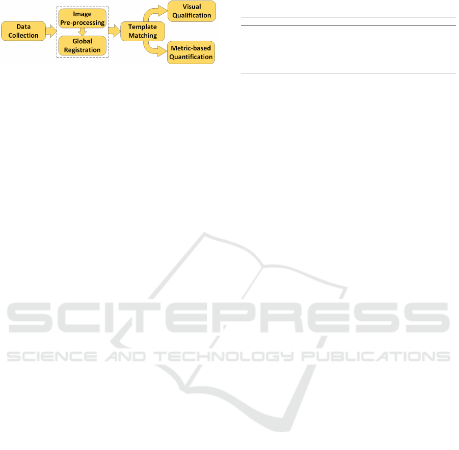
Figure 1: The proposed template matching framework.
larity metrics include the sum of square differences,
the normalised cross-correlation, and the mutual in-
formation for multi-modal image matching, which
can be replaced with superior deep learning mod-
els such as the stacked autoencoders (Wu et al.,
2013; Wu et al., 2015) or convolutional neural net-
works (Gao and Spratling, 2022; Simonovsky et al.,
2016), which have shown promising benefits in multi-
modality matching. By contrast, a feature-based
pipeline starts with extracting discriminative features,
including point, line, and surface, and then match-
ing features using a similarity metric between fea-
tures (Yang et al., 2017). In this category, learning-
based methods, such as deep learning, could be sub-
stituted with traditional frameworks for feature ex-
traction (Barroso-Laguna et al., 2019), feature repre-
sentation (Luo et al., 2019), and similarity measure-
ment (Wang et al., 2017). Methods in this category
can be classified into supervised (Zhang et al., 2017),
self-supervised (Zhang and Rusinkiewicz, 2018), and
unsupervised (Ono et al., 2018) groups based on
whether the feature detectors are trained with or with-
out human annotations.
Co-registration of FLIM and histology images
must be applied to fully understand and reveal the
non-fluorescent features of the investigated tissue
(Wang et al., 2022a). A fundamental step before em-
ploying the registration method is template matching
with the aim of locating a patch in a whole-slide his-
tology image corresponding to the autofluorescence
image. We introduce a new framework for template
matching two image modalities, autofluorescence in-
tensity and bright-field histology. Autofluorescence
intensity images are more appropriate for template
matching than lifetime images because both autoflu-
orescence intensity and histology images have sim-
ilar morphological forms, compared to lifetime im-
ages with visually much fewer structures. As the aut-
ofluorescence intensity image represents a summation
of lifetime data, registering intensity images implic-
itly allows for registering its corresponding lifetime.
The proposed framework comprises different steps,
including image preparation, image pre-processing
to improve image quality, global registration to cor-
rect misalignments, and template matching, which lo-
cates the small histology patch in the whole-slide im-
Table 1: The Wide-field dataset information.
Patient ID Autofluorescence size (pixels) Histology size (pixels)
CR64B 14,043 × 15,008 14,729 × 15,354
CR69B 16,017 × 11,289 17,600 × 13,553
CR64A 17,010× 11, 284 18,494 × 11,335
CR72A 14,019× 13, 775 18,641 × 17,408
CR72B 14,037 × 16,229 13,754 × 17,365
CR91A 12,039× 11, 303 17,780 × 17,573
age. Figure 1 depicts the schematic representation
of the proposed framework. In such a framework,
it is crucial to distinguish whether template match-
ing results are correct. This is very challenging since
FLIM and histology images differ regarding the field
of view, structure, and colours. To this end, we pro-
vide extensive experiments on the impact of different
metrics for discriminating well-matched from poorly-
matched results.
The structure of this paper is organised as fol-
lows. The proposed template matching framework,
along with different quantitative metrics, is presented
in Section 2. Experimental results related to quantify-
ing template matching for discriminating correct re-
sults are provided and discussed in Section 3. Finally,
Section 4 draws the conclusion and future work.
2 PROPOSED METHOD
The proposed template matching framework consists
of four fundamental stages. (1) Raw autofluorescence
intensity and histology images of human lung tis-
sues were collected. (2) Pre-processing is required
for autofluorescence intensity and histology images to
improve their quality and prepare them for template
matching. (3) Global registration must be applied to
correct misalignments between autofluorescence in-
tensity and histology images. (4) Finally, template
matching is used to locate the best patch from the
whole-histology image corresponding to the autoflu-
orescence intensity tile. We introduce various metrics
to quantify the correctness of template matching re-
sults related to the autofluorescence images.
2.1 Data Collection
This research collected human lung tissue samples
from six patients, including normal and cancerous
ones from the Queen’s Medical Research Institute
at the University of Edinburgh. All tissues were
processed through the standard procedure and used
the same hardware configurations to ensure quality-
consistent images. A collection of autofluorescence
intensity images, named the Wide-field dataset, was
captured by an Akoya Vectra Polaris multi-spectral
slide scanner using a standard DAPI filter. The spatial
Quantification of Matching Results for Autofluorescence Intensity Images and Histology Images
707

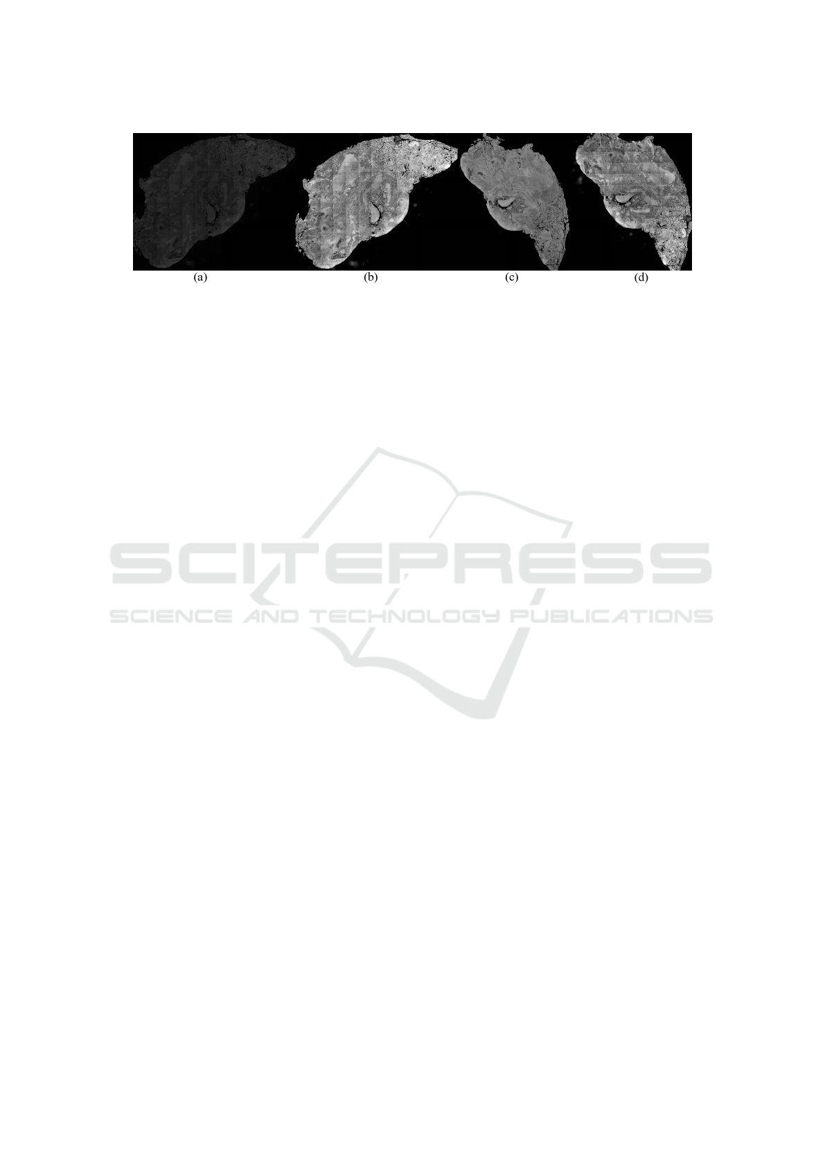
Figure 2: The pre-processing and global registration result: (a) the autofluorescence intensity image, (b) the pre-processed
autofluorescence intensity image, (c) the histology image as the fixed image for registration, (d) the registered intensity image.
resolution for the autofluorescence intensity images
is 0.4541 nm. Table 1 provides further details about
our dataset. The character A or B at the end of the
patient ID indicates whether the tissue is normal or
cancerous. As can be seen, the autofluorescence in-
tensity images of this dataset cover the entire tissue
section with different sizes. Therefore, it is necessary
to extract small-size intensity tiles from the whole-
intensity image and prepare them for template match-
ing. Regarding the second modality, H&E stained im-
ages also went through the standard procedures for
staining and digitalisation to avoid any artefacts/noise
introduced through the procedures. They were col-
lected through a bright-field microscope, Zeiss Axio
Scan.Z1, with a spatial resolution of 0.5009 nm. The
data is confidential from ongoing projects but may be
publicly available in the future.
2.2 Image Pre-Processing
Histology Images. With the help of QuPath and Im-
ageJ software, all histology images were prepared so
that histology images corresponding to autofluores-
cence intensity images were cropped and saved us-
ing TIF format for further processing. The histology
images are then converted to greyscale, followed by
their intensity values being reversed to have a black
background similar to the autofluorescence intensity.
Autofluorescence Intensity Images. Pre-processing
of autofluorescence intensity images is essential to
eliminate the effect of the data distribution variations
due to the nature of the tissues (Wang et al., 2022b).
The image intensity of the autofluorescence image is
first converted from 16 bits to 8 bits, and then con-
trast enhancement using histogram-stretching (Sonka
et al., 2014) is applied to minimise the impact caused
by autofluorescence. Finally, 0.05% of the lowest and
highest intensity values are saturated and clipped to
fall within the normal intensity range (0,255). Fig-
ure 2 (a) and (b) show the raw and the pre-processed
autofluorescence images. Intensity tiles extraction is
another step that must be applied to the intensity im-
age to obtain small-size tiles that enable their use for
template matching. To this end, the intensity tiles are
extracted from the wide-field intensity image in three
sizes: 512 × 512, 1024 × 1024, and 2048 ×2048 pix-
els with 5% overlapping. During this process, inten-
sity tiles that contained more than 50% of background
pixels were removed.
2.3 Global Registration
Since template matching employs pixel-level correla-
tion as a similarity measurement, it is crucial to reg-
ister the histology and autofluorescence intensity im-
ages globally. Pre-processing steps, including inten-
sity inversion for histology images and data normali-
sation for wide-field intensity images, were first em-
ployed to prepare images for registration. Then, the
intensity image is registered to the coordinate space
of the corresponding histology image using Similar-
ity transformation in Matlab R2022b to correct trans-
lation, rotation, and re-scaling. The histology image,
Figure 2 (c), is set as the reference (fixed) image, and
the pre-processed autofluorescence intensity image,
Figure 2 (b), is registered to the coordinate space of
the histology image, where the result of registration is
depicted in Figure 2 (d). Note that since the histology
image covers the entire tissue, the global registration
occurred on the whole-intensity image before extract-
ing the small-size intensity tiles. For the sake of clar-
ity, Figure 3 draws all steps related to pre-processing
and global registration. Finally, the pre-processed his-
tology image and autofluorescence intensity tiles are
input into the next stage, template matching.
2.4 Template Matching
A fundamental step in the co-registration of autofluo-
rescence and histology images is multi-modality im-
age matching, which refers to identifying and link-
ing similar structures from two images with differ-
ent appearances. Matching a histology image with
autofluorescence intensity tiles requires cropping the
ICPRAM 2024 - 13th International Conference on Pattern Recognition Applications and Methods
708

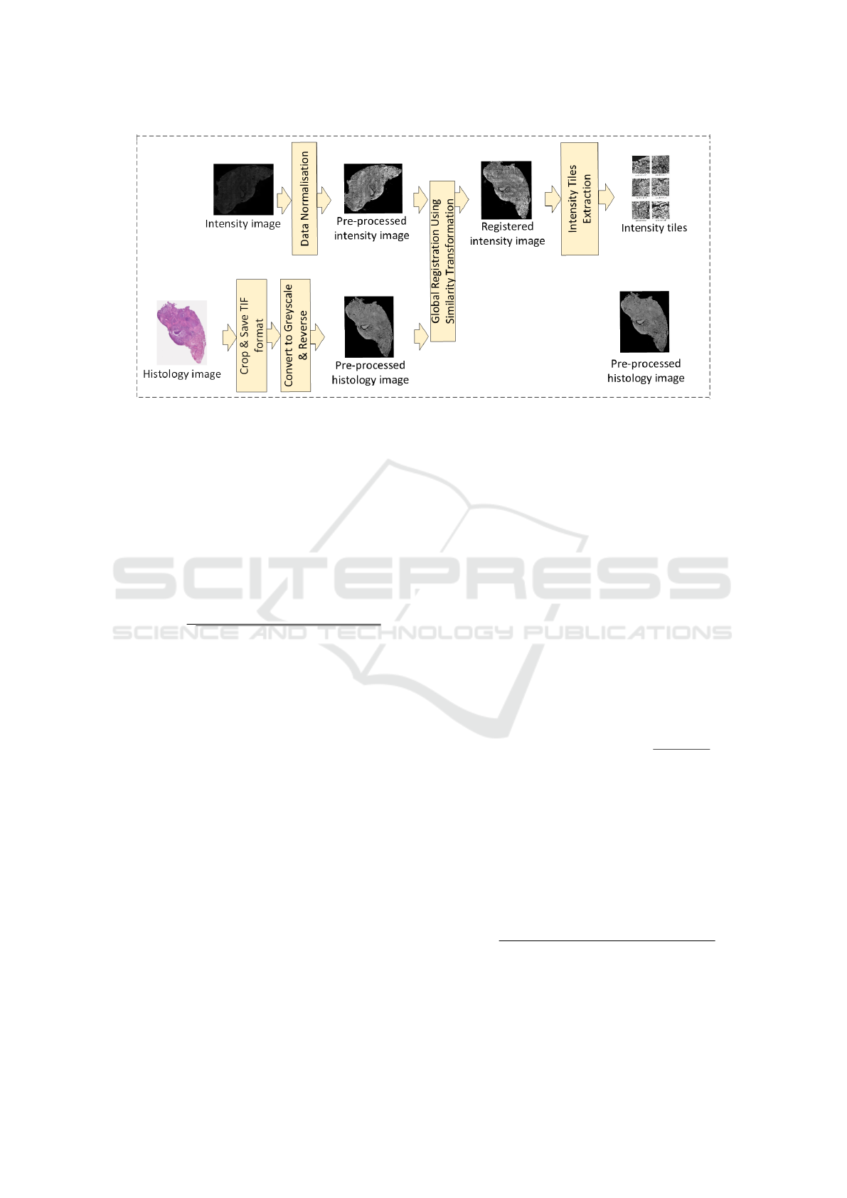
Figure 3: Schematic diagram of all steps related to pre-processing and global registration.
histology patch corresponding to a specific intensity
tile. The appropriate selection of similarity metrics is
crucial to the success of template matching. This pa-
per uses template matching based on Zero-mean Nor-
malised Cross-Correlation (ZNCC) (Stefano et al.,
2005) to locate the corresponding histology patch
from the whole-slide image. The ZNCC value at the
point (x,y) between the searching image (H), whole-
histology image, and the autofluorescence intensity
tile as template image (I
T
) is calculated as:
ZNCC(x,y) =
∑
x
′
,y
′
((I
T
(x
′
,y
′
)−
¯
I
T
)·(H(x+x
′
,y+y
′
)−
¯
H))
q
∑
x
′
,y
′
(I
T
(x
′
,y
′
)−
¯
I
T
)
2
·
∑
x
′
,y
′
(H(x+x
′
,y+y
′
)−
¯
H)
2
(1)
where x
′
= 0,..., w − 1 and y
′
= 0,..., h − 1, while w
and h correspond to the length and width of the tem-
plate image, respectively, and are equal to 512. Also,
¯
I
T
and
¯
H stand for the mean grey values of the corre-
sponding images, respectively. Therefore, the corre-
lation matrix between each autofluorescence intensity
tile with size 512 × 512 pixels and the correspond-
ing patch extracted from the whole-histology image
is calculated using ZNCC. The maximum entry of
this matrix represents the histology patch with the
highest possibility of matching the autofluorescence
intensity tile. Since the row and column indices of
the maximum entry have been saved, we can crop the
histology-matched patch with a size of 512×512 pix-
els from the row and column numbers of the whole-
histology image and obtain the template matching re-
sult.
2.5 Quantification of the Results
After obtaining the template matching results, we
need quantitative metrics to assess the matching qual-
ity of the extracted histology patches. This sec-
tion provides different metrics based on structural
information, entropy, and context-specific contents
to quantify the accuracy of template matching re-
sults. The most common similarity metrics employed
for multi-modal registration are Normalised Cross-
Correlation (NCC), Mutual Information (MI), and
Normalised Mutual Information (NMI) (Mench
´
on-
Lara et al., 2023). Similarly, we use these metrics
to quantify our matching results. However, accord-
ing to our matching outcomes, the ZNCC variation of
cross-correlation, defined in Eq. 1, is better suited for
template matching than NCC. The MI and NMI use
the statistical relationship between images to achieve
multi-modality image registration (Maes et al., 1997).
For the histology-matched patch image I
h
extracted
by the template matching method and the intensity
tile I
T
, the MI can be calculated by the normalised
histogram of the images as follows:
MI =
∑
a∈A
I
h
∑
b∈A
I
T
P
I
h
I
T
(a,b)· log
2
(
P
I
h
I
T
(a,b)
P
I
h
(a)·P
I
T
(b)
) (2)
where P
I
h
and P
I
T
are the marginal histograms of the
two images, and P
I
h
I
T
is the joint histogram. P
I
h
I
T
is a
2-dimensional matrix that holds the normalised num-
ber of intensity values (a,b) observed in I
h
and I
T
. In
addition, A
I
h
and A
I
T
are discrete bins of intensity val-
ues of the histology-matched patch and the template
image, respectively. The normalised mutual informa-
tion is defined as follows, where all terms were intro-
duced in Eq. 2:
NMI =
∑
a∈A
I
h
∑
b∈A
I
T
P
I
h
I
T
(a,b)·log
2
(P
I
h
(a)·P
I
T
(b))
∑
a∈A
I
h
∑
b∈A
I
T
P
I
h
I
T
(a,b)·log
2
(P
I
h
I
T
(a,b)
(3)
Kullback Leibler Divergence. One main limitation
of the metrics described above for registration pur-
poses in clinical applications is the context-free nature
of the measures. Context-free means that they do not
Quantification of Matching Results for Autofluorescence Intensity Images and Histology Images
709

consider the registration’s underlying context, such as
the intensity mapping relationship of the images and
the statistics of the modalities to be registered. To
move towards context-specific metrics and produce
accurate and reliable registration results, it is required
to use prior knowledge of image content (Crum et al.,
2003). The Kullback Leibler Divergence (KLD) met-
ric, which uses the prior knowledge of the expected
joint intensity histogram to guide the multi-modal
registration, was proposed (Guetter et al., 2005; Chan
et al., 2003). Consequently, we employed this valu-
able metric to quantify the template matching results
and distinguish the correctness of matching results.
To this end, the probability distribution for the inten-
sities of the histology-matched patch and autofluores-
cence intensity tile is calculated by their normalised
histograms. The evaluation metric based on KLD be-
tween the histology-matched patch image I
h
and the
autofluorescence intensity tile I
T
is defined as follows
while using I
h
as the reference image:
KLD(I
T
∥I
h
) = −
∑
i
P
I
T
i
(x) ·log P
I
h
i
(x) +
∑
i
P
I
T
i
(x) ·log P
I
T
i
(x) (4)
where P
I
T
i
and P
I
h
i
represent the probability distribu-
tion of intensities for the autofluorescence intensity
tile and the histology-matched patch, respectively. As
a result, the maximum probability distribution dis-
similarity between the histogram of the histology-
matched patch P
I
h
and the autofluorescence intensity
tile P
I
T
is calculated using Eq. 4. Due to the non-
symmetric nature of the KLD, the symmetrical ver-
sion is calculated using Eq. 5, in which the reference
image is once set as the histology-matched patch and,
once again, set as the autofluorescence intensity tile.
The mean of these two measures is reported as the
symmetric version of KLD (S
KLD
).
S
KLD
= 0.5 ×(KLD(I
T
∥I
h
) + KLD(I
h
∥I
T
)) (5)
Misfit-Percent. Misfit-percent is an additional help-
ful metric to determine the correctness of template
Table 2: The number and rate of successful matching results
based on visual inspection using different tile sizes.
Patient ID 512 × 512 1024 × 1024 2048 × 2048
CR64B 186/220 120/143 33/34
84% 84% 97%
CR69B 65/276 25/65 10/14
24% 38% 71%
CR64A 149/235 93/118 30/31
63% 78% 96%
CR72A 60/196 16/50 5/13
30% 32% 38%
CR72B 95/260 70/135 26/38
36% 51% 68%
CR91A 133/233 82/93 22/22
57% 88% 100%
matching outcomes. Compared to KLD, misfit-
percent is completely normalised in nature, allowing
its use for distinguishing the correctness of matching
results simply by thresholding (Taimori et al., 2023).
This metric calculates the sum of the absolute error
between the probability distribution of the histology-
matched image and the autofluorescence intensity tile
image. Then, it divides the outcome by the union of
the distributions to normalise it. We consider the nor-
malised histogram as the probability distribution for
the intensities of images. The misfit-percent between
the histology-matched patch I
h
and the autofluores-
cence intensity tile I
T
is defined by:
Mis f it − percent =
Σ
N−1
i=0


P
I
h
i
− P
I
T
i


Σ
N−1
i=0
max(P
I
h
i
· P
I
T
i
)
(6)
where N is the total number of intensity values.
3 EXPERIMENTAL RESULTS
3.1 Visual Qualification
To assess template-matching results, we visually
compared and classified the matching outcomes as
correct or incorrect. Although the number of patients
is limited, a sufficient number of autofluorescence in-
tensity tiles, a total of 2,170, were extracted from
the whole-intensity images. The number and percent-
age of accurate matching results based on a visual in-
spection with different tile sizes for each patient are
reported in Table 2. Since some intensity tiles are
homogeneous and lack any visible underlying struc-
tures, template matching fails. We empirically re-
solved this issue by applying template matching to
tiles extracted with a larger size, such as 1024 × 1024
or 2048 × 2048 pixels. As the size of the tile in-
creased, it became more likely that apparent struc-
tures would appear in the autofluorescence intensity
tiles. As seen in Table 2, the number of success-
ful matched results rises significantly as the tile size
increases. As noted, we classified the matching re-
sults based on a visual inspection, which was time-
consuming and laborious. Therefore, evaluating tem-
plate matching results quantitatively and distinguish-
ing correct from incorrect ones is imperative.
3.2 Metric-Based Quantification
NCC, MI and NMI Metrics. An evaluation of tem-
plate matching results based on three metrics, ZNCC,
NMI, and MI, is depicted in Figure 4 (a). This fig-
ure depicts the range of the three metrics for tem-
plate matching results: well-matched (blue box) and
ICPRAM 2024 - 13th International Conference on Pattern Recognition Applications and Methods
710

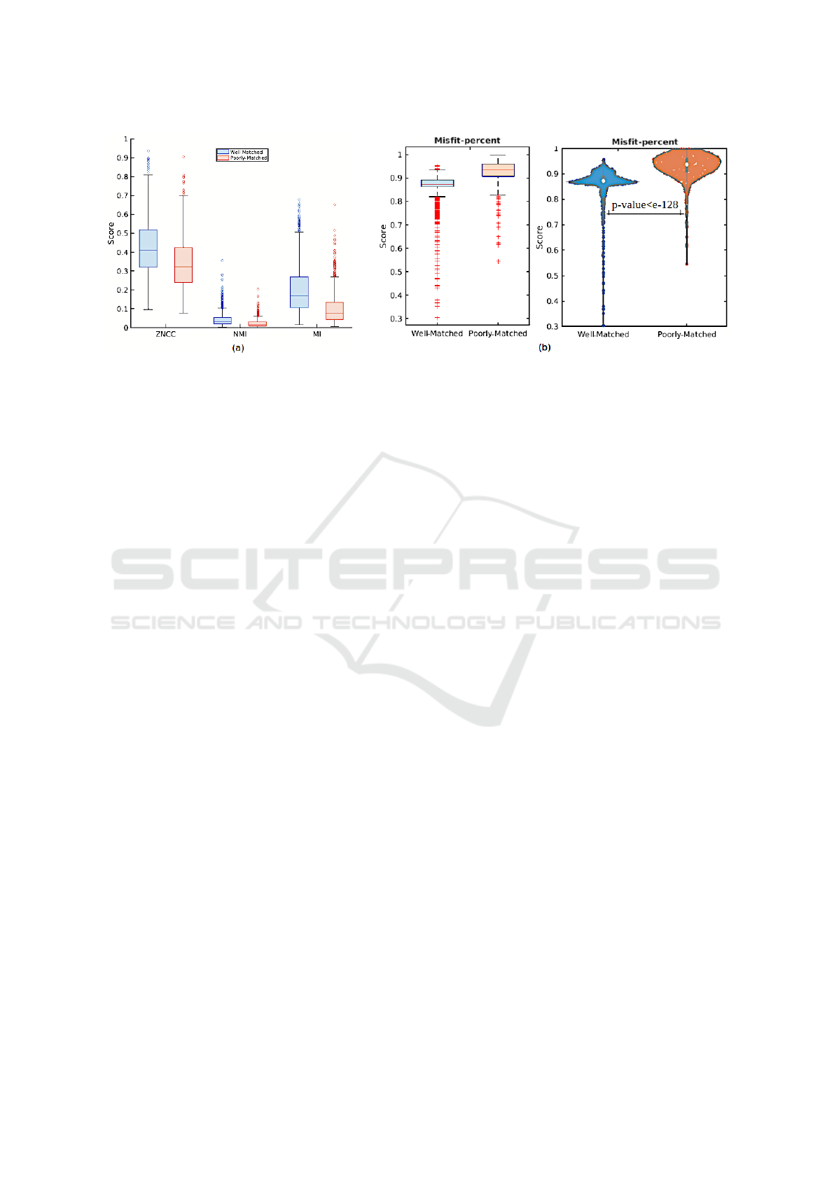
Figure 4: Statistical comparison of well- and poorly-matched results based on (a) ZNCC, NMI, and MI metrics. (b) Statistical
(left) and density (right) comparison based on the misfit-percent.
poorly-matched (red box). It is evident that we cannot
distinguish between correct matching results from in-
correct ones using these three metrics, given that the
range of scores for well-matched and poorly-matched
for each metric has considerable overlap. Therefore,
these metrics failed for our microscopic images, even
though they are most common for multi-modality
template matching.
Kullback Leibler Divergence Metric. Figure 5
(a) illustrates the statistical comparison of well-
and poorly-matched results based on symmetric and
asymmetric KLD measures. To calculate asymmet-
ric KLD, we set the histology-matched patches as
reference images. As can be seen, the capability
of KLD (symmetric and asymmetric) for distinguish-
ing the correct matched results is superior, as there
is no meaningful overlap between well- and poorly-
matched. Figure 5 (a) shows that we can determine a
well-matched outcome if its KLD score is lower than
a threshold, while a higher KLD score indicates an
incorrect match. This threshold can be determined
around 1 and 2 for symmetric and asymmetric KLD,
respectively. In addition, based on the KLD scores
shown in Figure 5 (a), there are a few poorly-matched
tiles depicted as outliers, shown as red pluses at the
top of the box median, while their KLD scores are
higher than the box median, so they are classified as
poorly-matched, which is in line with the threshold.
This event also occurred for outliers at the bottom of
the box median, associated with well-matched in the
asymmetric version. Although a limited proportion of
well-matched tiles have high KLD scores in both fig-
ures, we need to find a strategy to reduce these false
negatives as well as a few false positives associated
with poorly-matched results in asymmetric KLD.
To visually demonstrate the distribution of match-
ing results, Figure 5 (b) shows the density compari-
son of well- and poorly-matched outcomes using vi-
olin plots based on symmetric and asymmetric KLD
scores, respectively. As can be seen, there are sig-
nificant differences in the distribution between well-
and poorly-matched groups, especially with regard to
the concentration of data based on median markers.
Furthermore, we utilised a t-test statistical analysis at
0.05 level of significance to determine the extent of
differences observed in Figure 5 (b). The p-values
resulting from the t-test analysis of the null hypoth-
esis are 1.39e − 99 and 1.64e − 180 for symmetric
and asymmetric KLD, respectively. The smaller the
p-value, the stronger the evidence. Therefore, the t-
test analysis states that there is a meaningful differ-
ence in the mean scores of well- and poorly-matched
KLD scores, including both symmetric and asymmet-
ric ones, which is statistically significant and prov-
able. As a result of p-values, the asymmetric KLD
seems to behave slightly better than the symmetric
score. The results also show a more significant gap
between the mean scores for asymmetric KLD than
symmetric KLD and that there are far fewer outliers
in asymmetric KLD associated with false negatives.
Misfit-Percent Metric. Another metric beneficial
for microscopy images is the misfit-percent shown
in Figure 4 (b). As depicted in Figure 4 (b) on the
left, most of the 75% well-matched tiles have misfit-
percent scores lower than 0.9, around the box median,
while this score is higher than 0.9 for most poorly-
matched tiles. Since the distribution of misfit-percent
for well- and poorly-matched results is considerably
different, this metric is highly effective in distinguish-
ing the correct matched results. Meanwhile, there
are some outliers related to the correct results, with
scores lower than 0.9, which corroborates the superi-
ority of this metric, and we can distinguish them with
the simple threshold. However, the outliers related
to the incorrect results with scores lower than 0.9 are
not interesting and are regarded as false positives. We
Quantification of Matching Results for Autofluorescence Intensity Images and Histology Images
711

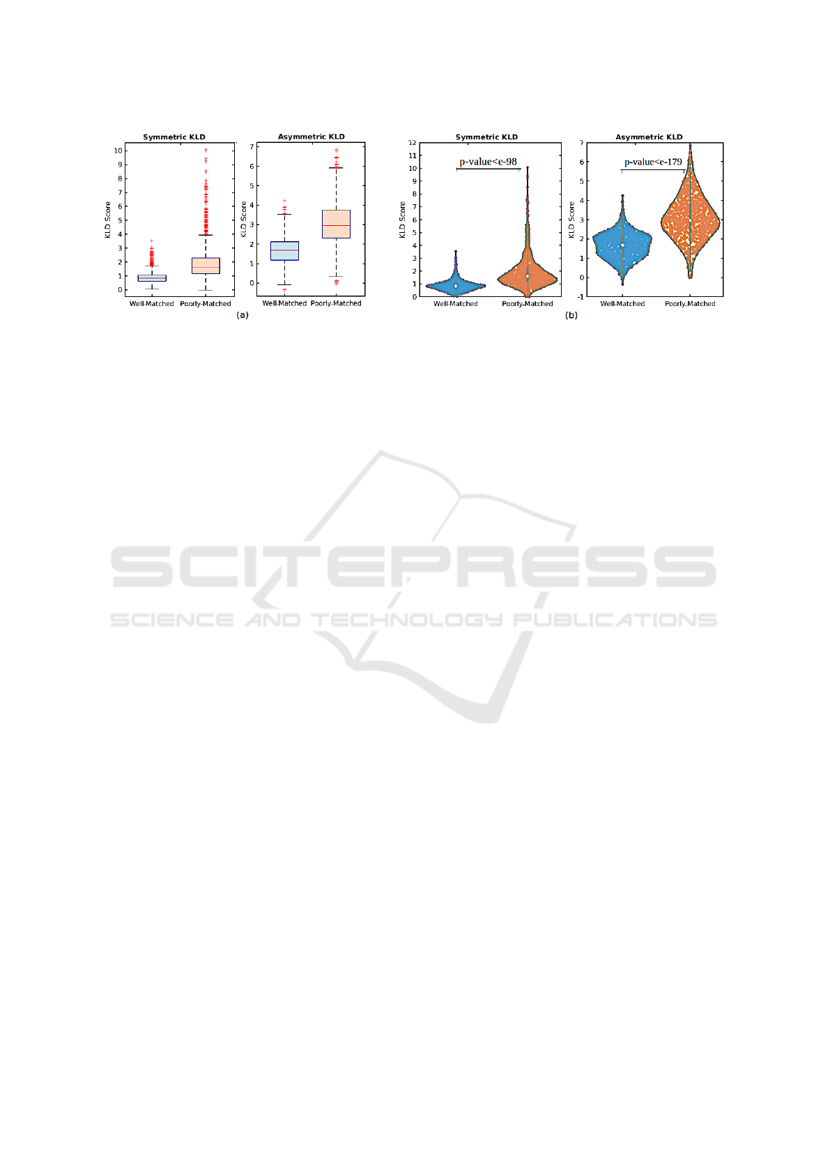
Figure 5: (a) Statistical and (b) density comparison of results based on symmetric and asymmetric KLD.
can use the symmetric KLD scores of corresponding
tiles that aid in discriminating poorly-matched tiles
well. To better visualise, the distribution of tiles based
on their misfit-percent scores is shown in Figure 4
(b) on the right. As can be seen, the distribution of
data between well- and poorly-matched is completely
different. Furthermore, the p-value obtained from
the t-test analysis is 4.36e − 129, which is consider-
ably slight, indicating that the difference between the
misfit-percent scores of well- and poorly-matched is
statistically considerable.
Our extensive experiments demonstrate that com-
bination of the KLD and misfit-percent scores is most
appropriate for differentiating between correct and
incorrect matching results. If the KLD and misfit-
percent scores are lower than the specified thresholds,
the results can be classified as well-matched, and vice
versa as poorly-matched. Regarding false positives
obtained via the misfit-percent metric, we can utilise
the KLD scores of corresponding tiles to address this
issue because the KLD metric behaves well for this
category. Similarly, we can use the misfit-percent of
the corresponding tiles to reduce false negatives, the
issue related to the symmetric and asymmetric KLD
metrics. In this research, we presented a proof of con-
cept, and we do not claim that our thresholds for KLD
and misfit-percent metrics were optimal. To find an
automatic thresholding approach, careful validation
through experiments is necessary.
4 CONCLUSION AND FUTURE
WORK
Although various template matching methods have
recently been introduced, the need to thoroughly
compare metrics to determine whether the template
matching results are accurate is significantly appar-
ent. In this paper, we analysed the results relating to
the impact of different metrics to quantify the correct-
ness of template matching related to autofluorescence
images. Our next step would be to develop a similar-
ity measurement for microscopy images based on the
appropriate metrics described in this research. One
limitation of the current study is the need for a bench-
mark to assess these metrics, although extending our
dataset with more images would be of interest. More-
over, in our future research, we plan to expand the
comparison and quantification to different modalities
of microscopy images.
REFERENCES
Barroso-Laguna, A., Riba, E., Ponsa, D., and Mikolajczyk,
K. (2019). Key. net: Keypoint detection by hand-
crafted and learned cnn filters. In Proceedings of the
IEEE/CVF international conference on computer vi-
sion, pages 5836–5844.
Chan, H.-M., Chung, A. C., Yu, S. C., Norbash, A., and
Wells, W. M. (2003). Multi-modal image registra-
tion by minimizing kullback-leibler distance between
expected and observed joint class histograms. In
2003 IEEE Computer Society Conference on Com-
puter Vision and Pattern Recognition, 2003. Proceed-
ings, pages II–570.
Cheng, X., Zhang, L., and Zheng, Y. (2018). Deep simi-
larity learning for multimodal medical images. Com-
puter Methods in Biomechanics and Biomedical Engi-
neering: Imaging & Visualization, 6(3):248–252.
Crum, W. R., Griffin, L. D., Hill, D. L., and Hawkes, D. J.
(2003). Zen and the art of medical image registration:
correspondence, homology, and quality. NeuroImage,
20(3):1425–1437.
Daga, A. P. and Garibaldi, L. (2020). Ga-adaptive tem-
plate matching for offline shape motion tracking based
on edge detection: Ias estimation from the survishno
2019 challenge video for machine diagnostics pur-
poses. Algorithms, 13(2):33.
Datta, R., Heaster, T. M., Sharick, J. T., Gillette, A. A.,
and Skala, M. C. (2020). Fluorescence lifetime imag-
ing microscopy: fundamentals and advances in in-
strumentation, analysis, and applications. Journal of
biomedical optics, 25(7):071203–071203.
ICPRAM 2024 - 13th International Conference on Pattern Recognition Applications and Methods
712

Gao, B. and Spratling, M. W. (2022). Robust template
matching via hierarchical convolutional features from
a shape biased cnn. In The International Confer-
ence on Image, Vision and Intelligent Systems (ICIVIS
2021), pages 333–344.
Guetter, C., Xu, C., Sauer, F., and Hornegger, J. (2005).
Learning based non-rigid multi-modal image registra-
tion using kullback-leibler divergence. In Medical Im-
age Computing and Computer-Assisted Intervention–
MICCAI 2005: 8th International Conference, Palm
Springs, CA, USA, October 26-29, 2005, Proceedings,
Part II 8, pages 255–262.
Haskins, G., Kruecker, J., Kruger, U., Xu, S., Pinto, P. A.,
Wood, B. J., and Yan, P. (2019). Learning deep simi-
larity metric for 3d mr–trus image registration. Inter-
national journal of computer assisted radiology and
surgery, 14:417–425.
Jiang, X., Ma, J., Xiao, G., Shao, Z., and Guo, X. (2021). A
review of multimodal image matching: Methods and
applications. Information Fusion, 73:22–71.
Lin, W., Li, X., Yang, Z., Manga, M., Fu, X., Xiong, S.,
Gong, A., Chen, G., Li, H., Pei, L., Li, S., Zhao,
X., and Wang, X. (2019). Multiscale digital porous
rock reconstruction using template matching. Water
Resources Research, 55(8):6911–6922.
Loeckx, D., Slagmolen, P., Maes, F., Vandermeulen, D., and
Suetens, P. (2009). Nonrigid image registration using
conditional mutual information. IEEE transactions on
medical imaging, 29(1):19–29.
Luo, Z., Shen, T., Zhou, L., Zhang, J., Yao, Y., Li, S., Fang,
T., and Quan, L. (2019). Contextdesc: Local descrip-
tor augmentation with cross-modality context. In Pro-
ceedings of the IEEE/CVF conference on computer vi-
sion and pattern recognition, pages 2527–2536.
Ma, W., Li, W., and Cao, P. (2019). Ranging method of
binocular stereo vision based on random ferns and ncc
template matching. In IOP Conference Series: Earth
and Environmental Science, page 022149.
Maes, F., Collignon, A., Vandermeulen, D., Marchal, G.,
and Suetens, P. (1997). Multimodality image regis-
tration by maximization of mutual information. IEEE
transactions on Medical Imaging, 16(2):187–198.
Marcu, L. (2012). Fluorescence lifetime techniques in med-
ical applications. Annals of biomedical engineering,
40:304–331.
Mench
´
on-Lara, R.-M., Simmross-Wattenberg, F.,
Rodr
´
ıguez-Cayetano, M., de-la Higuera, P. C.,
Mart
´
ın-Fern
´
andez, M.
´
A., and Alberola-L
´
opez, C.
(2023). Efficient convolution-based pairwise elastic
image registration on three multimodal similarity
metrics. Signal Processing, 202:108771.
Ono, Y., Trulls, E., Fua, P., and Yi, K. M. (2018). Lf-
net: Learning local features from images. Advances
in neural information processing systems, 31.
Simonovsky, M., Guti
´
errez-Becker, B., Mateus, D., Navab,
N., and Komodakis, N. (2016). A deep metric for mul-
timodal registration. In Medical Image Computing
and Computer-Assisted Intervention-MICCAI 2016:
19th International Conference, Athens, Greece, Octo-
ber 17-21, 2016, Proceedings, Part III 19, pages 10–
18.
Sonka, M., Hlavac, V., and Boyle, R. (2014). Image
processing, analysis, and machine vision. Cengage
Learning.
Stefano, L. D., Mattoccia, S., and Tombari, F. (2005). Zncc-
based template matching using bounded partial corre-
lation. Pattern recognition letters, 26(14):2129–2134.
Taimori, A., Mills, B., Gaughan, E., Ali, A., Dhaliwal, K.,
Williams, G., Finlayson, N., and Hopgood, J. (2023).
A novel fit-flexible fluorescence imager: Tri-sensing
of intensity, fall-time, and life profile. TechRxiv.
Wang, J., Zhou, F., Wen, S., Liu, X., and Lin, Y. (2017).
Deep metric learning with angular loss. In Proceed-
ings of the IEEE international conference on com-
puter vision, pages 2593–2601.
Wang, Q., Fernandes, S., Williams, G. O., Finlayson,
N., Akram, A. R., Dhaliwal, K., Hopgood, J. R.,
and Vallejo, M. (2022a). Deep learning-assisted co-
registration of full-spectral autofluorescence lifetime
microscopic images with h&e-stained histology im-
ages. Communications biology, 5(1):1119.
Wang, Q., Hopgood, J. R., Fernandes, S., Finlayson, N.,
Williams, G. O., Akram, A. R., Dhaliwal, K., and
Vallejo, M. (2022b). A layer-level multi-scale archi-
tecture for lung cancer classification with fluorescence
lifetime imaging endomicroscopy. Neural Computing
and Applications, 34(21):18881–18894.
Wu, G., Kim, M., Wang, Q., Gao, Y., Liao, S., and
Shen, D. (2013). Unsupervised deep feature learn-
ing for deformable registration of mr brain images.
In Medical Image Computing and Computer-Assisted
Intervention–MICCAI 2013: 16th International Con-
ference, Nagoya, Japan, September 22-26, 2013, Pro-
ceedings, Part II 16, pages 649–656.
Wu, G., Kim, M., Wang, Q., Munsell, B. C., and Shen, D.
(2015). Scalable high-performance image registration
framework by unsupervised deep feature representa-
tions learning. IEEE transactions on biomedical engi-
neering, 63(7):1505–1516.
Yang, K., Pan, A., Yang, Y., Zhang, S., Ong, S. H., and
Tang, H. (2017). Remote sensing image registra-
tion using multiple image features. Remote Sensing,
9(6):581.
Ye, Y., Bruzzone, L., Shan, J., Bovolo, F., and Zhu, Q.
(2019). Fast and robust matching for multimodal re-
mote sensing image registration. IEEE Transactions
on Geoscience and Remote Sensing, 57(11):9059–
9070.
Zhang, L. and Rusinkiewicz, S. (2018). Learning to detect
features in texture images. In Proceedings of the IEEE
conference on computer vision and pattern recogni-
tion, pages 6325–6333.
Zhang, X., Yu, F. X., Karaman, S., and Chang, S.-F. (2017).
Learning discriminative and transformation covariant
local feature detectors. In Proceedings of the IEEE
conference on computer vision and pattern recogni-
tion, pages 6818–6826.
Quantification of Matching Results for Autofluorescence Intensity Images and Histology Images
713