
Multi-Granular Evaluation of Diverse Counterfactual Explanations
Yining Yuan
1
, Kevin McAreavey
1
, Shujun Li
2
and Weiru Liu
1
1
School of Engineering Mathematics and Technology, University of Bristol, U.K.
2
School of Computing, University of Kent, U.K.
Keywords:
Counterfactual Explanations, Explainable AI.
Abstract:
As a popular approach in Explainable AI (XAI), an increasing number of counterfactual explanation algo-
rithms have been proposed in the context of making machine learning classifiers more trustworthy and trans-
parent. This paper reports our evaluations of algorithms that can output diverse counterfactuals for one in-
stance. We first evaluate the performance of DiCE-Random, DiCE-KDTree, DiCE-Genetic and Alibi-CFRL,
taking XGBoost as the machine learning model for binary classification problems. Then, we compare their
suggested feature changes with feature importance by SHAP. Moreover, our study highlights that synthetic
counterfactuals, drawn from the input domain but not necessarily the training data, outperform native counter-
factuals from the training data regarding data privacy and validity. This research aims to guide practitioners in
choosing the most suitable algorithm for generating diverse counterfactual explanations.
1 INTRODUCTION
With machine learning models being deployed widely
across various sectors in decision-making, the predic-
tions and decisions made by these models are grow-
ing in influence and impact. Explanations for these
models’ outputs are crucial for domains where users
need to build trust in the model and prefer more trans-
parency in decision-making, such as healthcare, credit
loans, etc. Explaining decisions made by AI and ma-
chine learning models can also help ensure compli-
ance with laws such as the GDPR regulating auto-
mated decision-making (Wachter et al., 2017).
Background: Explainability can be realized
through inherently interpretable models like linear
and logistic regression, etc., or via post-hoc ex-
planations, which also work for black-box machine
learning models like random forests and neural net-
works. Post-hoc explanation approaches can be
model-specific, including visual explanations and
model simplification, or model-agnostic, including
feature importance and local explanations (Verma
et al., 2020). Feature importance can be calculated by
SHAP (Lundberg and Lee, 2017). Local explanations
can be further divided into two main types: approx-
imation methods that aim to mimic the behaviour of
the model locally, such as LIME (Ribeiro et al., 2016),
and example-based methods that return nearby data
points with differing predictions, such as Counterfac-
tual Explanations (CFEs) (Poyiadzi et al., 2020).
Counterfactual explanations are a popular ap-
proach in XAI. These are sometimes said to offer ac-
tionable insights by suggesting modifications to a data
point or, alternatively, an instance to alter its classi-
fication outcome. For instance, consider a loan ap-
plication case where an individual is denied a loan
based on a machine learning model’s prediction. That
individual would naturally want to understand the
changes they could make to secure approval. A CFE
could inform this applicant that increasing their in-
come by a certain amount or acquiring two additional
years of education would have led to loan approval
(Verma et al., 2020).
Understanding the importance of features in a
model’s prediction is a crucial aspect of XAI. Tools
like SHAP provide consistent measures of feature im-
portance, which affect the outcome of a prediction.
While SHAP values highlight the importance, the out-
come of changing these feature values is crucial for
CFEs. Even if a feature is deemed important, chang-
ing it may not lead to a different prediction. DiCE
methods consider feature weight either by using dis-
tances or manual entries (Mothilal et al., 2020). The
interplay between feature importance and actionabil-
ity can be pivotal in ensuring that the recommenda-
tions provided by CFEs are both influential and feasi-
ble for end-users.
Challenges of CFEs: In real-world applications,
186
Yuan, Y., McAreavey, K., Li, S. and Liu, W.
Multi-Granular Evaluation of Diverse Counterfactual Explanations.
DOI: 10.5220/0012349900003636
Paper published under CC license (CC BY-NC-ND 4.0)
In Proceedings of the 16th International Conference on Agents and Artificial Intelligence (ICAART 2024) - Volume 2, pages 186-197
ISBN: 978-989-758-680-4; ISSN: 2184-433X
Proceedings Copyright © 2024 by SCITEPRESS – Science and Technology Publications, Lda.
CFEs often need to adhere to specific constraints, en-
suring that the recommended changes are not only ac-
tionable but also realistic and aligned with common-
sense understanding. Using counterfactuals taken
from the training data can significantly reduce the run
time and enhance the plausibility of the explanations,
where plausibility refers to how realistic the coun-
terfactual explanation is concerning the data mani-
fold (Goethals et al., 2023). CFEs that return data
points that existed in the original dataset as explana-
tions are known as native counterfactuals (Goethals
et al., 2023). CFEs not relying on specific examples
from the training set are known as synthetic counter-
factuals (Keane and Smyth, 2020). However, there’s a
privacy risk associated with counterfactual algorithms
that use native instance-based strategies. They can
potentially reveal private information about other de-
cision subjects, such as someone’s grades in educa-
tional decisions or income in credit scoring decisions
(Vo et al., 2023). While native counterfactuals can re-
veal records from the training dataset, synthetic coun-
terfactuals do not have this risk. However, techniques
that generate synthetic counterfactuals are also vul-
nerable to privacy attacks, such as model extraction
(Goethals et al., 2023).
The motivation behind this research is to study
the advantages and limitations of CFE algorithms cur-
rently available. There is a growing consensus on
the advantages of producing multiple CFE alterna-
tives rather than a single CFE, where a higher diver-
sity value is desirable (Molnar, 2022). Such diversity
provides decision-makers with distinct alternatives to
reach the desired outcome.
In this research, we selected DiCE and Alibi, the
popular Python libraries on GitHub capable of gener-
ating diverse counterfactuals for a single instance for
comparison. Notably, DiCE-Random, DiCE-Genetic
and DiCE-KDTree are under the Diverse Counterfac-
tual Explanations (DiCE) framework, which offers
a unique opportunity to explore the different algo-
rithms (random sampling, genetic algorithm, and k-
dimension trees) within a unified framework. Alibi-
CFRL is a reinforcement learning-based method in-
tegrated into Alibi. Here, DiCE-KDTree only out-
puts native instances in the training set, while other
algorithms return synthetic data points. The overall
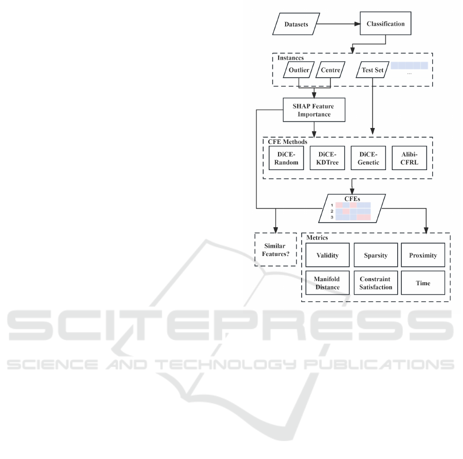
workflow of our evaluation is shown in Figure 1. Our
comparison stands to benefit end-users who leverage
these explanations for informed decision-making and
data scientists who can harness the derived insights
to build models that are both more robust and more
explainable.
Based on the above background, this research has
the following contributions:
Figure 1: Overview of the evaluation process.
• We compared SHAP local explanation and other
CFE algorithms on the central data point and the
outlier data point within the dataset. Our central
data point is the one closest to the mean centre of a
dataset, while an outlier is the data point that devi-
ates the most from the mean centre. Our compar-
ison shows a disconnect between SHAP feature
importance and the feature alterations in the CFEs
by the four algorithms we examined. Specifi-
cally, the features identified as most important by
SHAP do not consistently match those altered in
the CFEs.
• We evaluated the actionability of four CFE al-
gorithms on the unfavourable class. In our con-
text, the unfavourable class means being rejected
for a loan and having a lower income in census
data. We discovered that Alibi-CFRL and DiCE-
Random outperform other algorithms in different
metrics.
• We emphasized the importance of synthetic coun-
terfactuals instead of native counterfactuals in
CFEs for data privacy.
Multi-Granular Evaluation of Diverse Counterfactual Explanations
187

2 RELATED WORK
2.1 CFEs Methods
Native Counterfactual Methods: CFEs that re-
turn data points that existed in the original dataset
as explanations are known as native counterfactu-
als (Goethals et al., 2023). Poyiadzi et al. (2020)
proposed FACE, which employs Dijkstra’s algorithm
to identify the most direct route connecting close
data points based on density-weighted distances and
identifies counterfactuals using model predictions and
density thresholds (Poyiadzi et al., 2020). As a re-
sult, this technique does not create new data points.
KDTree prototype (Van Looveren and Klaise, 2021)
uses a k-dimension tree to partition training data
based on feature values, identifying nearest neigh-
bours to the input instance and sourcing counterfac-
tuals directly from these neighbours, ensuring that
they reflect the original feature distributions and meet
specified constraints.
Genetic-based Methods: Genetic-based CFE
methods generate synthetic CFEs. The genetic algo-
rithms use mutation and crossover to evolve potential
solutions, optimizing the predicted probability based
on certain constraints and cost functions to provide
synthetic CFEs. GIC (Lash et al., 2017) introduces
real-valued heuristic-based methods, including hill-
climbing, local search, and genetic algorithms. CER-
TIFAI (Sharma et al., 2019) is a meta-heuristic evolu-
tionary algorithm that begins by producing a random
set of data points that do not share the same predic-
tion as the input data point. MOC (Dandl et al., 2020)
employs mixed integer evolutionary strategies to han-
dle both discrete and continuous search spaces for
generating CFEs. Compared with previous methods,
GeCO achieves real-time performance and a complete
search space by incorporating two novel optimiza-
tions. ∆-representation groups candidates by differ-
ing features, using compact tables for memory and
performance gains. Classifier Specialization via Par-
tial Evaluation streamlines classifiers to only assess
varying features (Schleich et al., 2021).
Prototype-based Methods: Both prototype-
based methods and reinforcement learning-based
methods below generate CFEs. Based on the origi-
nal loss term by (Wachter et al., 2017), Van Looveren
and Klaise (2021) used a prototype loss term to guide
the perturbations towards an interpretable counterfac-
tual. The prototype for each class can be defined us-
ing an encoder, where the prototype is the average en-
coding of instances belonging to that class. Duong et
al. (2021) proposed a prototype-based method to en-
sure that the counterfactual instance respects the con-
straints and is interpretable.
Reinforcement Learning-based Methods:
Samoilescu et al. (2021) introduced a deep re-
inforcement learning approach. The significant
advantages of this method are its fast counterfactual
generation process and its flexibility in adapting to
other data modalities like images. Verma et al. (2022)
proposed FASTAR, another approach that translates
the sequential algorithmic recourses problem into
a Markov Decision Process that uses reinforcement
learning to generate amortized CFEs.
To summarize, the methods outlined above mostly
generate synthetic CFEs than finding native CFEs.
Our analysis indicates a prevailing trend among re-
cent CFE algorithms, which lean more toward syn-
thetic than native. However, the reasons driving this
shift are seldom explored in the existing literature.
2.2 Quantitative Properties
In this subsection, we look into several quantitative
properties, including validity, sparsity, proximity, data
manifold, actionability and diversity.
Validity: CFE methods are unsound in that they
may return data points that do not have the desired
target label. A counterfactual correctly classified into
the desired class while satisfying hard constraints is
considered a valid counterfactual. Popular hard con-
straints specify immutable features, feature ranges
(Mothilal et al., 2020) and the direction of feature
value change (Samoilescu et al., 2021). Validity mea-
sures the proportion of instances within the test set for
which sound CFEs can be generated. A higher valid-
ity ratio indicates better performance because a larger
proportion of generated counterfactuals have the op-
posite class label to the original (Samoilescu et al.,
2021).
Sparsity: Sparsity refers to the number of fea-
tures changed to obtain a counterfactual. Addition-
ally, a CFE x
′
is minimally sparse given input x if
it minimizes the Hamming distance d(x, x
′
) = |{i :
i = 1, 2, ..., n : x
i
̸= x
′
i
}|. This is considered be-
cause shorter answers have been argued to be eas-
ier for people to understand (Naumann and Ntoutsi,
2021). Sparsity is typically enforced by methods us-
ing solvers (Karimi et al., 2020) or by constraining the
L
0
norm for black-box methods (Dandl et al., 2020).
L
0
norm counts the number of non-zero elements in a
vector. Gradient-based methods often use the L
1
norm
between counterfactuals and input data points. The
L
1
norm of a vector is the sum of the absolute values
of its components. Some approaches change a fixed
number of features (Keane and Smyth, 2020), adjust
features iteratively (Le et al., 2020), or flip the min-
ICAART 2024 - 16th International Conference on Agents and Artificial Intelligence
188

imal possible split nodes in a decision tree (Guidotti
et al., 2018) to induce sparsity.
Proximity: Proximity refers to the closeness
between a counterfactual and the original instance
(Brughmans et al., 2023). To be useful, counterfac-
tuals should ideally be close to the original data point.
The smaller the distance between the counterfactual
and the original data point, the better. Distance met-
rics such as the Euclidean distance or Mahalanobis
distance are often used for this purpose and are of-
ten measured separately for numerical and categorical
features (Verma et al., 2020).
Data Manifold Closeness: Data manifold means
the closeness to the training data distribution (Verma
et al., 2020; Verma et al., 2022). Several approaches
address data manifold adherence using techniques
such as training VAEs on the data distribution (Ma-
hajan et al., 2019), constraining the counterfactual
distance from the nearest training data points (Dandl
et al., 2020), sampling points from the latent space
of a VAE (Pawelczyk et al., 2020), using an en-
semble model to capture predictive entropy (Schut
et al., 2021), or applying Kernel Density Estimation
(F
¨
orster et al., 2021) and Gaussian Mixture Mod-
els (Artelt and Hammer, 2021b). Some methods
use cycle consistency loss in GANs (Van Looveren
et al., 2021), feature correlations (Artelt and Hammer,
2021a), or restrict to using existing data points (Poyi-
adzi et al., 2020).
Action Sequence: Most approaches often over-
look the sequential nature of actions and their con-
sequences, leading to explanations that may lack
realism and applicability in real-world scenarios.
Consequence-aware sequential counterfactual gener-
ation by Naumann and Ntoutsi (2021) exemplifies
this approach, employing a genetic algorithm and a
consequence-aware cost model to generate sequential
counterfactuals. However, as critiqued (De Toni et al.,
2022), the incorporation of sequence also introduces
challenges in terms of computational complexity and
the need for explicit cost modelling.
Diversity: Diverse counterfactuals for a single in-
put increase the likelihood for users to achieve a de-
sired outcome, with diverse sets presenting a broader
spectrum of choices (Guidotti, 2022). While each
counterfactual should be close to the original in-
stance, the collective set should emphasize differ-
ences among its constituents, offering varied action-
able insights (Verma et al., 2020). To achieve diver-
sity, methodologies range from using determinantal
point processes (Mothilal et al., 2020) to enforcing
hard constraints (Karimi et al., 2020).
2.3 Qualitative Properties
Stability: For an explainer to be stable, it should pro-
vide similar CFEs for instances that are alike and re-
ceive the same classification. Stability can also be
referred to as robustness (Guidotti, 2022). Virgolin
and Fracaros (2023) explored the trade-off between
robustness and simplicity in CFEs. They concluded
that measuring robustness on prescribed mutable fea-
tures is more efficient and reliable than on immutable
features.
Fairness: Lack of stability in explanations can
undermine fairness and erode trust in a system (Mol-
nar, 2022). If two financially similar individuals are
denied loans but receive vastly different CFEs, one
needing a slight income change boost whilst the other
a significant one plus other changes, it raises fairness
concerns. Hence, the consistency of CFEs is crucial
for ensuring individual fairness. The fairness of coun-
terfactuals, especially concerning non-actionable fea-
tures, is elaborated upon in works by Von K
¨
ugelgen
et al. (2022).
Privacy: Barocas et al. (2020) stressed the in-
herent challenges and tensions between the need for
detailed, tailored explanations and the preservation of
individual privacy. Vo et al. (2023) emphasized that
generalizing the data by employing discretization of
continuous features, as done in their L2C method, is
useful to prevent inference attacks. Goethals et al.
(2023) proposed solutions like k-anonymous CFEs to
mitigate privacy risks.
3 METHODOLOGY
Our evaluation methodology outlines the initial steps
taken for executing CFE experiments. We will anal-
yse how different methods perform relative to each
other, which can guide the selection of the most suit-
able method for a given application.
3.1 Preliminaries
Data Preprocessing: We consider two tabular
datasets, Adult Census
1
and German Credit
2
. Their
features are provided in Table 2 and Table 4, re-
spectively. We then specify numeric and categorial
columns according to the description of the datasets.
Adult Census consists of 6 numerical and 8 cate-
gorical attributes for 48,842 instances, while German
Credit provides 7 numerical and 13 categorical credit-
related attributes for 1,000 individuals.
1
https://doi.org/10.24432/C5XW20
2
https://doi.org/10.24432/C5NC77
Multi-Granular Evaluation of Diverse Counterfactual Explanations
189

To ensure the accuracy and consistency of the
model, the data preprocessing steps employed should
align with those used during the model’s training
phase. In the context of this study, we opted for
the OneHotEncoder for categorical data and the Min-
MaxScaler for numerical data. Firstly, the rein-
forcement learning-based algorithm we have selected,
Alibi-CFRL, only accommodates data encoded using
OneHotEncoder. Secondly, the use of MinMaxScaler
is informed by our literature analyses on proximity.
When numerical features vary significantly in mag-
nitude, discrepancies in scale can introduce errors in
computing the proximity and distance of counterfac-
tuals for different features.
XGBoost Classifier: In the initial phase of our
machine learning system, we employed XGBoost
(Chen and Guestrin, 2016), an open-source library
that stands for Extreme Gradient Boosting. Unlike
traditional gradient-boosting decision trees that build
trees sequentially, XGBoost constructs trees in par-
allel, following a level-wise strategy. One of the key
features of XGBoost is its ability to handle sparse data
and missing values, making it robust for OneHotEn-
coder.
3.2 SHAP Local Explanation
The SHAP explanation approach derives its compu-
tations from the Shapley values found in coalitional
game theory (Lundberg and Lee, 2017). In this con-
text, the feature values of a data instance are likened to
players forming a coalition. Specifically, Shapley val-
ues are articulated as the average marginal contribu-
tion of a feature value, encompassing all conceivable
combinations of features. To garner a more granular
understanding of feature contributions for individual
predictions, we employed the force plot visualization
from the SHAP Python package. This plot offers an
intuitive representation, where each feature’s contri-
bution is denoted by an arrow, the magnitude and di-
rection of which signify the feature’s impact on the
prediction, e.g., an illustration in Figure 2a in Section
4. The cumulative effect of these arrows, or forces,
demonstrates how the prediction deviates from a base
value.
3.3 Evaluation Setup
Auto Encoder: Instead of directly modelling per-
turbations in the potentially high-dimensional input
space, we create an autoencoder following the algo-
rithm by Samoilescu et al. (2021) and apply perturba-
tions to the latent space, leveraging its compact repre-
sentations. The pre-trained decoder then maps these
perturbed embeddings back to the input feature space,
ensuring that the counterfactuals are coherent and in-
terpretable.
Counterfactual Explaniners: The four algo-
rithms we compare include approaches that return na-
tive or synthetic CFEs. DiCE-KDTree is a Python
package within the DiCE framework. It is inspired by
a counterfactual search with k-dimension trees, which
discovers native CFEs (Van Looveren and Klaise,
2021). The following algorithms are for synthetic
CFEs. DiCE-Random generates CFEs through ran-
dom sampling. DiCE-Genetic is inspired by the
GeCQ (Schleich et al., 2021). It employs a genetic
algorithm to generate counterfactuals. Alibi-CFRL is
based on reinforcement learning (Samoilescu et al.,
2021). It employs deep deterministic policy gradient
to train a generative model that directly models coun-
terfactual instances. We set the hyperparameters, in-
cluding feature constraints and diversity, to ensure all
the explainers output 5 CFEs for an input instance.
3.4 Evaluation Metrics
Validity: Validity quantifies the proportion of data
points for which valid counterfactuals were found.
We generate five diverse CFEs for each instance. If at
least one of those is valid, then the method is deemed
capable of generating a valid CFE for that instance.
Sparsity: Sparsity is computed separately for cat-
egorical and continuous features and then summed
(Verma et al., 2022). A lower sparsity is better. Cat-
egorical features only count the number of non-zero
differences. In our context, a zero value in the vec-
tor indicates similarity, while a value of 1 indicates
dissimilarity. Continuous features vary within a con-
tinuous range, which might consider each feature’s
scale or range, allowing precise differences to be cal-
culated. We calculate the differences and normalize
them by the number of features. Some measurements
calculate sparsity in a reversed way (Vo et al., 2023),
so in their discussion, the larger the sparsity, the bet-
ter.
Proximity: A lower proximity is better for both
numerical and categorial features. The proximity for
continuous features is computed by the L
1
norm. This
involves calculating the absolute difference between
each continuous feature of the counterfactual and the
original data point and normalizing it by the feature’s
median absolute deviation (MAD). The proximity for
categorical features is computed by a sparse version
of the L
0
norm. This metric calculates the normal-
ized mismatches between the counterfactual and the
original data point across the categorical features.
Manifold Distance: Manifold distance quantifies
ICAART 2024 - 16th International Conference on Agents and Artificial Intelligence
190

how close a counterfactual is to the data manifold of
the original dataset. A lower manifold distance is bet-
ter. It indicates that the counterfactuals are closer to
the data distribution. In our study, first, a 1-Nearest
Neighbor model is trained on the dataset. This model
allows us to find the nearest neighbours of a given
data point within the dataset. For each counterfactual,
the distance to its nearest neighbour in the dataset is
computed. Then, the average of the nearest neigh-
bours’ distances for all the CFEs for a given original
datapoint is taken as the manifold distance.
Constraint Satisfaction: Constraints determine
whether a counterfactual is logically consistent with
domain knowledge. In our evaluation, we use the fol-
lowing domain constraints as a proxy for actionabil-
ity.
The first test is Immutable Features. These are
features that their values should not change in the
counterfactual. All tested CFE methods are aware
of immutable features and feature ranges. These
are set as hard constraints. The second test is Non-
decreasing Features. These are features that should
not decrease in the counterfactual. Only Alibi-CFRl
is aware of increasing and decreasing feature values,
and other methods follow desiderata by specifying
value ranges. There are other preferred conditions
for a counterfactual to be actionable. The third test
is Correlated Features. These constraints ensure that
if one feature changes in some way (e.g., increase),
then another feature’s value shall change in a cer-
tain way (e.g., decrease or increase). Table 1 shows
our setting of Immutable Features and preferred con-
straints. Here, our preferred constraints include Non-
decreasing Features and Correlated Features. These
are considered in papers about algorithmic recourse
(Verma et al., 2022). However, in our tested CFEs,
these preferred constraints are often not set as user-
configured. Techniques for achieving correlation be-
tween these variables, and thus making counterfactu-
als actionable, may be realized by optimizing Maha-
lanobis’ distance (Kanamori et al., 2020). Therefore,
besides evaluating whether the algorithms conform
to the hard constraints, we hope to evaluate whether
there are algorithms that can consider the increasing
or decreasing nature of the domain-specific variables
and the trends in the correlations between them.
For a given instance with diverse counterfactuals,
the average constraint satisfaction can be computed
by combining the above three tests. These constraints
are tested in a function that returns 1 if the counter-
factual satisfies all constraints and 0 otherwise. The
function can be called individually for each counter-
factual for our diverse counterfactuals and calculate
the mean satisfaction value.
Table 1: Immutable features and preferred constraints for
the datasets.
Dataset Immutable fea-
tures
Preferred con-
straints
German Credit Foreign worker,
Number of
liable people,
Personal status,
Purpose for loan
Age and Job
cannot decrease.
Adult Census Marital-status,
Race, Native-
country, Sex
Age and Edu-
cation cannot
decrease.
Increasing Edu-
cation increases
Age.
Time: We measure the time taken to generate a
set of 5 CFEs for each input instance by time package.
The average of these times across all instances is then
used to determine the time of the method. A shorter
duration indicates faster counterfactual production.
4 RESULTS
4.1 Instance Level Performance
We summarize the companions of CFEs for data
points with some characteristics, such as a central data
point or an outlier. In our analysis, we employed the
mean centre approach to determine the central ten-
dency of the dataset. The mean centre is calculated
by averaging the values of all data points in each di-
mension. We then computed the Euclidean distance
for each data point to the mean centre. A central data
point in a dataset is the closest to the mean centre, and
an outlier data point is the one that deviates the most
from the mean centre. It’s worth noting that while
we used the mean centre in this analysis, other meth-
ods, such as the median centre or geometric centre,
could yield different combinations of central points
and outliers. Analyzing multiple centres and outliers
could provide a broader perspective, but for the scope
of this study, we focused on the most pronounced out-
lier. We then compared the four CFE algorithms with
respect to these two example data points.
Adult Census Dataset: Instance 766 is the closest
to the mean centre of the Adult Census dataset. This
instance and its counterfactuals are shown in Table 2.
Notably, DiCE-KDTree failed to find valid counter-
factuals. This means that, within the training set, there
are no subsets that can fit in all constraints. For pre-
ferred conditions, although ‘Age’ is configured only
Multi-Granular Evaluation of Diverse Counterfactual Explanations
191

Table 2: A centre of Adult Census and its counterfactuals.
Method Age Workclass Education
Marital
Status
Occupation Relationship Race Sex
Capital
Gain
Capital
Loss
Hours
per week
Country
Original
41
Private
High School grad
Separated
Blue-Collar
Unmarried
White
Male
2174
0
40
Other
Alibi-CFRL
39
-
-
-
Service
-
-
-
9448
5
-
-
40
-
Bachelors
-
White-Collar
-
-
-
9349
-
-
-
40
-
-
-
-
-
-
-
9484
-
-
-
40
-
-
-
-
-
-
-
9529
-
-
-
40
-
-
-
-
-
-
-
9539
-
-
United-States
DiCE
-
Random
-
-
-
-
-
-
-
-
-
-
-
-
-
-
-
-
-
-
-
-
19004
-
-
-
-
-
Dropout
-
-
-
-
-
68948
-
-
-
-
State-gov
-
-
-
-
-
-
44812
-
-
-
-
-
-
-
-
Wife
-
-
75157
-
-
-
DiCE-Genetic
-
-
-
-
-
-
-
-
89403
710
-
-
37
-
-
-
-
Husband
-
-
3103
-
45
-
49
-
-
-
-
Husband
-
-
3103
-
45
-
48
-
-
-
-
Husband
-
-
3103
-
46
-
42
-
-
-
-
Husband
-
-
3103
-
50
-
to increase when defining the constraints in Alibi-
CFRL, it results in values less than 41. This is a sign
that it is not considered a hard constraint but a soft
constraint to follow. ‘Age’ is not changed in DiCE-
Random, following its non-decreasing nature. How-
ever, ‘Education’ increases while ‘Age’ is suggested
to decrease in one of the counterfactuals from Alibi-
CFRL, further emphasizing the irregularities.
Instance 6238 is the farthest to the mean centre of
Adult Census. This instance and its counterfactuals
are shown in Table 3. For this instance, all methods
find CFEs that satisfy constraints. Likewise, preferred
domain conditions are not satisfied.
German Credit Dataset: Instance 10 is the clos-
est to the mean centre. This instance and its counter-
factuals are shown in Table 4. Interestingly, although
we set each CFE method to give five counterfactuals
for this instance, only four counterfactuals are found
valid by DiCE-KDTree due to constraints.
Instance 110 is the farthest to the mean centre.
This instance and its counterfactuals are shown in Ta-
ble 5. The same dissatisfaction in ‘Age’ happens in
Alibi-CFRL, where ‘Age’ is set to be non-decreased,
but the counterfactuals all have an age less than 55.
From the results, we can also see that numerical fea-
tures are more often changed.
To summarize, DiCE-Random and DiCE-Genetic
are better suited for exploring outlier instances with
their broader deviations. On the other hand, Alibi-
CFRL, with its conservative nature, appears more ap-
propriate for central data points, ensuring counterfac-
tuals remain close to the original instance.
4.2 SHAP Feature Importance
DiCE methods consider feature weight by using dis-
tances or by manual entries (Mothilal et al., 2020).
Upon considering which feature values could be al-
tered, we now compare how CFE methods decide
which features to change or if feature weights in CFE
methods are based on feature importance, similar to
SHAP.
Figure 2a and Figure 2b are SHAP force plots for
Adult Census. They both show that ‘Hours per week’
is the strongest positive indicator for an income ex-
ceeding 50k for both the outlier data and the central
data point, while ‘Education’ is the most significant
negative factor. For this instance, ‘Capital Gain’ is
the feature most CFEs suggest to change, but it is not
ranked high in SHAP. Meanwhile, ‘Hours per week’
and ‘Education’ are considered the most contribution
to the prediction result by SHAP. Not many counter-
factuals appear to change these two features.
Figure 3a and Figure 3b are SHAP force plots for
German Credit. Meanwhile, Figure 3a reveals that
‘CreditHistory’ is the primary positive driver for clas-
sifying an instance as denied a loan, with ‘Purpose’
having the most substantial negative influence. How-
ever, in the application scenario, the purpose of lend-
ing is not going to change easily, so we set ‘Purpose’
to an immutable variable when we set immutable fea-
tures. While ‘CreditHistory’ is a primary driver in
the SHAP force plot for the German Credit, it is not
frequently altered in the CFEs provided. This also
shows that SHAP feature importance cannot be used
directly as a basis for CFEs. As Kommiya Mothilal et
al. (2021) concluded, different explanation methods
offer varied insights, underscoring the necessity for a
multifaceted approach to model explanations.
4.3 Dataset Level Performance
Upon analyzing the metrics from Table 6, DiCE-
Random is the most time-efficient method, averaging
0.161 seconds per instance for 5 CFEs. Alibi-CFRL,
however, excels in several metrics, boasting a superior
validity score of 0.965 and a minimal average spar-
sity of 3.125, signifying its counterfactuals have fewer
feature changes to original data points. Its constraint
satisfaction score of 0.035 further establishes its abil-
ICAART 2024 - 16th International Conference on Agents and Artificial Intelligence
192
Table 3: An outlier of Adult Census and its counterfactuals.
Method Age Workclass Education
Marital
Status
Occupation Relationship Race Sex
Capital
Gain
Capital
Loss
Hours per
week
Country
Original 36 Private High School grad
Never
Married
White-
Collar
Not-in-
family
White Male 0 2258 70
United-
States
-
- Bachelors - - - - - 8165 2264 69 -
-
- Bachelors - - - - - 9526 2268 - -
-
- Bachelors - - - - - 9666 2287 - -
-
- Bachelors - - - - - 9860 2264 - -
-
- Bachelors - - - - - 9872 2280 69 -
-
- Associates - - - - - 11721 - - -
78
- Dropout - - - - - - - - -
-
- - - - - - - 51335 - 30 -
-
- - - - - - - - - 28 -
-
- - - - - - - - - 46 -
33
- - - Blue-Collar - - - - - 84 -
26
- Bachelors - - - - - - - 45 -
17
- - - - - - - - - 50 -
26
- - - Blue-Collar - - - - - 42 -
26
- - - - Own-child - - - - 42 -
26
- Bachelors - - - - - - - 45 -
27
Self-emp-
not-inc
- - Blue-Collar - - - - - 50 -
39
- - - Blue-Collar Own-child - - - - 42 -
27
Local-gov - - Other - - - - 2231 40 -
24
- - - Admin - - - - 2205 24 -
Alibi-CFRL
DiCE-Random
DiCE-Genetic
DiCE-KDTree
Table 4: A centre of German Credit and its counterfactuals.
Method
Existing
Checking
Duratio
n
Credit History Purpose
Credit
Amount
Savings
Account
Employment
Since
Installment
Rate
Percentage
Personal
Status Sex
Other
Debtors
Present
Residence
Since
Property Age
Other
Installme
ntPlans
Housing
Existing
Credits
At Bank
Job
People
Liable
ToProvide
Telephone
Foreign
Worker
Original
0-200 DM
24 late pay car(new) 1965 unknown 1-3yrs 4
fem:div/mar
none 4 car 42 none rent 2 skilled 1 yes yes
- 4 - - 1430
100-500DM
- - - - - - 43 bank - 1
mgmt/self
- - -
- 4 - - 1468
100-500DM
unemploy - - co-app - unknown 44 bank own 1 unskilled - - -
- 8 - - 2330
100-500DM
- - -
guarantor
- life ins 45 bank - 1
mgmt/self
- - -
- 10 - - 2331
100-500DM
- - - - - unknown 44 none - 1 unskilled - - -
<0 DM 12 - - 2394 - - - -
guarantor
3 unknown - bank free 1 - - - -
- - - - - - >=7yrs - - - - life ins - - - - - - - -
- - - - 525 - - - - - - - - - - - - - - -
- - critical - - - - - - - - - - - - - - - - -
- - - - - - - - - - - - - - own 3 - - - -
- - - - - - - - - - - - - - - - - - - -
- - critical - 1935 <100 DM >=7yrs - - - - realest 31 - own - - - - -
- - paid till - 1935 <100 DM >=7yrs - - - - unknown 31 - own - - - - -
noaccount
- - - 2032 <100 DM >=7yrs - - - - unknown 60 - free - - - - -
- 18 all paid - 1887 - - - - - - unknown 28 bank own - - - - -
- 18 critical - 1887 - - - - - - realest 28 bank own - - - none -
- - - - 1965 - - - - - - - - - - - - - - -
<0 DM 36 paid till - 1842 <100 DM <1 year - - - - - 34 - own 1 - - - -
- 30 paid till - 2150 <100 DM - - -
guarantor
2 unknown 24 bank own 1 - - none -
- 18 no credits - 2278
100-500DM
<1 year 3 - - 3 - 28 - own - - - none -
Alibi-CFRL
DiCE-Random
DiCE-Genetic
DiCE-KDTree
ity to align with domain-specific constraints. Despite
the aforementioned strengths of Alibi-CFRL, DiCE-
Random’s low manifold distance of 1.933 highlights
its strength in maintaining proximity to the initial data
distribution. Therefore, while Alibi-CFRL stands out
in interpretability and adherence to the original data,
DiCE-Random offers a balance between time effi-
ciency and manifold closeness to the data’s innate
structure.
From the data in Table 7, Alibi-CFRL is the quick-
est method for the German Credit dataset, needing
just 0.073 seconds on average to generate five coun-
terfactuals for one instance. All methods are able to
output valid CFEs for test instances. DiCE-Random
offers a good balance in terms of sparsity and prox-
imity, particularly for categorical attributes. It also
shines in staying close to the original data distribution
with a manifold score of 2.681. Alibi-CFRL, while
being the fastest, stands out in following constraints
with a score of 0.913. However, for those seeking
minimal deviation from the original data in terms of
sparsity, DiCE-Random would be the better choice.
5 DISCUSSION
5.1 Model Comparison
Comparing the results from the German Credit with
Adult Census, the metrics show noticeable differ-
ences. Despite having fewer samples (1,000 VS
30,000) and more attributes (20 VS 12), the Ger-
man Credit exhibits faster processing times for Alibi-
CFRL. This could be attributed to the inherent com-
plexities and relationships within the dataset. With
its larger size, the Adult Census dataset might have
Multi-Granular Evaluation of Diverse Counterfactual Explanations
193
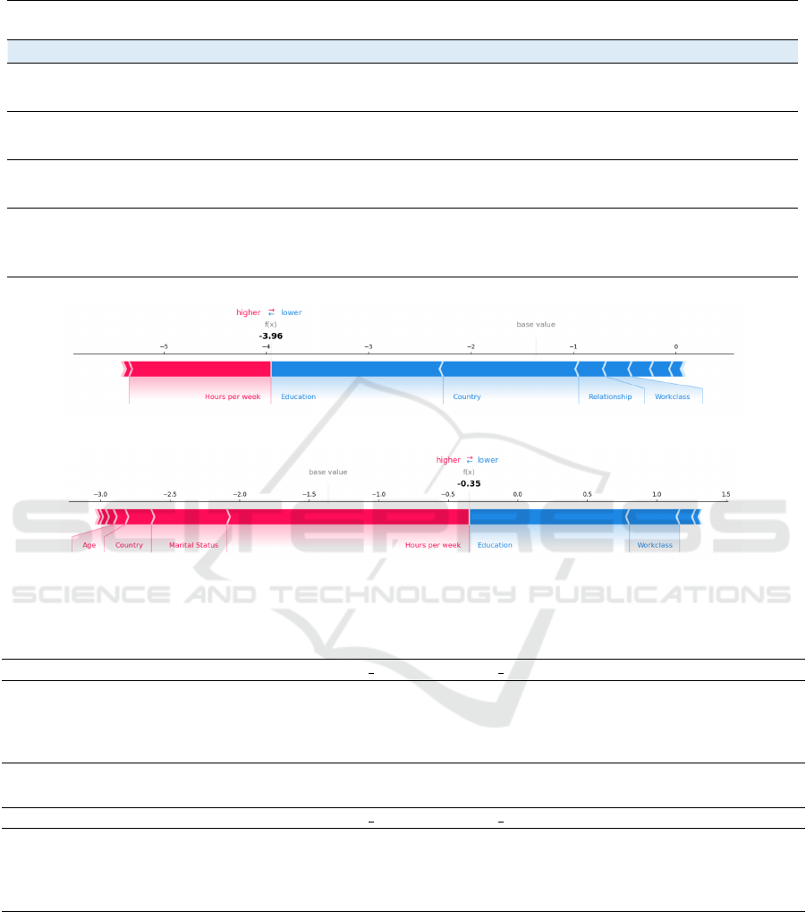
Table 5: An outlier of German Credit and its counterfactuals.
Method
Existing
Checking
Duratio
n
Credit History Purpose
Credit
Amount
Savings
Account
Employment
Since
Installment
Rate
Percentage
Personal
Status Sex
Other
Debtors
Present
Residence
Since
Property Age
Other
Installme
ntPlans
Housing
Existing
Credits
At Bank
Job
People
Liable
ToProvide
Telephone
Foreign
Worker
Original
0-200 DM
42 all paid
car(used)
9283 <100 DM unemploy 1
male:single
none 2 unknown 55 bank free 1
mgmt/self
1 yes yes
- 40 critical - 8597
100-500DM
>=7yrs - - co-app 3 - 44 stores - - skilled - - -
- 41 late pay - 9233
100-500DM
1-3yrs - -
guarantor
- - 43 stores - - unskilled - - -
- - - - 9676
100-500DM
1-3yrs - -
guarantor
3 - 46 stores - - - - - -
- - late pay - 8885
100-500DM
>=7yrs - - co-app 3 realest 42 stores - - unskilled - - -
- 43 paid till - 8746 unknown >=7yrs - - co-app 3 - 54 stores - - unskilled - - -
- - - - 342 - - - - - - - - - - - - - - -
- - - - 342 - - 2 - - - - - - - - - - - -
- 11 - - 9283 - - - - - - - - - - - - - - -
- - critical - 9283 - - - - - 3 - - - - - - - - -
- - - - 6326 - - - - - - - 27 - - - - - - -
- 24 critical - 250 - 1-3yrs - - - - - 34 none own - - - - -
- 15 - - 6850
100-500DM
- - - - - life ins 34 none own - - - - -
noaccount
12 paid till - 7472 - - - - - - car 28 - - - unskilled - - -
- 12 - - 6078
100-500DM
- - - - - car 19 none - -
unemploy
- - -
- 24 late pay - 6403 - >=7yrs - - - - car 34 none - - - - none -
<0 DM 24 paid till - 6579 - - 4 - - - - 29 none - - - - - -
noaccount
24 paid till - 7814 - 4-6yrs 3 - - 3 car 38 none own - - - - -
- 36 paid till - 6948 - 1-3yrs 2 - - - car 35 none rent - - - - -
noaccount
33 critical - 7253 - 4-6yrs 3 - - - car 35 none own 2 - - - -
- 27 late pay - 5965 - >=7yrs - - - - car 30 none own 2 - - - -
Alibi-CFRL
DiCE-Random
DiCE-Genetic
DiCE-KDTree
(a) Centre in Adult Census.
(b) Outlier in Adult Census.
Figure 2: SHAP force plots for the Adult Census dataset.
Table 6: Comparison of different methods on Adult Census.
Method Time(s) Validity Proximity cont Proximity cat Sparsity Constraints Manifold
Alibi-CFRL 0.636 0.965 0.000 0.059 3.125 0.035 8.184
DiCE-Random 0.161 0.760 0.005 0.101 5.355 0.010 1.933
DiCE-Genetic 0.682 0.760 0.049 0.199 10.765 0.000 8.031
DiCE-KDTree 0.410 0.760 0.049 0.201 10.870 0.000 8.000
Table 7: Comparison of different methods on German Credit.
Method Time(s) Validity Proximity cont Proximity cat Sparsity Constraints Manifold
Alibi-CFRL 0.073 1.000 0.000 0.204 2.652 0.913 13.784
DiCE-Random 0.224 1.000 0.028 0.127 1.792 0.761 2.681
DiCE-Genetic 2.609 1.000 0.186 0.841 11.857 0.000 13.429
DiCE-KDTree 1.882 1.000 0.186 0.869 12.236 0.000 13.000
more intricate data patterns, making counterfactual
generation more time-consuming. Additionally, the
increased number of attributes in the German Credit
might lead to higher sparsity and proximity values, as
more features can change in the generated counterfac-
tuals. The differences in the datasets’ nature, distribu-
tion, and inherent relationships likely contribute to the
variations in the metrics observed.
When choosing CFE algorithms in practice, if the
primary focus is constraint satisfaction and time effi-
ciency, Alibi-CFRL is the best choice. It has a param-
eter ranges to set conditions for user-selected vari-
ables that can only be increased or decreased, whereas
conditions in DiCE need to read the value of the in-
stance and manually set the range of values for it.
When inquiring CFEs of a single instance, giving con-
ICAART 2024 - 16th International Conference on Agents and Artificial Intelligence
194

(a) Centre in German Credit.
(b) Outlier in German Credit.
Figure 3: SHAP force plots for the German Credit dataset.
straints is not particularly troublesome. But when in-
quiring CFEs for many instances at once, a succinct
way of setting conditions is worth considering. For
those who value proximity to the original data dis-
tribution, DiCE-Random is likely to be the best all-
rounder.
5.2 Failure of Finding Native CFEs
Viewing the failure of finding valid CFEs by DiCE-
KDTree, relying solely on existing data points can in-
advertently narrow the space of solutions. Existing
data points might not capture the full spectrum of po-
tential counterfactuals, leading to a constrained and
potentially biased view. This bias is further exacer-
bated if the original datasets carry inherent prejudices
based on their collection or curation methodologies.
Another concern is the potential for privacy
breaches. Drawing counterfactuals from existing
datasets might inadvertently expose sensitive or per-
sonal information (Goethals et al., 2023), especially
if the datasets contain confidential data. This risk is
accentuated in today’s data-driven world, where pri-
vacy preservation is paramount. For instance, a link-
age attack is a malevolent effort that involves using
background information to uncover the identity (i.e.,
re-identification) of a concealed entry in a released
dataset (Vo et al., 2023).
On the other hand, although computationally in-
tensive, synthetic CFEs offer a broader, more diverse
exploration of scenarios without the associated pri-
vacy risks. Given these considerations, the inclination
towards synthetic counterfactuals, free from existing
dataset constraints and potential biases, appears pru-
dent for comprehensive and ethical analysis. There-
fore, when designing CFE algorithms, we need to
consider pre-processing the data to ensure privacy and
prevent the original data from being recognized or re-
stored.
5.3 Comparison with Related Work
In our study, the performance of DiCE-KDTree is
found to be the worst among the evaluated algo-
rithms. However, unlike the complete failure to com-
pute metrics as reported in (Verma et al., 2022) for the
Adult Census and German Credit datasets, our evalu-
ation showed that DiCE-KDTree can still output valid
CFEs to a certain extent. Furthermore, while Verma
et al. (2022) evaluated other DiCE algorithms on the
Adult Census and German Credit datasets, they did
not assess Alibi-CFRL. In contrast, Alibi-CFRL has
been reported to exhibit outstanding performance in
validity, sparsity, and manifold distance (Samoilescu
et al., 2021). However, our findings extend this eval-
uation by considering proximity and constraint satis-
faction, which were not addressed in previous papers.
Lastly, even though we used an inverse measurement
of proximity, our conclusion aligns with (Vo et al.,
2023), indicating that DiCE-Random alters fewer fea-
tures compared to DiCE-Genetic.
6 CONCLUSION
6.1 Contributions
In this work, we explored various CFE methods and
compared their properties on the central data points,
the outlier, and the unfavoured class of the dataset,
which is ‘<$ 50k’ in Adult Census and ‘Bad’ in Ger-
man Credit. For data preprocessing, we built an au-
toencoder using Artificial Neural Network to reduce
the feature space. We then applied fine-tuned XG-
Boost for classification, reaching the weighted F1-
score of 0.71 for German Credit and 0.87 for Adult
Census.
We systematically compared DiCE-Random,
DiCE-Genetic, DiCE-KDTree and Alibi-CFRL
Multi-Granular Evaluation of Diverse Counterfactual Explanations
195

across outliers and centres as sample instances in
both datasets and compared their suggested changes
with SHAP force plot. To have a broader insight, we
further tested their time, validity, proximity, sparsity,
constraint satisfaction and manifold distance on the
unfavoured class. To conclude, we discovered
• Features of larger importance by SHAP are not
the ones CFEs suggest to change in most the four
CFE algorithms we evaluated.
• Alibi-CFRL has better performance on proximity
and constraint satisfaction, while DiCE-Random
has better performance on manifold distance. For
datasets with more features, DiCE-Random uses
less time to output the same amount of diverse
CFEs.
• Synthetic CFEs perform better than native CFEs
for data privacy and wider feature ranges because
DiCE-KDTree fails to perform in various metrics.
6.2 Limitations and Future Work
However, our analysis comes with certain limitations
listed as follows. Firstly, in terms of datasets, only
tabular data have been considered. Secondly, our met-
ric for assessing ordinal categorical proximity does
not adequately capture the nuances of real-world sce-
narios. Specifically, while the measure can identify
if a change has occurred, it does not differentiate be-
tween the magnitudes of different changes. For in-
stance, the effort to be made in the real world al-
tering the savings account from ‘unknown’ to ‘500-
1kDM’ is substantially greater than transitioning to
‘<100 DM’. However, in our computations, where we
adopted a simplified approach, these two transitions
are treated as equivalent. This limitation warrants fur-
ther refinement to ensure a more accurate representa-
tion of real-world implications in our analysis.
In future work, we have the following directions.
• Focus on causal constraints: More methods con-
sider actionability as loss terms in the optimizing
problem or reward function in the reinforcement
learning process. Future work can design algo-
rithms and metrics that can capture more causal
constraint patterns. One possible direction is us-
ing Bayes Networks.
• Consider data privacy: Future research could
delve into advanced data preprocessing tech-
niques and the development of algorithms that in-
herently prioritize privacy.
• Conduct user studies: There could also be a pos-
sibility of building an interactive end-to-end XAI
system where we display CFEs and let end-users
decide which method fits them best.
ACKNOWLEDGEMENTS
This work is partially funded by the EPSRC CHAI
project (EP/T026820/1).
REFERENCES
Artelt, A. and Hammer, B. (2021a). Convex optimization
for actionable plausible counterfactual explanations.
arXiv preprint arXiv:2105.07630.
Artelt, A. and Hammer, B. (2021b). Efficient computa-
tion of contrastive explanations. In Proceedings of the
2021 International Joint Conference on Neural Net-
works, pages 1–9. IEEE.
Brughmans, D., Leyman, P., and Martens, D. (2023). Nice:
an algorithm for nearest instance counterfactual ex-
planations. Data Mining and Knowledge Discovery,
pages 1–39.
Chen, T. and Guestrin, C. (2016). Xgboost: A scalable
tree boosting system. In Proceedings of the 22nd
ACM SIGKDD International Conference on Knowl-
edge Discovery and Data Mining, pages 785–794.
Dandl, S., Molnar, C., Binder, M., and Bischl, B. (2020).
Multi-objective counterfactual explanations. In Pro-
ceedings of the 2020 International Conference on Par-
allel Problem Solving from Nature, pages 448–469.
Springer.
De Toni, G., Viappiani, P., Lepri, B., and Passerini, A.
(2022). User-aware algorithmic recourse with pref-
erence elicitation. arXiv preprint arXiv:2205.13743.
F
¨
orster, M., H
¨
uhn, P., Klier, M., and Kluge, K. (2021). Cap-
turing users’ reality: A novel approach to generate co-
herent counterfactual explanations. In Proceedings of
the 54th Hawaii International Conference on System
Sciences, pages 1274–1283.
Goethals, S., S
¨
orensen, K., and Martens, D. (2023). The
privacy issue of counterfactual explanations: explana-
tion linkage attacks. ACM Transactions on Intelligent
Systems and Technology, 14(5):83, 24 pages.
Guidotti, R. (2022). Counterfactual explanations and how to
find them: literature review and benchmarking. Data
Mining and Knowledge Discovery, pages 1–55.
Guidotti, R., Monreale, A., Ruggieri, S., Pedreschi, D.,
Turini, F., and Giannotti, F. (2018). Local rule-based
explanations of black box decision systems. arXiv
preprint arXiv:1805.10820.
Kanamori, K., Takagi, T., Kobayashi, K., and Arimura, H.
(2020). Dace: Distribution-aware counterfactual ex-
planation by mixed-integer linear optimization. In IJ-
CAI, pages 2855–2862.
Karimi, A.-H., Barthe, G., Balle, B., and Valera, I. (2020).
Model-agnostic counterfactual explanations for con-
sequential decisions. In Proceedings of the 2020 In-
ternational Conference on Artificial Intelligence and
Statistics, pages 895–905. PMLR.
Keane, M. T. and Smyth, B. (2020). Good counterfac-
tuals and where to find them: A case-based tech-
nique for generating counterfactuals for explainable ai
ICAART 2024 - 16th International Conference on Agents and Artificial Intelligence
196

(xai). In Case-Based Reasoning Research and Devel-
opment: 28th International Conference, ICCBR 2020,
Salamanca, Spain, June 8–12, 2020, Proceedings 28,
pages 163–178. Springer.
Lash, M. T., Lin, Q., Street, N., Robinson, J. G., and
Ohlmann, J. (2017). Generalized inverse classifica-
tion. In Proceedings of the 2017 SIAM International
Conference on Data Mining, pages 162–170. SIAM.
Le, T., Wang, S., and Lee, D. (2020). Grace: generating
concise and informative contrastive sample to explain
neural network model’s prediction. In Proceedings
of the 26th ACM SIGKDD International Conference
on Knowledge Discovery & Data Mining, pages 238–
248.
Lundberg, S. M. and Lee, S.-I. (2017). A unified approach
to interpreting model predictions. Advances in Neural
Information Processing Systems, 30:4765–4774.
Mahajan, D., Tan, C., and Sharma, A. (2019). Pre-
serving causal constraints in counterfactual explana-
tions for machine learning classifiers. arXiv preprint
arXiv:1912.03277.
Molnar, C. (2022). Interpretable Machine Learning. 2 edi-
tion.
Mothilal, R. K., Sharma, A., and Tan, C. (2020). Explain-
ing machine learning classifiers through diverse coun-
terfactual explanations. In Proceedings of the 2020
Conference on Fairness, Accountability, and Trans-
parency, pages 607–617.
Naumann, P. and Ntoutsi, E. (2021). Consequence-aware
sequential counterfactual generation. In Machine
Learning and Knowledge Discovery in Databases. Re-
search Track: European Conference, ECML PKDD
2021, Bilbao, Spain, September 13–17, 2021, Pro-
ceedings, Part II 21, pages 682–698. Springer.
Pawelczyk, M., Broelemann, K., and Kasneci, G. (2020).
Learning model-agnostic counterfactual explanations
for tabular data. In Proceedings of the Web Conference
2020, pages 3126–3132.
Poyiadzi, R., Sokol, K., Santos-Rodriguez, R., De Bie, T.,
and Flach, P. (2020). Face: feasible and actionable
counterfactual explanations. In Proceedings of the
2020 AAAI/ACM Conference on AI, Ethics, and So-
ciety, pages 344–350.
Ribeiro, M. T., Singh, S., and Guestrin, C. (2016). ” why
should i trust you?” explaining the predictions of any
classifier. In Proceedings of the 22nd ACM SIGKDD
International Conference on Knowledge Discovery
and Data Mining, pages 1135–1144.
Samoilescu, R.-F., Van Looveren, A., and Klaise, J. (2021).
Model-agnostic and scalable counterfactual explana-
tions via reinforcement learning. arXiv preprint
arXiv:2106.02597.
Schleich, M., Geng, Z., Zhang, Y., and Suciu, D. (2021).
Geco: Quality counterfactual explanations in real
time. arXiv preprint arXiv:2101.01292.
Schut, L., Key, O., Mc Grath, R., Costabello, L., Sacaleanu,
B., Gal, Y., et al. (2021). Generating interpretable
counterfactual explanations by implicit minimisation
of epistemic and aleatoric uncertainties. In Proceed-
ings of the 2021 International Conference on Artificial
Intelligence and Statistics, pages 1756–1764. PMLR.
Sharma, S., Henderson, J., and Ghosh, J. (2019). Certi-
fai: Counterfactual explanations for robustness, trans-
parency, interpretability, and fairness of artificial in-
telligence models. arXiv preprint arXiv:1905.07857.
Van Looveren, A. and Klaise, J. (2021). Interpretable
counterfactual explanations guided by prototypes. In
Proceedings of the 2021 Joint European Conference
on Machine Learning and Knowledge Discovery in
Databases, pages 650–665. Springer.
Van Looveren, A., Klaise, J., Vacanti, G., and Cobb, O.
(2021). Conditional generative models for counterfac-
tual explanations. arXiv preprint arXiv:2101.10123.
Verma, S., Boonsanong, V., Hoang, M., Hines, K. E., Dick-
erson, J. P., and Shah, C. (2020). Counterfactual
explanations and algorithmic recourses for machine
learning: A review. arXiv preprint arXiv:2010.10596.
Verma, S., Hines, K., and Dickerson, J. P. (2022). Amor-
tized generation of sequential algorithmic recourses
for black-box models. In Proceedings of the AAAI
Conference on Artificial Intelligence, volume 36,
pages 8512–8519.
Vo, V., Le, T., Nguyen, V., Zhao, H., Bonilla, E. V., Haffari,
G., and Phung, D. (2023). Feature-based learning for
diverse and privacy-preserving counterfactual expla-
nations. In Proceedings of the 29th ACM SIGKDD
Conference on Knowledge Discovery and Data Min-
ing, pages 2211––2222. ACM.
Wachter, S., Mittelstadt, B., and Russell, C. (2017). Coun-
terfactual explanations without opening the black box:
Automated decisions and the gdpr. Harvard Journal
of Law & Technology, 31:841.
Multi-Granular Evaluation of Diverse Counterfactual Explanations
197
