Benchmarking Quantum Surrogate Models on Scarce and Noisy Data
Jonas Stein
1
, Michael Poppel
1
, Philip Adamczyk
1
, Ramona Fabry
1
, Zixin Wu
1
,
Michael K
¨
olle
1
, Jonas N
¨
ußlein
1
, Dani
¨
elle Schuman
1
, Philipp Altmann
1
,
Thomas Ehmer
2
, Vijay Narasimhan
3
and Claudia Linnhoff-Popien
1
1
LMU Munich, Germany
2
Merck KGaA, Darmstadt, Germany
3
EMD Electronics, San Jose, California, U.S.A.
fi
Keywords:
Quantum Computing, Surrogate Model, NISQ, QNN.
Abstract:
Surrogate models are ubiquitously used in industry and academia to efficiently approximate black box func-
tions. As state-of-the-art methods from classical machine learning frequently struggle to solve this problem
accurately for the often scarce and noisy data sets in practical applications, investigating novel approaches is
of great interest. Motivated by recent theoretical results indicating that quantum neural networks (QNNs) have
the potential to outperform their classical analogs in the presence of scarce and noisy data, we benchmark their
qualitative performance for this scenario empirically. Our contribution displays the first application-centered
approach of using QNNs as surrogate models on higher dimensional, real world data. When compared to a
classical artificial neural network with a similar number of parameters, our QNN demonstrates significantly
better results for noisy and scarce data, and thus motivates future work to explore this potential quantum ad-
vantage. Finally, we demonstrate the performance of current NISQ hardware experimentally and estimate the
gate fidelities necessary to replicate our simulation results.
1 INTRODUCTION
The development of new products in industrial in-
novation cycles can take dozens of years with R&D
costs ranging up to several billion dollars. At the cen-
ter of such processes (which are ubiquitous to, e.g.,
materials, financial and chemical industries) lies the
problem of identifying the outcome of an experiment,
given a specific input (Batra et al., 2021; Cizeau et al.,
2001; McBride and Sundmacher, 2019). Having to
account for highly complex interactions in the ex-
amined elements typically demands for tedious real-
world experiments, as computational simulations ei-
ther have very long runtimes or approximate the ac-
tual outcomes insufficiently. As a result, only a small
number of configurations can be tested in each prod-
uct development iteration, often leading to suboptimal
and misguided steps. Additionally, experiments suf-
fer from aleatoric uncertainty, i.e., imprecisions in the
experiment set-up, read-out errors, or other types of
noise.
A popular in silico approach for accelerating such
simulations are so called surrogate models, which aim
to closely approximate the simulation model while
being much cheaper to evaluate. Their central tar-
get is fitting a computational model to the available
data. More recently, the usage of highly parameter-
ized models like classical Artificial Neural Networks
(ANNs) as surrogate models has gained increasing re-
search interest, as they have shown promising perfor-
mance in coping with the typically high dimensional
solution space (Sun and Wang, 2019; Qin et al., 2022;
Vazquez-Canteli et al., 2019). However, a substantial
issue with using ANNs as surrogate models is over-
fitting, which is mainly caused by a combination of
noisiness and small sample sizes of the available data
points in practice. (Stokes et al., 2020; Ma et al.,
2015; Gawehn et al., 2016)
In contrast to classical ANNs, quantum neural net-
works (QNNs), have been shown to be quite robust
with respect to noise and data scarcity (Peters and
Schuld, 2023; Mitarai et al., 2018). Furthermore,
QNNs also natively allow to efficiently process data in
higher dimensions than classically possible, display-
ing another possible quantum advantage.
Eager to investigate the usage of QNNs as surro-
gate models in a realistic setting (i.e., given a limited
number of noisy data points), our core contributions
352
Stein, J., Poppel, M., Adamczyk, P., Fabry, R., Wu, Z., Kölle, M., Nüßlein, J., Schuman, D., Altmann, P., Ehmer, T., Narasimhan, V. and Linnhoff-Popien, C.
Benchmarking Quantum Surrogate Models on Scarce and Noisy Data.
DOI: 10.5220/0012348900003636
Paper published under CC license (CC BY-NC-ND 4.0)
In Proceedings of the 16th International Conference on Agents and Artificial Intelligence (ICAART 2024) - Volume 3, pages 352-359
ISBN: 978-989-758-680-4; ISSN: 2184-433X
Proceedings Copyright © 2024 by SCITEPRESS – Science and Technology Publications, Lda.

amount to:
• An exploration of the practical application of
QNNs as surrogate functions beyond existing
proofs of concept, i.e., by fitting scarce, noisy,
data sets in higher dimensions.
• An extensive evaluation of the designed QNNs
against a similarly sized ANN, constructed to
solve the given tasks accurately when given many
noise free data samples.
• An empirical analysis of NISQ hardware perfor-
mance and an estimation of needed hardware error
improvements to replicate the simulator results.
2 BACKGROUND
A surrogate function g is typically used to approxi-
mate a given black box function f for which some
data points ((x
1
, f (x
1
)),...,(x
n
, f (x
n
))) are given, or
can be obtained from a costly evaluation of f . The
goal in surrogate modelling is finding a suitable, effi-
cient whitebox function g such that
d ( f (x
i
),g(x
i
)) ≤ ε (1)
where d denotes a suitable distance metric and ε > 0
is sufficiently small for all x
i
. Possible employed
functions and techniques for representing g include
polynomials, Gaussian Processes, radial basis func-
tions and classical ANNs (McBride and Sundmacher,
2019; Queipo et al., 2005; Khuri and Mukhopadhyay,
2010).
In our approach, we use a QNN, which modifies
the parameters θ of a parameterized quantum circuit
(PQC) to approximate the function f as described in
(Mitarai et al., 2018). Each input data sample x
i
is
initially encoded into a quantum state
|
ψ
in
(x
i
)
⟩
and
then manipulated by a series of unitary quantum gates
of a PQC U(θ,x).
|
ψ
out
(x
i
,θ)
⟩
= U(θ,x)
|
ψ
in
(x
i
)
⟩
(2)
Choosing a suitable measurement operator M
(e.g., the Pauli Z-operator for each qubit σ
z
i
), the ex-
pectation value gets measured to obtain the predicted
output data.
g
QNN
(x
i
) =
⟨
ψ
out
(x
i
,θ)
|
M
|
ψ
out
(x
i
,θ)
⟩
(3)
Aggregating the deviation of the generated output
from the original output data then provides a quan-
tification of the quality of the prediction which will
finally be used to update the parameters of the gates
within the PQC in the next iteration.
To encode the provided input data sample, many
possibilities such as basis encoding, angle encoding
and amplitude encoding have been explored in liter-
ature (Weigold et al., 2021). While some of these
encodings, typically called feature maps, exploit the
richer tool set available in quantum computing to very
efficiently upload more than one classical data point
into one qubit (e.g., amplitude encoding), others trade
off the dense encoding for faster state preparation
(e.g., angle encoding).
For the PQC, typically called ansatz, many archi-
tectures have been proposed. These generally consist
of parameterized single qubit rotation and entangle-
ment layers. (Sim et al., 2019) provides an overview
of various circuit architectures, together with their ex-
pressibility and entangling capability. In this context,
expressibility describes the size of the subset of states
that can be reached from a given input state by chang-
ing the parameters of the ansatz. The more states can
be reached, the more universal the quantum function
can be.
As shown in (Schuld et al., 2021a), quantum mod-
els can be written as partial Fourier series in the data,
which can in turn represent universal function approx-
imators for a rich enough frequency spectrum. Fol-
lowing this, techniques like parallel encoding, as well
as data reuploading display potent tools in modelling
more expressive QNNs (Schuld et al., 2021a; P
´
erez-
Salinas et al., 2020). More specifically, parallel en-
coding describes the usage of a quantum feature map
in parallel, i.e., for multiple qubit registers at the same
time, while data reuploading is defined as the repeated
application of the feature map throughout the circuit.
The approximation quality achieved by the QNN
(i.e., ε from equation 1) can be quantified by choosing
a suitable distance function, such as the mean squared
error. Employing a suitable parameter optimization
method such as the parameter shift rule allows for
training the QNN’s parameters. Notably, all known
gradient-based techniques for parameter optimization
(such as the parameter shift rule) scale linearly in their
runtime with respect to the number of parameters,
limiting the number of parameters, that can be trained
given a limited amount of time compared to classical
backpropagation. (Mitarai et al., 2018)
3 METHODOLOGY
To benchmark the practical application of QNNs
as surrogate functions, we propose the following
straightforward procedure: (1) Identify suitable QNN
architectures, (2) select a realistic data set and (3)
choose a reasonable classical ANN as baseline.
Benchmarking Quantum Surrogate Models on Scarce and Noisy Data
353

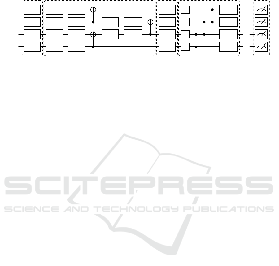
FM CIRCUIT 11 FM CIRCUIT 9 MSMT
...
...
...
...
|
0
⟩
R
x
(x
0
)
R
y
(θ
0
)
R
z
(θ
4
) R
x
(x
0
)
H
R
x
(θ
12
)
|
0
⟩
R
x
(x
1
)
R
y
(θ
1
)
R
z
(θ
5
)
R
y
(θ
8
)
R
z
(θ
10
) R
x
(x
1
)
H
R
x
(θ
13
)
|
0
⟩
R
x
(x
0
)
R
y
(θ
2
)
R
z
(θ
6
)
R
y
(θ
9
)
R
z
(θ
11
) R
x
(x
0
)
H
R
x
(θ
14
)
|
0
⟩
R
x
(x
1
)
R
y
(θ
3
)
R
z
(θ
7
) R
x
(x
1
)
H
R
x
(θ
15
)
Figure 1: The general QNN architecture used in this paper, exemplarily showing two layers, each comprised of a data encoding
and a parameterized layer. It combines data reuploading by inserting a feature map (“FM”) in each layer with parallel encoding
by using two qubits per input data point dimension. For the parameterized part of the circuit, two different circuits from
established literature have been combined: Circuit 11 is alternating with circuit 9 to create the required minimum number
of parameters (Sim et al., 2019). CNOT, Hadamard and CZ gates create superposition and entanglement, while trainable
parameters θ
i
allow the approximation of the surrogate model. After repeated layers, the standard measurement (denoted with
“MSMT”) is applied to all qubits.
3.1 Identifying Suitable Ans
¨
atze
Following the description of all QNN components in
section 2, we now (1) identify a suitable encoding,
(2) select an efficient ansatz for the parameterized cir-
cuit, then (3) combine both using layering and finally
(4) choose an appropriate decoding of measurement
results to represent the prediction result.
Paying tribute to the limited hardware capabilities
of current NISQ hardware, we employ angle encod-
ing and hence focus on small- to medium-dimensional
data sets. In particular, angle encoding has the use-
ful property of generating desired expressibility while
keeping the required number of gates and parameters
low, resulting in shallower, wider circuits compared to
more space-efficient encodings such as amplitude en-
coding (Ostaszewski et al., 2021; Mantri et al., 2017).
A possible implementation can be seen in the first two
wires of figure 1, where two-dimensional input data
x = (x
0
,x
1
) is angle encoded using R
x
rotations.
For selecting an efficient ansatz, we use estab-
lished circuits proposed in literature (Sim et al.,
2019), that allow for a high degree of expressibil-
ity and entanglement capacity to harness the essential
tools allowing for quantum advantage. An important
feature of these ans
¨
atze is, that they underlie an in-
trinsic structure, which allows scaling their width to
fit an arbitrary number of qubits. Furthermore, we
acknowledge a core result of ansatz design, i.e., the
number of parameters in the ansatz should at least be
twice the number of data encodings in the entire cir-
cuit to fully exploit the spectrum of the necessary non-
linear effects generated by data reuploading and par-
allel encoding (Schuld et al., 2021a). Targeting our
circuit choice towards an optimal trade-off between
high expressibility and a low number of parameters
(while adhering to the above mentioned lower bound),
we use a combination of the two most expressive cir-
cuits from (Sim et al., 2019), i.e., “circuit 9” and “cir-
cuit 11”, as their concatenation perfectly matches the
lower bound of parameters. For details, see figure 1.
Apart from the employed layered circuit architec-
ture, we also employ parallel encoding and data reu-
ploading to allow building a sufficient quantum func-
tion approximator, in-line with (Schuld et al., 2021a)
and most PQCs employed in literature. While data
reuploading and parallel encoding both have a simi-
lar effect on expressibility (P
´
erez-Salinas et al., 2020;
Schuld et al., 2021b; Schuld and Petruccione, 2021),
in preliminary experiments conducted for this paper
data reuploading appeared to be more effective than
parallel encoding, as it led to faster evaluations with
higher R2 scores for our data sets. Additional em-
pirical results led to the final circuit architecture dis-
played in figure 1, where a small amount of parallel
encoding was applied (i.e., only once), while the fo-
cus is on data reuploading. In practice, empirical data
shows, that the number of necessary layers can vary
from data set to data set by a lot (in our cases, from 6
layers up to 42 layers), for details, see section 4.
After the various data encoding and parameter-
ized layers in the QNN, a measurement operator is
mandatory to extract classical information from the
circuit. Having tried various different possibilities
(tensor products of σ
z
and I matrices), preliminary
studies to this work led to the selection of the stan-
dard measurement operator σ
z
for all qubits involved.
Note that this demands for a suitable rescaling of the
output values if the image of the function to be fit-
ted lives outside the interval [−1,1] (which typically
is a parameter that can be estimated by domain ex-
perts in the given use case). The difference between
the obtained output and the original data is calculated
as the mean squared error, and the parameters θ for
the next iteration are generated with the help of an
optimizer. Following the optimizer benchmark study
ICAART 2024 - 16th International Conference on Agents and Artificial Intelligence
354

results provided in (Joshi et al., 2021; Huang et al.,
2020), COBYLA (Gomez et al., 1994) was chosen for
this purpose.
3.2 Selecting Benchmark Data Sets
In previous work, (Mitarai et al., 2018) and (Qiskit
contributors, 2023) showed that QNNs can fit very
simple functions with one-dimensional input like
sin(x), x
2
or e
x
. To go beyond these proofs of concept,
we explore the following, more complex, standard, d-
dimensional functions regularly used for benchmark-
ing data fitting:
• Griewank func.
∑
d
i=1
x
2
i
/4000 −
∏
d
i=1
cos(
x
i
/
√
i) + 1
for x ∈[−5, 5]
d
(Griewank, 1981)
• Schwefel func. 418.9829d −
∑
d
i=1
x
i
sin

p
|
x
i
|

for x ∈[−50, 50]
d
(Schwefel, 1981)
• Styblinski-Tang func.
1
/2
∑
d
i=1

x
4
i
−16x
2
i
+ 5x
i

for x ∈[−5, 5]
d
(Styblinski and Tang, 1990)
For each of these benchmark functions, we used two-
dimensional input data, which, together with the one-
dimensional function value, can still be presented in
three-dimensional surface plots. In addition to that,
we also investigate the performance on the real world
data set Color bob (H
¨
ase et al., 2021), which con-
tains 241 six-dimensional data points from a chemi-
cal process related to colorimetry. The intervals of the
functions are chosen to balance complexity and visual
observability, while keeping the number of required
parameters in the PQC at a level that still allows for
the necessary iterative calculations within reasonable
time (i.e., a couple of days on our hardware). To fa-
cilitate an unambiguous angle encoding (for details,
see (K
¨
olle. et al., 2023)), we normalize the data to the
range [0,1] in all dimensions.
3.3 Selecting a Classical Baseline
As classical machine learning is tremendously better
understood and currently far more performant than
quantum machine learning, it is strongly to be as-
sumed, that ANNs can be identified, that achieve
(near) perfect results in all of our experiments, as the
datasets are comparably small and simple. Aiming
to provide a meaningful comparison nevertheless, we
take a standard approach of choosing a similarly sized
ANN as baseline, i.e., in terms of the number of pa-
rameters. Preliminary studies conducted for this arti-
cle show, that already quite small ANNs can achieve
accurate fits, i.e., a fully connected feedforward neu-
ral network consisting of an input layer (with as many
neurons as dimensions in the domain space of the
function), two hidden layers (containing 7 neurons
and using a sigmoid activation function) and an out-
put layer of size one. While the in- and output layers
are fixed in size by the datasets used, the number of
n = 7 neurons per hidden layer is an empirical result
obtained by iteratively increasing n, until the R2 score
exceeded 90% for every dataset. This amounts to 140
parameters, which corresponds to a QNN comprised
of 9 layers of the employed architecture (as displayed
in figure 1). As no regularization technique was ap-
plied for the QNN, none is used for the ANN either, in
order to compare the two models on a like-for-like ba-
sis. Analog to the QNN, we employ the mean squared
error loss. For parameter training, we use the popular
ADAM optimizer (Kingma and Ba, 2014) and train
for 50,000 optimization steps.
4 EVALUATION
Having prepared a suitable QNN architecture, a clas-
sical ANN as baseline and a variety of challenging
benchmark functions, we now evaluate the applica-
bility of QNNs as surrogate functions in domains
with scarce and noisy data. For all experiments, a
80/20 train/test split was used, and all displayed re-
sults show the performance on the test data.
4.1 Baseline Results for Noiseless Data
To quantify our results, we use the R2 score, a stan-
dard tool to measure the similarity of estimated func-
tion values to the original data point values, as well as
visual inspection, to assess how well the shape of the
original function gets approximated. The R2 score
is defined such that it yields one if the model per-
fectly predicts the outcome, and lower values, the less
well it predicts the outcome (where random guessing
amounts to an R2 score of 0):
R2(y, ˆy) = 1 −
n
∑
i=1
(y
i
− ˆy
i
)
2
n
∑
i=1
(y
i
− ¯y
i
)
2
(4)
Here, n is the number of given samples, y
i
is the origi-
nal value, ˆy
i
is the predicted value and ¯y
i
=
1
/n
∑
n
i=1
y
i
.
For all benchmark functions with two-
dimensional input data mentioned in section 3.2, the
QNN achieves very good R2 scores, even obtaining
values above 0.9, when given the ”full dataset” (i.e.,
an evenly spaced 50-by-50 grid of 2500 noiseless
data points, as described in section 4.2). To achieve
this solution quality, we identify a minimum of 20
(42) layers and 3000 (4000) optimization iterations
Benchmarking Quantum Surrogate Models on Scarce and Noisy Data
355

0.0
0.2
0.4
0.6
0.8
1.0
0.0
0.2
0.4
0.6
0.8
1.0
0.0
0.2
0.4
0.6
0.8
1.0
(a) Original Schwefel func-
tion surface.
0.0
0.2
0.4
0.6
0.8
1.0
0.0
0.2
0.4
0.6
0.8
1.0
0.1
0.2
0.3
0.4
0.5
0.6
0.7
0.8
(b) QNN generated surface,
R2 score of 0.94.
Figure 2: Qualitative performance of the quantum surrogate
for the Schwefel function with two-dimensional input.
required for the Griewank (Schwefel and Styblinski-
Tang) functions. Exemplary results of the original
surface and the surrogate model surface for the
two-dimensional Schwefel function are displayed in
figure 2. For the Color bob data set, we obtain an
R2 score close to 0.9 with 3 layers consisting only
of the feature map and ansatz 1 from figure 1, with
merely 500 optimization iterations given the full
dataset. To account for the increased dimensionality
in the input data, we used five qubits, and skipped
the parallel encoding, as the results turned out to be
good enough without it. This demonstrates the first
evidence towards promising performance of quantum
surrogate models on industrially relevant, real world,
dataset for very minor hardware requirements.
4.2 Introducing Noise and Data Scarcity
In real world applications, the available data samples
are often scarce and noisy. In order to model this situ-
ation, we introduce different degrees of noise on vary-
ing training set sizes. For this rather time intensive
part of the evaluation, we focus on the Griewank func-
tion, as the number of layers and iterations (i.e., the
computational effort) required to find a suitable quan-
tum surrogate model for this function is a lot lower
than for the others.
Given the discussed QNN (see figure 1) and clas-
sical ANN (see section 3.3), we evaluate them for a
range of 100, 400, 900, 1600 and 2500 data points (se-
lected analog to selecting data points in grid search)
while also introducing standard Gaussian noise fac-
tors (Truax, 1980) of 0.1, 0.2, 0.3, 0.4 and 0.5 on the
input data. More specifically, the noise is applied us-
ing the following map (x
i
, f (x
i
)) 7→ (x
i
, f (x
i
) + δν),
where δ denotes the noise factor and ν is random
value sampled from a Gaussian standard normal dis-
tribution ϕ(z) =
exp
(
−z
2
/2
)
/
√
2π. Adding noise on the
input data can therefore be thought of as an impre-
cise black box function execution (e.g., due to inexact
measurements in chemical experiments). For simplic-
0.1 0.2 0.3 0.4 0.5
Noise level
5040302010
Sample size
-0.06 -0.04 -0.02 0.03 0.1
-0.07 -0.07 0.02 0.03 0.05
-0.04 0 0.06 0.07
0.15
-0.02 0 0.06 0.09 0.13
-0.04 -0.01 0.04 0.07 0.06
−0.20
−0.15
−0.10
−0.05
0.00
0.05
0.10
0.15
0.20
Figure 3: Delta R2 score obtained by subtracting the clas-
sical ANN R2 score from the QNN R2 score for differ-
ent noise levels (x-axis) and sample sizes (y-axis) for the
Griewank function with two-dimensional input data. Pos-
itive values indicate a performance advantage of the QNN
(as can be seen for higher noise levels and smaller sample
sizes), while negative values represent a disadvantage of the
QNN.
ity, we use the term sample size in the following to
denote the granularity of the grid in both dimensions,
i.e., we investigate sample sizes of 10, 20, 30, 40, and
50.
As we are mainly interested in the relative per-
formance of the QNN and ANN against each other,
we focus our evaluation on the difference of their R2
scores Delta R2 = R2
QNN
(y, ˆy) −R2
ANN
(y, ˆy), as de-
picted in figure 3. The results show that our QNN
has a tendency to achieve better R2 scores for higher
noise levels compared to the classical ANN. This
trend seems to be even more obvious for smaller sam-
ple sizes compared to larger ones. This indicates, that
QNNs can have better generalization learning ability
when given scarce and noisy data.
In order to also examine the results generated by
the QNN and the classical ANN visually, we depict
plots of the surrogate model for the Griewank func-
tion as well as the original Griewank function and the
function resulting from overlaying noise with a factor
of 0.5 in figure 4. The QNN shows more resilience
than the ANN for increasing noise levels and clearly
maintains the shape of the original function a lot bet-
ter. Notably, for noise levels below 0.3, the classi-
cal ANN was able to achieve higher R2 scores than
the QNN. However, overall, the better performance
of QNN for noisy and scarce data points towards its
comparatively better generalization capabilities.
4.3 NISQ Hardware Results
Today’s HPC quantum circuit simulators have shown
the capability to simulate small circuits up to 60
ICAART 2024 - 16th International Conference on Agents and Artificial Intelligence
356

(a) 3-D Griewank surface.
(b) Noisy surface.
(c) Surface-fit of the QNN. (d) Surface-fit of the ANN.
Figure 4: Surface plots of the Griewank function when
introducing noise and sample scarcity. The input to the
QNN and classical ANN was modified by multiplication of
standard-normal noise with a factor of 0.5 on the 400 in-
dividual input data points (which corresponds to a sample
size of 20).
qubits (Lowe et al., 2023). Taking this as an approx-
imate bound for how many qubits a circuit can con-
sist of in analytic calculations, it becomes apparent,
that classical simulations face a clear limit when as-
sessing high dimensional input data when using qubit
intensive data encoding. Based on our experiments,
two to three qubits per dimension showed the best re-
sults. For a small scale data set with industrial rele-
vance, e.g., the 29-dimensional input data as available
in PharmKG, a project of the pharmaceutical indus-
try (Bonner et al., 2022), this already would require
roughly 87 qubits, thus quickly exceeding what is effi-
ciently possible with classical computers. Therefore,
one needs to rely on quantum hardware in order to
examine scaling performance for higher dimensional
data sets, optimally using fault tolerant qubits.
In order to explore such possibilities, we now test
our quantum surrogate model on an existing quantum
computer. For this, we choose the five qubit QPU
ibmq belem, as it offers sufficient resources for run-
ning our circuits, i.e., availability, number of qubits
and gate fidelities. Despite privileged access and
using the Qiskit Runtime environment (which does
not require re-queuing for each optimization itera-
tion), our multi-layer approach faced difficulties for
all higher dimensional functions. However, after a
manual hyperparameter search, we were able to ob-
tain a fit for the one-dimensional Griewank function
with three qubits, six layers and 100 optimization iter-
ations (executed on the QPU) as depicted in figure 5.
While the achieved R2 score of 0.54 is fairly moder-
ate, we observe that in both evaluations (see figure 4
and 5), the QNN is very accurate in determining the
shape of the underlying function. This can already be
valuable information in practice, as it allows for dis-
cerning desirable from undesirable regions.
4.4 Scaling Analysis
Neglecting decoherence, there are three main types
of errors on real hardware causing failures: Single-
and two-qubit gate errors and readout errors. For the
ibmq belem, the mean Pauli-X error is around 0.04%,
the mean CNOT error roughly amounts to 1.08% and
the readout error is about 2.17%. Taking the mean
Pauli-X error as proxy for single-qubit errors and the
mean CNOT error as proxy for two-qubit gate errors,
one can approximate the probability of a circuit re-
maining without error. Subtracting the error rate from
one results in the “survival rate” per gate, which will
then be exponentiated with the number of respective
gates in the circuit. Our three-qubit, six-layer circuit
for the ibmq belem consists of 10 single-qubit and
two two-qubit gates per layer and three readouts, re-
sulting in a total survival rate of 80.13% for six layers.
The survival rates for different circuit sizes with re-
gard to the number of qubits and the number of layers
is shown in table 1.
Taking this total survival rate of 80.13% as the
minimum requirement for a successful real hardware
run, one can also approximate the required error rate
improvement such that the four-qubit, 20 layer cir-
cuit we use for finding a surrogate model for the
Griewank function with two-dimensional input data
could be run on real hardware. In order to have only
one variable to solve for, we keep the single-qubit er-
ror constant at its current rate and assume that the ra-
tio of readout error to two-qubit gate error remains at
two. This results in a required two-qubit gate error of
0.15% and a readout error of 0.3%, resembling a re-
duction to about 14% of current error levels. Looking
towards more recent IBM QPUs like the Falcon r5.11,
lower error rates than the here employed ibmq belem
are already available: 0.9% for CNOTs and 0.02%
for Pauli-X gates. For this QPU, our calculations
yield a survival rate of 52.76%, which displays sig-
nificant improvement, but still prevents modelling the
Griewank function sufficiently well.
Note, that this analysis does assume, that the train-
ing is executed in a noise-aware manner, i.e., each cir-
cuit execution during the training should be repeated
multiple times to ensure identifying an error free re-
Benchmarking Quantum Surrogate Models on Scarce and Noisy Data
357

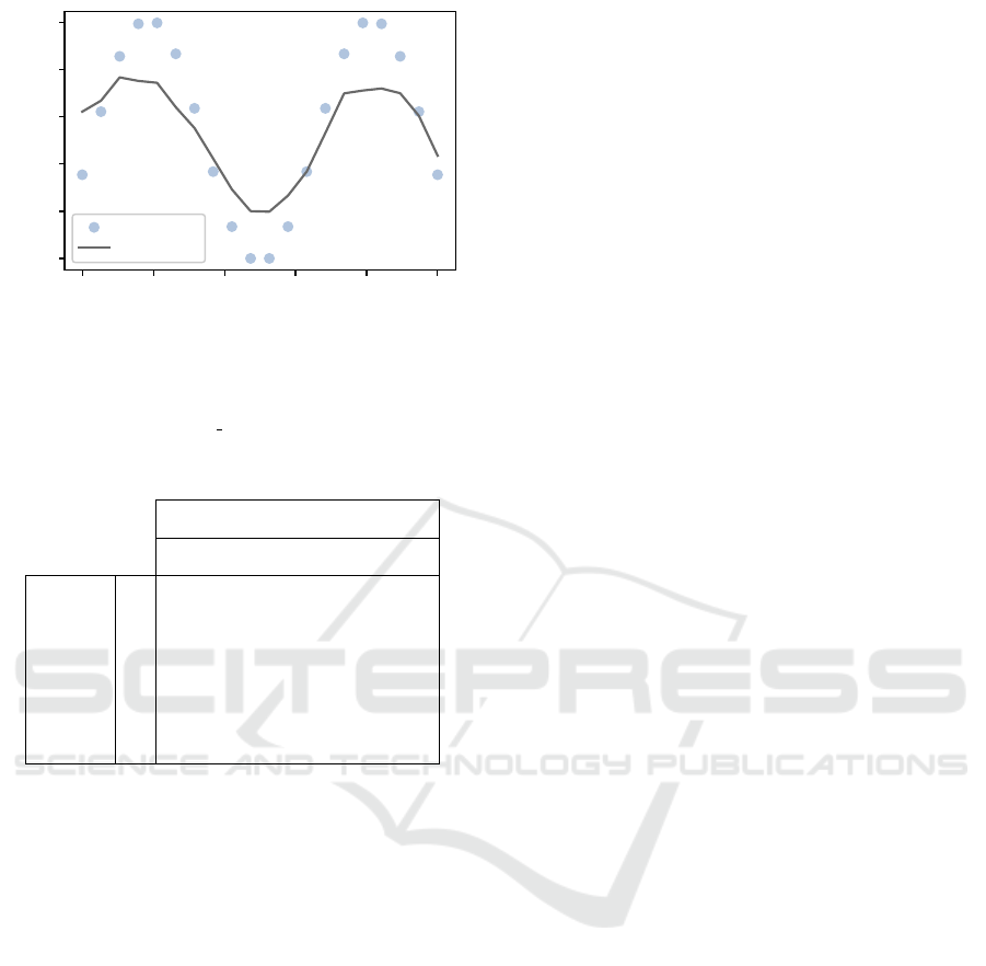
0.0 0.2 0.4 0.6 0.8 1.0
Input value
0.0
0.2
0.4
0.6
0.8
1.0
Output value
data points
fitted
Figure 5: Original data points (sample size of 20) for the
Griewank function with one-dimensional input data and the
quantum surrogate function that has been obtained by run-
ning 100 optimization iterations on our ansatz (see figure 1)
with six layers on the ibmq belem QPU.
Table 1: Estimated survival rates on noisy QPUs.
Number of layers
4 8 12 16 20
Number
of
qubits
2 0.91 0.86 0.82 0.77 0.73
4 0.79 0.67 0.58 0.49 0.42
8 0.59 0.41 0.29 0.20 0.14
16 0.33 0.16 0.07 0.03 0.02
32 0.10 0.02 0.00 0.00 0.00
sult by employing a suitable postprocessing routine.
As the here-demanded success probability of ∼80%
is already quite high, this ensures a negligibly small,
constant, overhead in computation time.
5 CONCLUSION
Surrogate models have provided enormous cost and
time savings in industrial development processes.
Nevertheless, dealing with small and noisy data sets
still remains a challenge, mostly due to overfitting
tendencies of the current state of the art machine
learning approaches applied. In this paper, we have
demonstrated that quantum surrogate models based
on QNNs can offer an advantage over similarly sized
classical ANNs in terms of prediction accuracy for
substantially more difficult data sets than those used
in previous literature, when the sample size is scarce
and substantial noise is present. For this, we con-
structed suitable QNNs, while having employed state-
of-the-art ansatz design knowledge, namely: data pre-
processing in form of scaling, data reuploading, par-
allel encoding, layering with a sufficient number of
parameters and using different ans
¨
atze in one circuit.
In addition to that, our noise and scaling analy-
ses on quantum surrogate models for higher dimen-
sional inputs, combined with the envisaged reduction
of quantum error rates by quantum hardware manu-
facturers show that our simulation results could be
replicated on QPUs in the near future. A possible way
to accelerate this process might be switching from a
data-reuploading-heavy circuit to one focused on par-
allel encoding, as this would shorten the overall cir-
cuit, allowing for the use of more qubits.
In essence, our contribution provides significant
empirical evidence supporting the theoretical claims
of quantum robustness in regards to data scarcity and
input noise. However, due to the small scale of the
conducted case study, the stated implications must
be evaluated on larger real world datasets, for which
classical approaches are infeasible. We expect the
needed refinements to the here employed quantum ap-
proach to mostly depend on a more sophisticated, pos-
sibly automatized, quantum architecture search.
Finally, we encourage future work to expand the
here indicated trade-off between the solution quality
and the number of parameters to also include an anal-
ysis of the runtime. This will be especially interest-
ing for increasingly challenging datasets, as current
NISQ-restrictions only allow for the exploration of
problem instances, that can rapidly be solved by naive
classical approaches.
ACKNOWLEDGEMENTS
This paper was partially funded by the German Fed-
eral Ministry for Economic Affairs and Climate Ac-
tion through the funding program ”Quantum Comput-
ing – Applications for the industry” based on the al-
lowance ”Development of digital technologies” (con-
tract number: 01MQ22008A). Furthermore, this re-
search is part of the Munich Quantum Valley, which
is supported by the Bavarian state government with
funds from the Hightech Agenda Bayern Plus.
REFERENCES
Batra, R., Song, L., and Ramprasad, R. (2021). Emerging
materials intelligence ecosystems propelled by ma-
chine learning. Nature Reviews Materials, 6(8):655–
678.
Bonner, S., Barrett, I. P., Ye, C., Swiers, R., Engkvist, O.,
Bender, A., Hoyt, C. T., and Hamilton, W. L. (2022).
A review of biomedical datasets relating to drug dis-
ICAART 2024 - 16th International Conference on Agents and Artificial Intelligence
358

covery: a knowledge graph perspective. Briefings in
Bioinformatics, 23(6). bbac404.
Cizeau, P., Potters, M., and Bouchaud, J.-P. (2001). Corre-
lation structure of extreme stock returns. Quantitative
Finance, 1(2):217–222.
Gawehn, E., Hiss, J. A., and Schneider, G. (2016). Deep
learning in drug discovery. Molecular Informatics,
35(1):3–14.
Gomez, S., Hennart, J.-P., and Powell, M. J. D., editors
(1994). A Direct Search Optimization Method That
Models the Objective and Constraint Functions by
Linear Interpolation, pages 51–67. Springer Nether-
lands, Dordrecht.
Griewank, A. O. (1981). Generalized descent for global
optimization. J. Optim. Theory Appl., 34(1):11–39.
Huang, Y., Lei, H., and Li, X. (2020). An empirical study
of optimizers for quantum machine learning. In 2020
IEEE 6th International Conference on Computer and
Communications (ICCC), pages 1560–1566.
H
¨
ase, F., Aldeghi, M., Hickman, R. J., Roch, L. M., Chris-
tensen, M., Liles, E., Hein, J. E., and Aspuru-Guzik,
A. (2021). Olympus: a benchmarking framework for
noisy optimization and experiment planning. Machine
Learning: Science and Technology, 2(3):035021.
Joshi, N., Katyayan, P., and Ahmed, S. A. (2021). Eval-
uating the performance of some local optimizers for
variational quantum classifiers. Journal of Physics:
Conference Series, 1817(1):012015.
Khuri, A. I. and Mukhopadhyay, S. (2010). Response sur-
face methodology. WIREs Computational Statistics,
2(2):128–149.
Kingma, D. P. and Ba, J. (2014). Adam: A method for
stochastic optimization.
K
¨
olle., M., Giovagnoli., A., Stein., J., Mansky., M., Hager.,
J., and Linnhoff-Popien., C. (2023). Improving con-
vergence for quantum variational classifiers using
weight re-mapping. In Proceedings of the 15th In-
ternational Conference on Agents and Artificial In-
telligence - Volume 2: ICAART,, pages 251–258. IN-
STICC, SciTePress.
Lowe, A., Medvidovi
´
c, M., Hayes, A., O’Riordan, L. J.,
Bromley, T. R., Arrazola, J. M., and Killoran, N.
(2023). Fast quantum circuit cutting with randomized
measurements. Quantum, 7:934.
Ma, J., Sheridan, R. P., Liaw, A., Dahl, G. E., and Svet-
nik, V. (2015). Deep neural nets as a method for
quantitative structure–activity relationships. Journal
of Chemical Information and Modeling, 55(2):263–
274. PMID: 25635324.
Mantri, A., Demarie, T. F., and Fitzsimons, J. F. (2017).
Universality of quantum computation with cluster
states and (x, y)-plane measurements. Scientific Re-
ports, 7(1):42861.
McBride, K. and Sundmacher, K. (2019). Overview of
surrogate modeling in chemical process engineering.
Chemie Ingenieur Technik, 91(3):228–239.
Mitarai, K., Negoro, M., Kitagawa, M., and Fujii, K.
(2018). Quantum circuit learning. Physical Review
A, 98(3).
Ostaszewski, M., Grant, E., and Benedetti, M. (2021).
Structure optimization for parameterized quantum cir-
cuits. Quantum, 5:391.
P
´
erez-Salinas, A., Cervera-Lierta, A., Gil-Fuster, E., and
Latorre, J. I. (2020). Data re-uploading for a universal
quantum classifier. Quantum, 4:226.
Peters, E. and Schuld, M. (2023). Generalization de-
spite overfitting in quantum machine learning models.
Quantum, 7:1210.
Qin, F., Yan, Z., Yang, P., Tang, S., and Huang, H. (2022).
Deep-learning-based surrogate model for fast and ac-
curate simulation in pipeline transport. Frontiers in
Energy Research, 10.
Qiskit contributors (2023). Qiskit: An open-source frame-
work for quantum computing.
Queipo, N. V., Haftka, R. T., Shyy, W., Goel, T.,
Vaidyanathan, R., and Kevin Tucker, P. (2005).
Surrogate-based analysis and optimization. Progress
in Aerospace Sciences, 41(1):1–28.
Schuld, M. and Petruccione, F. (2021). Machine Learn-
ing with Quantum Computers. Quantum Science and
Technology. Springer International Publishing.
Schuld, M., Sweke, R., and Meyer, J. J. (2021a). Effect of
data encoding on the expressive power of variational
quantum-machine-learning models. Physical Review
A, 103(3).
Schuld, M., Sweke, R., and Meyer, J. J. (2021b). Effect
of data encoding on the expressive power of varia-
tional quantum-machine-learning models. Phys. Rev.
A, 103:032430.
Schwefel, H.-P. (1981). Numerical optimization of com-
puter models. John Wiley & Sons, Inc.
Sim, S., Johnson, P. D., and Aspuru-Guzik, A. (2019).
Expressibility and entangling capability of parame-
terized quantum circuits for hybrid quantum-classical
algorithms. Advanced Quantum Technologies,
2(12):1900070.
Stokes, J. M., Yang, K., Swanson, K., Jin, W., Cubillos-
Ruiz, A., Donghia, N. M., MacNair, C. R., French, S.,
Carfrae, L. A., Bloom-Ackermann, Z., Tran, V. M.,
Chiappino-Pepe, A., Badran, A. H., Andrews, I. W.,
Chory, E. J., Church, G. M., Brown, E. D., Jaakkola,
T. S., Barzilay, R., and Collins, J. J. (2020). A
deep learning approach to antibiotic discovery. Cell,
180(4):688–702.e13.
Styblinski, M. and Tang, T.-S. (1990). Experiments in non-
convex optimization: Stochastic approximation with
function smoothing and simulated annealing. Neural
Networks, 3(4):467–483.
Sun, G. and Wang, S. (2019). A review of the artificial neu-
ral network surrogate modeling in aerodynamic de-
sign. Proceedings of the Institution of Mechanical En-
gineers, Part G: Journal of Aerospace Engineering,
233(16):5863–5872.
Truax, B. (1980). Handbook for acoustic ecology.
Leonardo, 13:83.
Vazquez-Canteli, J., Demir, A. D., Brown, J., and Nagy, Z.
(2019). Deep neural networks as surrogate models for
urban energy simulations. Journal of Physics: Con-
ference Series, 1343(1):012002.
Weigold, M., Barzen, J., Leymann, F., and Salm, M. (2021).
Expanding data encoding patterns for quantum algo-
rithms. In 2021 IEEE 18th International Conference
on Software Architecture Companion (ICSA-C), pages
95–101.
Benchmarking Quantum Surrogate Models on Scarce and Noisy Data
359