Reducing Bias in Pre-Trained Models by Tuning While Penalizing

Change

Niklas Penzel

, Gideon Stein

and Joachim Denzler

Computer Vision Group, Friedrich Schiller University, Jena, Germany

Keywords:

Debiasing, Change Penalization, Early Stopping, Fine-Tuning, Domain Adaptation.

Abstract:

Deep models trained on large amounts of data often incorporate implicit biases present during training time.

If later such a bias is discovered during inference or deployment, it is often necessary to acquire new data

and retrain the model. This behavior is especially problematic in critical areas such as autonomous driving

or medical decision-making. In these scenarios, new data is often expensive and hard to come by. In this

work, we present a method based on change penalization that takes a pre-trained model and adapts the weights

to mitigate a previously detected bias. We achieve this by tuning a zero-initialized copy of a frozen pre-

trained network. Our method needs very few, in extreme cases only a single, examples that contradict the

bias to increase performance. Additionally, we propose an early stopping criterion to modify baselines and

reduce overﬁtting. We evaluate our approach on a well-known bias in skin lesion classiﬁcation and three

other datasets from the domain shift literature. We ﬁnd that our approach works especially well with very few

images. Simple ﬁne-tuning combined with our early stopping also leads to performance beneﬁts for a larger

number of tuning samples.

1 INTRODUCTION

There are many biases present in datasets used to train

modern deep classiﬁers in part for sensitive applica-

tions, e.g., in skin lesion classiﬁcation (Mishra and

Celebi, 2016). The models trained on such datasets

learn to copy, i.e., reproduce these harmful biases.

This behavior leads to biased predictions on unseen

data points and worse generalization. In other words,

applying such biased models in the real world leads

tangible harm, e.g., racial biases in medical applica-

tions (Huang et al., 2022).

In this work, we tackle the question of how we can

reduce such harm by correcting biases in trained mod-

els. Toward this goal, we propose a tuning scheme to

reduce bias, relying on very few examples that specif-

ically contradict the learned bias. However, directly

utilizing standard ﬁnetuning on such data would lead

to overﬁtting, and performance would deteriorate.

Hence, we propose to penalize changes in the model

weights harshly. We achieve this by directly tuning a

zero-initialized complementary change network with

https://orcid.org/0000-0001-8002-4130

https://orcid.org/0000-0002-2735-1842

https://orcid.org/0000-0002-3193-3300

Figure 1: Architecture of the proposed method. We tune a

zero-initialized change network (light grey) that is added to

a frozen pre-trained model (black).

strong regularizations. An overview of our approach

can be seen in Figure 1.

Additionally, we modify our baselines, and ana-

lyze whether an alternative early-stopping approach

can help to improve performance. We ﬁnd that it is

often enough to perform ﬁne-tuning with small learn-

ing rates until the model corrects its behavior on the

tuning data to increase performance on an unbiased

test set. This early stopping also falls in line with our

motivation of minimum change. Our work is based on

the hypothesis that models trained on a biased train-

ing distribution still learn features related to the ac-

tual problem, which are sometimes overshadowed by

biases found in the training data. Reimers et al. give

Penzel, N., Stein, G. and Denzler, J.

Reducing Bias in Pre-Trained Models by Tuning While Penalizing Change.

DOI: 10.5220/0012345800003660

Paper published under CC license (CC BY-NC-ND 4.0)

In Proceedings of the 19th International Joint Conference on Computer Vision, Imaging and Computer Graphics Theory and Applications (VISIGRAPP 2024) - Volume 2: VISAPP, pages

90-101

ISBN: 978-989-758-679-8; ISSN: 2184-4321

some evidence for this hypothesis in (Reimers et al.,

2021). They ﬁnd that skin lesion classiﬁers learn bi-

ases as well as medically relevant features.

We use their work as a starting point and test our

approach ﬁrst on a well-known bias from the skin le-

sion classiﬁcation domain. Additionally, we evaluate

our methods on multiple other debiasing and domain

shift datasets contained in (Koh et al., 2021). We ﬁnd

that penalizing change generally leads to improved

performance on a less biased test set, especially if

only single samples are used during the debiasing pro-

cess. Additionally, we ﬁnd that our early stopping ap-

proach combined with baseline methods also leads to

improvements for larger numbers of tuning samples

and prevents overﬁtting in our evaluations.

2 RELATED WORK

Many previous works propose debiasing approaches

during train time, e.g., (Rieger et al., 2020; Reimers

et al., 2021; Tartaglione et al., 2021). In (Reimers

et al., 2021), Reimers et al. propose a secondary de-

biasing loss term L

during training to penalize any

conditional dependence between the learned repre-

sentation and a bias term given the labels. They show

that such a conditional approach is beneﬁcial com-

pared to previous unconditional approaches.

Rieger et al. propose a similar secondary loss

term in (Rieger et al., 2020). However, they penal-

ize explanation errors instead. If the model learns the

right decisions but produces wrong explanations for

its behavior, the loss term forces the model to cor-

rect the explanations by not relying on biases. Roh et

al. present FairBatch in (Roh et al., 2021), a sam-

pling method that lowers biases during training by

adaptively changing the data point sampling during

stochastic gradient descent (SGD), formalizing SGD

as a bilevel optimization problem. However, this ap-

proach needs access to the training data, unlike our

strategy of penalizing change. Roh et al. note that

FairBatch can also be used to increase the fairness of

pre-trained models simply by ﬁnetuning.

Furthermore, Tartaglione et al. (Tartaglione et al.,

2021) propose to use a regularization technique dur-

ing training to prohibit the model from focusing on

biased features. They do this by introducing an infor-

mation bottleneck where they employ a term entan-

gling patterns corresponding to the same target class

and a second term disentangling patterns that corre-

spond to the same bias classes.

In contrast, our approach does not rely on changes

in the training process but can instead be used to re-

move or lessen bias from pre-trained models directly.

This application is especially useful in the case that

a new bias is later detected. Related to this post hoc

approach for debiasing is the work of Gira et al. (Gira

et al., 2022), where they show that it is possible to

reduce biases in pre-trained language models by ﬁne-

tuning on debiased data. They mitigate catastrophic

forgetting by freezing the original model and adding

only less than 1% of the original parameters. This

approach is conceptionally related to our idea of min-

imal change. However, we do not need to add addi-

tional parameters during the tuning process. Instead,

we penalize the change itself. Savani et al. (Savani

et al., 2020) propose three methods of a class of de-

biasing they call intra-processing. Our method is also

part of this debiasing class because we need access to

the pre-trained model weights. They propose a ran-

dom perturbation, a layerwise optimization, and an

adversarial debiasing approach. However, in contrast

to our approach, they directly try to optimize very spe-

ciﬁc fairness criteria.

Our deﬁnition of bias is closely related to do-

main shifts. Hence, related to our work is the ﬁeld

of source-free domain adaptation (SFDA) (Yu et al.,

2023). Similarly to SFDA, we also do not need ac-

cess to the source domain, only target, in our case

less biased, domain. However, SFDA speciﬁcally

focuses on adaptation without target domain labels.

Hence, SFDA approaches often rely on self-training,

e.g., (Liang et al., 2020; Qu et al., 2022; Lee and Lee,

2023), or constructing a virtual source domain, e.g.,

(Tian et al., 2021; Ding et al., 2022). In contrast, we

rely on the labels of the tuning data and consider only

scenarios with very few examples. We refer the reader

to (Yu et al., 2023) for more information about SFDA.

Our work is also related to the area of transfer

learning, and ﬁnetuning (Perkins et al., 1992; Zhuang

et al., 2020). Here we want to mention the approach

of side-tuning (Zhang et al., 2020). Zhang et al.

continuously adapt networks using additive side net-

works. These networks can be useful when encoding

priors or learning multiple tasks with the same back-

bone architecture. They combine the side network

outputs with the pre-trained output using alpha blend-

ing. In contrast, our approach considers changes for

all individual trainable weights. Hence, even if our

implementation via a change network is similar, we

combine the weights in each layer respectively lead-

ing to an intertwined computational graph. We em-

pirically compare our approach to side-tuning in our

experiments.

Also related are works that similarly to ours in-

troduce regularization with respect to a given set

of weights. In (Chelba and Acero, 2006) and

(Xuhong et al., 2018) the authors respectively intro-

Reducing Bias in Pre-Trained Models by Tuning While Penalizing Change

duce distance-based regularizations for transfer learn-

ing. Both works focus on ℓ

regularization with re-

spect to the pre-trained weights. Xuhong et al. ad-

ditionally investigate the ℓ

norm. In contrast, we

also investigate a combination of both norms and ﬁnd

improvements compared to the individual variants.

In (Gouk et al., 2021) the authors utilize the maxi-

mum absolute row sum (MARS) norm ||.||

∞

and addi-

tionally introduce hyperparameters corresponding to

the maximum allowable distances to the pre-trained

weights. They apply their approach to transfer learn-

ing tasks, while we speciﬁcally focus on reducing bias

in a very few tuning samples scenarios. Furthermore

in (Barone et al., 2017) the authors introduce tune-

out for machine translation tasks, where the training

is regularized by randomly exchanging weights in the

network against the pre-trained versions during tun-

ing similar to the popular dropout.

Another work related to ours and originating

from the area of continual learning is memory aware

synapses (MAS) (Aljundi et al., 2018). MAS esti-

mates importance weights for each parameter in the

network given the training data. They then regular-

ize changes in parameters correspondingly. Hence,

for new continual tasks, parameters that encode lit-

tle information about previous tasks are tuned more.

In contrast, we want to change also the parameters

that encode the bias. Therefore, we penalize change

in general. Similarly to side-tuning, we empirically

evaluate MAS in our described scenario and compare

it against our approach.

3 METHOD

This section describes our approach and what we

mean by penalizing change. We ﬁrst describe how we

deﬁne bias before deriving our updated loss function.

To start, let f be a model parameterized by some

pre-trained parameters θ. Given some problem space

X ×Y , with inputs x ∈X and labels y ∈Y , we assume

that f

was trained on a biased sample from this space,

i.e., on (X,Y ) ⊂X ×Y . In other words, we do not see

the whole distribution during train time.

However, we assume that f

works reasonably

well on the correctly distributed test data (

Y ) ⊆

X ×Y . To be speciﬁc, we assume that our model f

is applied to data that correctly represents the latent

distribution.

Given these data samples, we are interested in ex-

amples (x , y) ∈ (

Y ) that are wrongly classiﬁed by

presumably because they are part of the distribu-

tion not covered by (X,Y ). In other words, we are

interested in examples where

(x) ̸= y, (1)

applies. More speciﬁcally, we are interested in the

necessary changes to the parameters θ that correct the

mistake, i.e.,

θ+θ

′

(x) = y. (2)

For a given problem, it is possible that multiple such

′

s exist. This is especially true given the non-convex

loss surfaces of neural networks.

However, we are interested in the speciﬁc changes

′

that are minimal in some sense, i.e., that change the

original parameters θ the least, to preserve pre-trained

knowledge. This change could either be minimal with

respect to some norm, e.g., ||θ

′

, or the number of

parameters changed.

Without loss of generality with respect to the norm

used, we are interested in the loss function L

com-

posed of two terms: First, the original loss function L

is used to train the original set of parameters θ, and

second, the minimization constraint for some norm of

the parameter change ||.||. We deﬁne L

= L( f

θ+θ

′

(x),y) + λ||θ

′

||, (3)

where λ is a hyperparameter similar to the standard

weight decay parameter that describes how strongly

we constrain the change in parameters.

To optimize L

, we are using the gradient with

respect to θ

′

∇

′

∂

∂θ

′

L( f

θ+θ

′

(x),y) + λ

∂

∂θ

′

||θ

′

||. (4)

Equations (3) and (4) can easily be adapted to

multiple wrongly classiﬁed examples, i.e., batches of

data, by utilizing the standard notation for stochastic

gradient descent.

Our derivation of the objective function L

similar to the classical formalization of parameter

norm penalties. See, for example, Section 7.1 in

(Goodfellow et al., 2016). However, we penalize the

parameter change for some ﬁxed θ. Intuitively, we de-

tach the original model from the computational graph

for automatic differentiation and instead add a zero-

initialized change network of the same architecture.

On this change model, our statements are equivalent

to standard parameter norm penalization.

In our experiments, we use ℓ

and ℓ

norm or com-

binations thereof. These two norms realize two differ-

ent notions of “small” change. The ℓ

norm leads to

changes with small Euclidean norm, while ℓ

norm

can lead to sparse solutions, i.e., change in fewer pa-

rameters (Goodfellow et al., 2016).

VISAPP 2024 - 19th International Conference on Computer Vision Theory and Applications

3.1 Implementation Details and

Stopping Criterion

Following the observation that we can model our ap-

proach non-destructively as a change network, we

give some implementational details in this section and

propose a stopping criterion as additional regulariza-

tion. For reference, we use the framework PyTorch

(Paszke et al., 2019).

The part of Equation (3) that is interesting dur-

ing implementation is the parameter sum in f

θ+θ

′

. To

simplify the implementation of this parameter sum for

many neural network architectures, we utilize the fol-

lowing observation.

Let g

be two linear transformations given by

(x) = W

·x + b

, (5)

with parameters W

and b

. Then, g

(x) + g

(x) =

+ W

) ·x + (b

+ b

) applies. This observation

holds equivalently for the convolution operation used

in many architectures because it is a linear transfor-

mation. Furthermore, batch normalization (Ioffe and

Szegedy, 2015) is linear with respect to the scaling pa-

rameters. Hence, this observation holds also for batch

normalization layers.

Using this decoupling of the sum of weights, we

can calculate the necessary output of a combined

layer by calculating the output of both the pre-trained

and the change layers separately. However, this only

applies to layers that perform a linear transforma-

tion. Hence, we have to add the outputs together be-

fore propagating them through the non-linearity to the

next layer. Nevertheless, this enables us to circum-

vent error-prone editing of the computational graph

by simply performing a layerwise output sum. The

proposed implementation is related to the idea of side

networks in side-tuning (Zhang et al., 2020). How-

ever, while side networks are combined on the output

level of the whole network, we introduce the learned

changes in the layer-wise fashion described above.

Our zero-initialization of θ

′

is related to how Control-

Net models are attached to the pre-trained networks

in (Zhang et al., 2023).

Another practical consideration is the duration of

the tuning process. In other words, how many up-

date steps are necessary to correct the bias but pro-

hibit overﬁtting? To tackle this problem, we propose

an early stopping regime (Yao et al., 2007) inspired

by our problem motivation (see Equation (2)). Our

heuristic is to generally stop the training once the net-

work correctly predicts the examples in the tuning

batch. This is different from standard early stopping

approaches in two ways: First, the stopping metric is

not the loss function, and second, we evaluate the cri-

terion on the tuning data itself.

Early stopping is another form of regularization to

reduce overﬁtting (Goodfellow et al., 2016). How-

ever, note that given the zero-initialization of our

described change network, our penalization of the

change in the ﬁrst update step is zero. If the batch

of data we use to tune the network is small, it can

happen that the ﬁrst step would be enough to correct

the network behavior for all tuning samples. Hence,

stopping when the network corrects the predictions

could remove the inﬂuence of our change penaliza-

tion. Therefore, we introduce a parameter ε, which

determines the minimum amount of steps to train af-

ter the model correctly classiﬁes the tuning data. In

other words, ε > 0 ensures that even if the model

overshoots after the ﬁrst update step, the change can

be penalized correctly in the successive steps leading

to small changes in the parameters. This early stop-

ping scheme enables us to extend arbitrary baselines

and reduce overﬁtting. Hence, we also report updated

ﬁne-tuning, side-tuning (Zhang et al., 2020) and MAS

(Aljundi et al., 2018) in our experiments.

4 EXPERIMENTS

We evaluate our approach empirically on different

problems. Toward this goal, we selected different data

sources that ﬁt our deﬁnition of bias deﬁned above. In

other words, for each of the following classiﬁcation

problems, we can clearly specify a difference between

the training and testing distribution with a measurable

decrease in network performance. However, ﬁrst, we

detail our general experiment setup and hyperparame-

ter settings before describing the selected datasets and

results.

4.1 General Setup

Our general experiment setup is as follows: First,

we draw a batch of b samples from our set of bias-

contradicting images, i.e., images that are part of the

test distribution and wrongly predicted by the net-

work. Second, we tune the model using our proposed

change penalization, ﬁne-tuning, side-tuning (Zhang

et al., 2020), or MAS (Aljundi et al., 2018). We adapt

our baselines using our early stopping scheme and

setting ε to zero. See Appendix 5 for larger ε values

simulating standard tuning.

In all our experiments, we perform ﬁve runs

per trained model using different non-overlapping

batches of tuning data. We investigate number of tun-

ing samples b between 1 and 32. Furthermore, for

each dataset, we repeat this tuning process for three

different models trained on the corresponding biased

Reducing Bias in Pre-Trained Models by Tuning While Penalizing Change

training distribution and report results averaged over

both these sources of randomness. Where applicable,

we also redraw the train-val-test split before initially

training our models. In our experiments, ImageNet

(Russakovsky et al., 2015) pre-trained ResNet18 (He

et al., 2015) models are used to train the initially bi-

ased models. In our evaluation, we report the differ-

ence in balanced accuracy on the unbiased test set af-

ter the tuning process if not stated differently. Here

balanced accuracy means the average of the accuracy

scores calculated per class, e.g., (Brodersen et al.,

2010), and we use it to ensure an accurate estimation

of model performance in the presence of dataset im-

balances Given that we report the difference before

and after the tuning, values larger than zero indicate

an increase in performance, while values below zero

represent a decrease. In all our ﬁgures, we report the

mean and standard deviation.

For the initial biased training process, we train the

models using SGD with a learning rate γ set to 1e-

3, a momentum of 0.9, and standard ℓ

weight decay

of 5e-4. As mentioned above, we compare our ap-

proach to three other approaches adapted to our prob-

lem setting. For side-tuning, we follow the best setup

described in (Zhang et al., 2020), and initialize the

side-network with as the pre-trained network. Simi-

larly, for MAS (Aljundi et al., 2018), we follow the

author’s suggestion and use their ℓ

approximation

of the importance weights Ω and set the correspond-

ing regularization parameter to 1. For standard ﬁne-

tuning and also for the other comparison methods, we

use a reduced learning rate of 1e-5 together with the

otherwise unchanged parameters of the pre-training.

However, we adapt all three baselines to use ε = 0

to stop the tuning process early. Note that this adap-

tion is already a form of change regularization and,

therefore, encapsulates some of our intuition about

minimum change. We apply this early stopping for

two main reasons: Firstly, it ensures that the methods

ﬁt closely to the problem we are trying to solve. Sec-

ond, without this adaptation, classical ﬁne-tuning is

prone to overﬁt on the 1 to 32 tuning examples lead-

ing to a degradation in performance. We show this

behavior in Appendix 5.

For our approach, we report results for the follow-

ing hyperparameter setting: First, we select a combi-

nation of the ℓ

and ℓ

norms as our change penal-

ization norm of choice to encode the two intuitions

of small change discussed in Section 3. Speciﬁcally,

we use 0.5 ·(ℓ

+ ℓ

). Additionally, we set λ to 1.0

and use ε = 0 to ensure comparability with our se-

lected baselines. Appendix 5 includes a limited ab-

lation study of different parameter settings for our

approach and the melanoma classiﬁcation task de-

scribed in Section 4.2.

4.2 ISIC Archive: Melanoma

Dataset: The ISIC archive (isi, ), a public collec-

tion of skin lesion data from various sources, includes

the SONIC dataset (Scope et al., 2016). In this study,

Scope et al. analyzed benign nevi in children. How-

ever, they used large colorful patches to cover neigh-

boring skin lesions, which are often included in the

images. This practice results in a colorful bias in skin

lesion image classiﬁcation. All ∼10K images of the

original study that contain colorful patches are of the

same diagnosis - benign nevi. We utilize this fact to

construct a simple binary dataset for melanoma clas-

siﬁcation from the ISIC archive containing the diag-

noses of melanoma and benign nevi. Some of the se-

lected nevi images contain the described patches. Ad-

ditionally, we balance the two classes, melanoma and

benign nevi, to focus on the colorful patches bias. We

use this dataset to train our initially biased models.

On a test set following the training distribution, the

model achieves an average accuracy of 0.865.

We then construct an unbiased distribution by ran-

domly pasting previously extracted colorful patches

on images of the melanoma class. To achieve this,

we use patch segmentations created by Rieger et al.

(Rieger et al., 2020). Figure 7 in Appendix 5 shows

some examples from our biased training and less bi-

ased testing distribution. On the latter distribution,

our biased models drop to an average accuracy of

0.801, i.e., a decrease of 6.4 points. We then use the

setup described in Section 4.1 together with images

containing melanomata and colorful patches to per-

form debiasing.

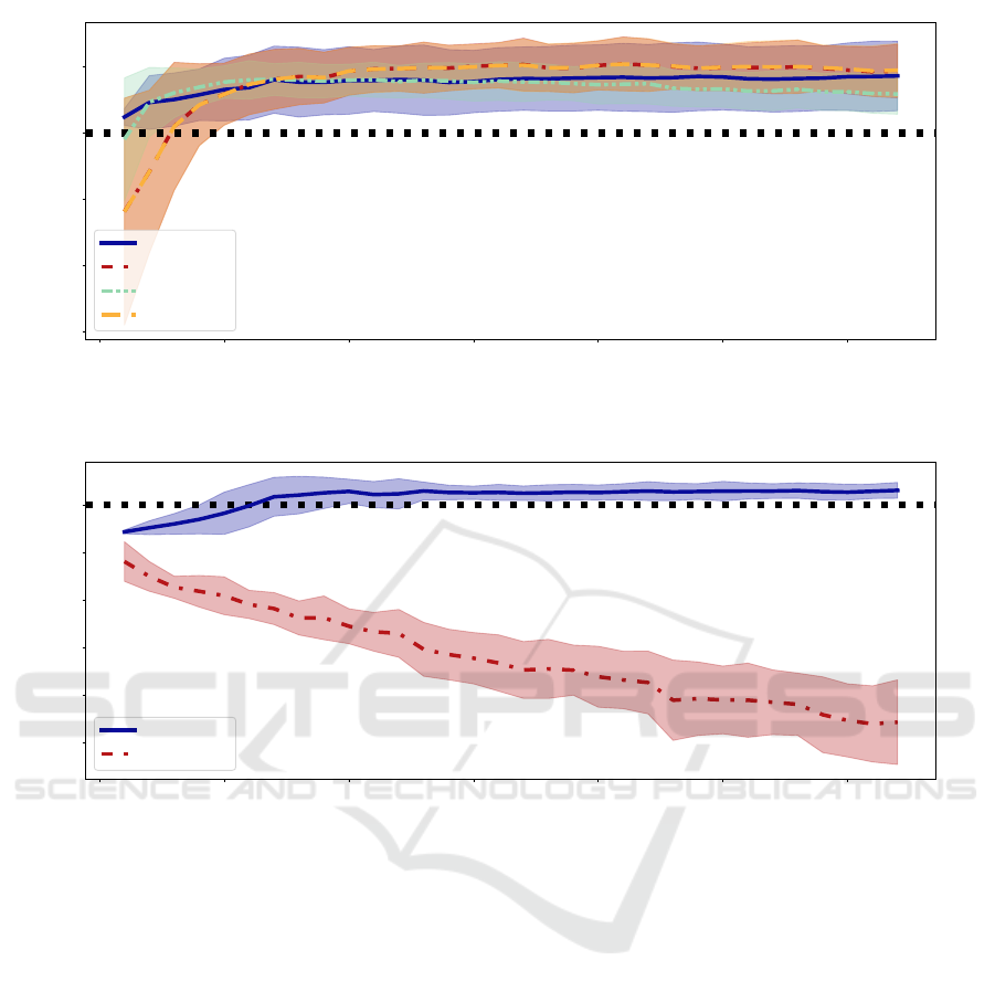
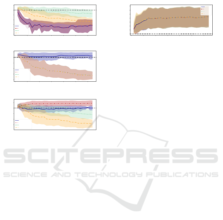
Results. Figure 2 visualizes the results of our de-

biasing experiments. We can see that for very small

numbers of tuning samples, our approach of param-

eter change penalization is beneﬁcial and leads to an

improvement in performance on the less biased test

distribution given as few as a single image. However,

for larger batch sizes, the baselines combined with our

stopping scheme reach similar and even slightly better

results on average.

To investigate the similar performance further, we

additionally visualize ||θ||

−||θ + θ

′

, i.e., the dif-

ference in the Euclidean norm of the model param-

eter vectors before and after the debiasing for our

approach and ﬁne-tuning. Figure 3 shows that even

though both methods achieve a similar increase in

performance for larger numbers of tuning samples,

they strive towards different optima. In fact, using

our approach, the Euclidean norm of the parameter

VISAPP 2024 - 19th International Conference on Computer Vision Theory and Applications

0 5 10 15 20 25 30

Number of Tuning Samples

−0.15

−0.10

−0.05

0.00

0.05

Balanced Accuracy Improvement

our method

ﬁne-tuning

side-tuning

MAS

Figure 2: The difference in accuracy after debiasing using our approach versus three baseline methods combined with our

stopping scheme on the melanoma classiﬁcation task.

0 5 10 15 20 25 30

Number of Tuning Samples

−0.0005

−0.0004

−0.0003

−0.0002

−0.0001

0.0000

Norm Diﬀerence

our method

ﬁne-tuning

Figure 3: Difference of the Euclidean norm of the model parameter vectors before and after the debiasing. Note that side-

tuning (Zhang et al., 2020) and MAS (Aljundi et al., 2018) lead to larger changes and overshadow the difference between our

approach and ﬁne-tuning. Hence, they are omitted here.

vector increases, which is possible because we penal-

ize change and do not perform classical weight decay.

We can also observe that our approach leads to, on av-

erage, smaller changes in the parameters θ due to our

regularization.

4.3 CelebA: Haircolor

Dataset. The second dataset we chose is the celebA

dataset (Liu et al., 2015) consisting of over 200K im-

ages picturing the faces of celebrities and annotated

with facial attributes. We use the implementation

from (Koh et al., 2021) and construct a simple bi-

nary classiﬁcation problem where the task is to decide

whether the hair color in an image is blond. However,

in our training distribution, all people with blond hair

are annotated as female in celebA, while we balance

not blond people between male and female celebri-

ties. Our biased models achieve, on average, a bal-

anced accuracy of 0.947 on this training distribution.

This performance drops to 0.779 on our test distribu-

tion, where no correlation between hair color and an-

notated sex exists. For debiasing, we only use images

of celebrities labeled as male with blond hair color.

Appendix 5 contains additional information and ex-

ample images of our data distributions.

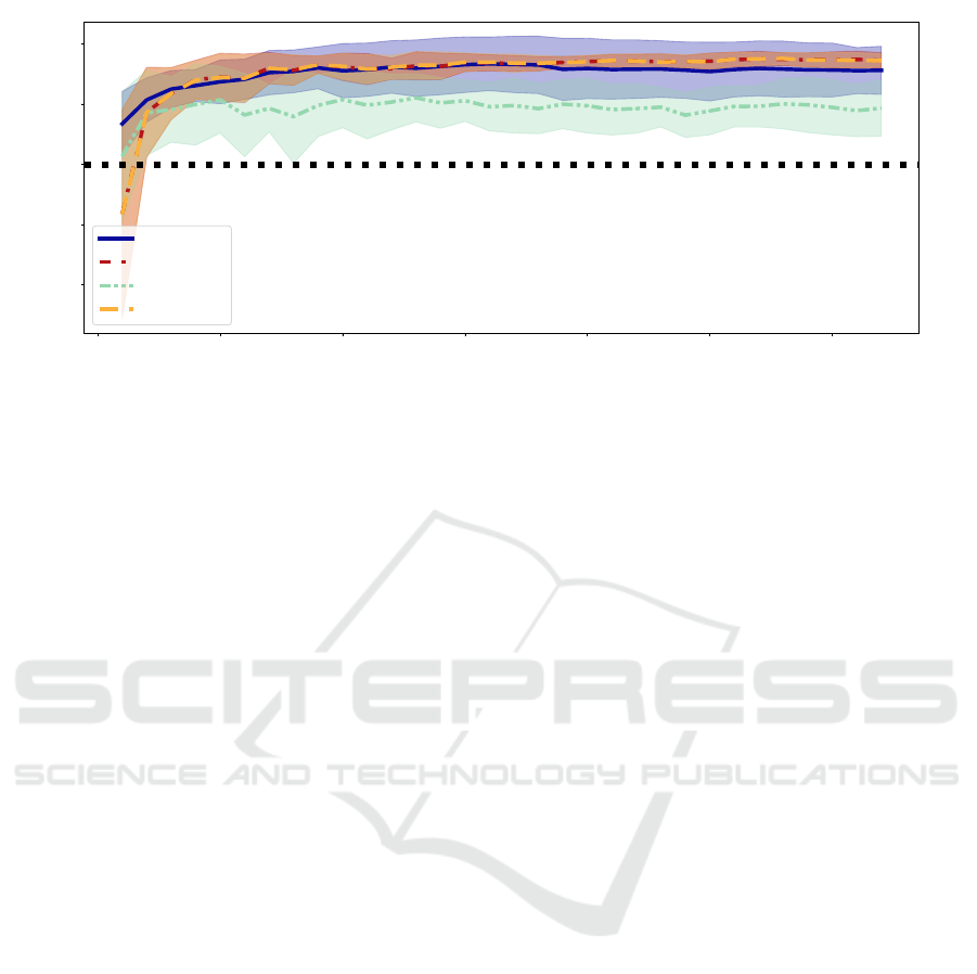
Results. The second task posed by the described

celebA (Liu et al., 2015) subset is conceptionally sim-

ilar to the ﬁrst problem we analyzed. Again we in-

vestigate a one-sided binary bias. Figure 4 visualizes

our results. Similar to our observations in Section 4.2,

here, our approach of change penalization leads to im-

provements as well, especially for smaller numbers of

tuning samples. Given larger batch sizes, the change

regularization implemented by our stopping criterion

Reducing Bias in Pre-Trained Models by Tuning While Penalizing Change

0 5 10 15 20 25 30

Number of Tuning Samples

−0.10

−0.05

0.00

0.05

0.10

Balanced Accuracy Improvement

our method

ﬁne-tuning

side-tuning

MAS

Figure 4: The difference in accuracy after debiasing using our approach versus three baseline methods combined with our

early stopping scheme on the celebA (Liu et al., 2015) classiﬁcation task.

combined with the baseline methods also results in

a performance increase. MAS and ﬁne-tuning per-

form near identical and lead, on average, to the high-

est increases for a number of 32 tuning samples. In

contrast, side-tuning is outperformed by the other ap-

proaches. Nevertheless, it still leads to an increase in

balanced accuracy.

4.4 Waterbirds: Bird Type

Dataset. Following the observation for the last two

datasets, i.e., that heavy change penalization can help

to improve simple one-sided binary biases, we now

investigate a two-sided bias. Toward this goal, we use

the waterbirds dataset (Sagawa et al., 2019) with the

implementation from (Koh et al., 2021). This dataset

is constructed by combining CUB200 (Wah et al.,

2011) birds together with Places (Zhou et al., 2017)

backgrounds. The task is to classify whether a dis-

played bird is a land or water-based species. However,

in the training distribution, there is a high correlation

between the label and a corresponding background

containing either land or water. Note that this means,

in contrast to the previous datasets we analyzed, that

there is still an overlap, i.e., some land birds are com-

bined with water images. Nevertheless, in the unbi-

ased test distribution, this correlation vanishes. The

balanced accuracies of our biased models, therefore,

decrease from 0.931 to 0.786 on average. See Ap-

pendix 5 for example images from this dataset. Note

that neither the training nor test data is class-wise bal-

anced. Hence, we compare the results for standard

accuracy and balanced accuracy. This comparison en-

ables us Finally, for debiasing, we use images from

the validation set, which follows the test distribution.

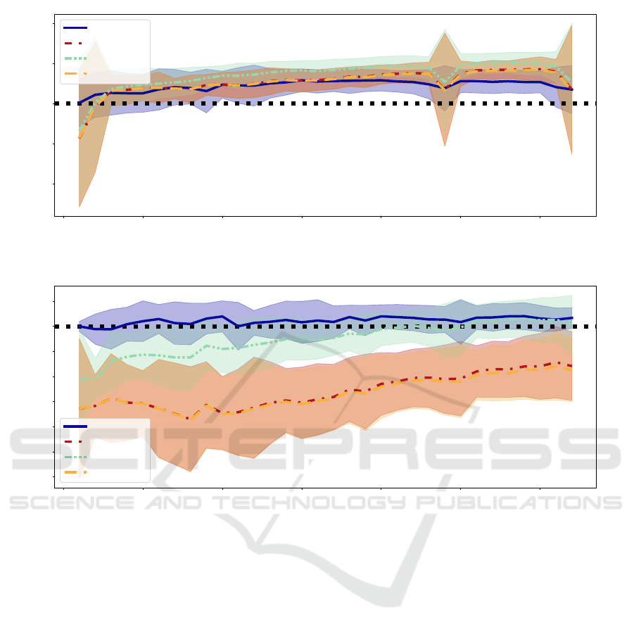
Results. For the more complicated two-sided bias

of the waterbirds dataset (Sagawa et al., 2019), we

analyze both the difference in accuracy and balanced

accuracy. Figure 5a shows that all methods lead to a

similar increase in standard accuracy. However, our

approach seems to perform slightly worse for larger

numbers of tuning samples. Yet, Figure 5b shows that

our approach does not degrade the balanced accuracy.

In contrast, while ﬁne-tuning and MAS lead to im-

provements in the unbalanced accuracy metric, they

drop the balanced accuracy by as much as 0.1. Both

methods perform worse for smaller amounts of tuning

samples. Side-tuning still drops the performance for

nearly all numbers of tuning samples but performs in

between our approach and the other two baselines.

4.5 Camelyon17: Cancer Tissue

Dataset. The last dataset of our analysis is the

camelyon17 dataset (Bandi et al., 2018). We select

this domain shift dataset given the similarity of our

deﬁnition of bias and domain shift in general. We use

the implementation from (Koh et al., 2021), where the

task is to classify whether images of tissue slides con-

tain cancerous tissue in the image center. However,

while the training data is collected from four different

hospital sites, the test data is captured in a disjunct in-

stitution leading to a clearly visible domain shift. See

Appendix 5 for examples. Given this domain shift,

the performances of our pre-trained models deterio-

rate from 0.996 on the train distribution down to 0.786

on the test distribution. For debiasing, we use held-

out images from the test split.

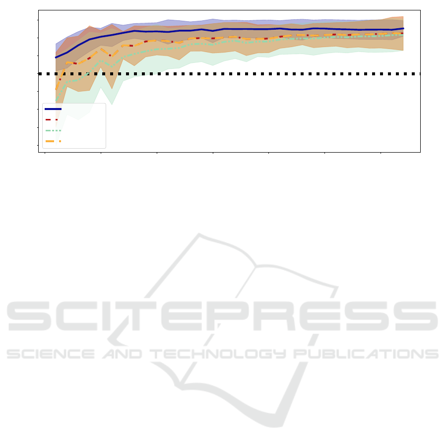
Results. Figure 6 visualizes the results for our last

set of experiments. Here our approach of change

VISAPP 2024 - 19th International Conference on Computer Vision Theory and Applications

0 5 10 15 20 25 30

Number of Tuning Samples

−0.10

−0.05

0.00

0.05

0.10

Accuracy Improvement

our method

ﬁne-tuning

side-tuning

MAS

(a) Difference in accuracy.

0 5 10 15 20 25 30

Number of Tuning Samples

−0.150

−0.125

−0.100

−0.075

−0.050

−0.025

0.000

0.025

Balanced Accuracy Improvement

our method

ﬁne-tuning

side-tuning

MAS

(b) Difference in balanced accuracy.

Figure 5: The differences in accuracy and balanced accuracy after debiasing using our approach versus three baseline methods

together with our early stopping scheme on the waterbirds dataset (Sagawa et al., 2019).

penalization performs best on average for all tested

numbers of tuning samples. Given only one tuning

sample, we can increase performance by around 0.05.

In contrast, the baselines decrease performance for

such little data. However, for a larger number of tun-

ing images, all methods increase the model perfor-

mance on the less biased test distribution. Again we

observe that MAS and ﬁne-tuning combined with our

stopping scheme lead to similar results.

5 CONCLUSIONS

In this work, we motivate the idea of debiasing pre-

trained image classiﬁcation models using heavy pe-

nalization of weight changes coupled with tuning

data contradicting learned biases. This approach fol-

lows the observation that models learn a combina-

tion of biases and meaningful features (Reimers et al.,

2021). To penalize change, we propose two methods

of change regularization: one based on an additional

loss function term and one early stopping scheme.

The latter of which can easily be added to existing

transfer learning approaches to lessen overﬁtting.

Our approach of adding a regularization term

leads to increased performance on less biased test

distributions of varied classiﬁcation tasks in our ex-

tensive empirical evaluation. This observation holds

true for as little as one image from the test sets.

Nevertheless, for larger numbers of tuning samples,

we conclude that it is often enough to utilize simple

ﬁne-tuning together with our early stopping scheme,

which leads to similar or better performance beneﬁts.

A future research direction is other penalization

metrics that could lead to further beneﬁts, e.g., the

spectral norm to force low-rank parameter changes.

Reducing Bias in Pre-Trained Models by Tuning While Penalizing Change

0 5 10 15 20 25 30

Number of Tuning Samples

−0.20

−0.15

−0.10

−0.05

0.00

0.05

0.10

0.15

Balanced Accuracy Improvement

our method

ﬁne-tuning

side-tuning

MAS

Figure 6: The difference in accuracy after debiasing using our approach versus three baseline methods together with our early

stopping scheme on the camelyon17 dataset (Bandi et al., 2018).

REFERENCES

International skin imaging collaboration, ISIC Archive.

https://www.isic-archive.com/.

Aljundi, R., Babiloni, F., Elhoseiny, M., Rohrbach, M.,

and Tuytelaars, T. (2018). Memory aware synapses:

Learning what (not) to forget. In Proceedings of

the European conference on computer vision (ECCV),

pages 139–154.

Bandi, P., Geessink, O., Manson, Q., Van Dijk, M., Balken-

hol, M., Hermsen, M., Bejnordi, B. E., Lee, B., Paeng,

K., Zhong, A., et al. (2018). From detection of indi-

vidual metastases to classiﬁcation of lymph node sta-

tus at the patient level: the camelyon17 challenge.

IEEE transactions on medical imaging, 38(2):550–

560.

Barone, A. V. M., Haddow, B., Germann, U., and Sen-

nrich, R. (2017). Regularization techniques for ﬁne-

tuning in neural machine translation. arXiv preprint

arXiv:1707.09920.

Brodersen, K. H., Ong, C. S., Stephan, K. E., and Buhmann,

J. M. (2010). The balanced accuracy and its posterior

distribution. In 2010 20th International Conference

on Pattern Recognition, pages 3121–3124.

Chelba, C. and Acero, A. (2006). Adaptation of maximum

entropy capitalizer: Little data can help a lot. Com-

puter Speech & Language, 20(4):382–399.

Ding, Y., Sheng, L., Liang, J., Zheng, A., and He, R. (2022).

Proxymix: Proxy-based mixup training with label

reﬁnery for source-free domain adaptation. arXiv

preprint arXiv:2205.14566.

Gira, M., Zhang, R., and Lee, K. (2022). Debiasing

pre-trained language models via efﬁcient ﬁne-tuning.

In Proceedings of the Second Workshop on Lan-

guage Technology for Equality, Diversity and Inclu-

sion, pages 59–69.

Goodfellow, I., Bengio, Y., and Courville, A. (2016). Deep

Learning. MIT Press. http://www.deeplearningbook.

org.

Gouk, H., Hospedales, T. M., and Pontil, M. (2021).

Distance-based regularisation of deep networks for

ﬁne-tuning.

He, K., Zhang, X., Ren, S., and Sun, J. (2015).

Deep Residual Learning for Image Recognition.

arXiv:1512.03385 [cs]. arXiv: 1512.03385.

Huang, J., Galal, G., Etemadi, M., and Vaidyanathan, M.

(2022). Evaluation and mitigation of racial bias in

clinical machine learning models: Scoping review.

JMIR Med. Inform., 10(5):e36388.

Ioffe, S. and Szegedy, C. (2015). Batch normalization: Ac-

celerating deep network training by reducing internal

covariate shift. In International conference on ma-

chine learning, pages 448–456. PMLR.

Koh, P. W., Sagawa, S., Marklund, H., Xie, S. M., Zhang,

M., Balsubramani, A., Hu, W., Yasunaga, M., Phillips,

R. L., Gao, I., et al. (2021). Wilds: A benchmark of in-

the-wild distribution shifts. In International Confer-

ence on Machine Learning, pages 5637–5664. PMLR.

Lee, J. and Lee, G. (2023). Feature alignment by uncer-

tainty and self-training for source-free unsupervised

domain adaptation. Neural Networks, 161:682–692.

Liang, J., Hu, D., and Feng, J. (2020). Do we really need

to access the source data? source hypothesis transfer

for unsupervised domain adaptation. In International

conference on machine learning, pages 6028–6039.

PMLR.

Liu, Z., Luo, P., Wang, X., and Tang, X. (2015). Deep learn-

ing face attributes in the wild. In Proceedings of In-

ternational Conference on Computer Vision (ICCV).

Mishra, N. K. and Celebi, M. E. (2016). An overview of

melanoma detection in dermoscopy images using im-

age processing and machine learning. arXiv preprint

arXiv:1601.07843.

Paszke, A., Gross, S., Massa, F., Lerer, A., Bradbury, J.,

Chanan, G., Killeen, T., Lin, Z., Gimelshein, N.,

Antiga, L., et al. (2019). Pytorch: An imperative style,

high-performance deep learning library. Advances in

neural information processing systems, 32.

VISAPP 2024 - 19th International Conference on Computer Vision Theory and Applications

Perkins, D. N., Salomon, G., et al. (1992). Transfer of learn-

ing. International encyclopedia of education, 2:6452–

6457.

Qu, S., Chen, G., Zhang, J., Li, Z., He, W., and Tao, D.

(2022). Bmd: A general class-balanced multicen-

tric dynamic prototype strategy for source-free do-

main adaptation. In European Conference on Com-

puter Vision, pages 165–182. Springer.

Reimers, C., Bodesheim, P., Runge, J., and Denzler, J.

(2021). Conditional adversarial debiasing: Towards

learning unbiased classiﬁers from biased data. In

DAGM German Conference on Pattern Recognition

(DAGM-GCPR), pages 48–62.

Rieger, L., Singh, C., Murdoch, W., and Yu, B. (2020).

Interpretations are useful: penalizing explanations to

align neural networks with prior knowledge. In In-

ternational conference on machine learning, pages

8116–8126. PMLR.

Roh, Y., Lee, K., Whang, S. E., and Suh, C. (2021). Fair-

batch: Batch selection for model fairness. In Interna-

tional Conference on Learning Representations.

Russakovsky, O., Deng, J., Su, H., Krause, J., Satheesh,

S., Ma, S., Huang, Z., Karpathy, A., Khosla, A.,

Bernstein, M., Berg, A. C., and Fei-Fei, L. (2015).

ImageNet Large Scale Visual Recognition Challenge.

International Journal of Computer Vision (IJCV),

115(3):211–252.

Sagawa, S., Koh, P. W., Hashimoto, T. B., and Liang, P.

(2019). Distributionally robust neural networks for

group shifts: On the importance of regularization for

worst-case generalization. In International Confer-

ence on Learning Representations.

Savani, Y., White, C., and Govindarajulu, N. S. (2020).

Intra-processing methods for debiasing neural net-

works. Advances in Neural Information Processing

Systems, 33:2798–2810.

Scope, A., Marchetti, M. A., Marghoob, A. A., Dusza,

S. W., Geller, A. C., Satagopan, J. M., Weinstock,

M. A., Berwick, M., and Halpern, A. C. (2016). The

study of nevi in children: Principles learned and im-

plications for melanoma diagnosis. J. Am. Acad. Der-

matol., 75(4):813–823.

Tartaglione, E., Barbano, C. A., and Grangetto, M. (2021).

End: Entangling and disentangling deep represen-

tations for bias correction. In Proceedings of the

IEEE/CVF conference on computer vision and pattern

recognition, pages 13508–13517.

Tian, J., Zhang, J., Li, W., and Xu, D. (2021). Vdm-da:

Virtual domain modeling for source data-free domain

adaptation. IEEE Transactions on Circuits and Sys-

tems for Video Technology, 32(6):3749–3760.

Wah, C., Branson, S., Welinder, P., Perona, P., and Be-

longie, S. (2011). The Caltech-UCSD Birds-200-2011

Dataset. Technical Report CNS-TR-2011-001, Cali-

fornia Institute of Technology.

Xuhong, L., Grandvalet, Y., and Davoine, F. (2018). Ex-

plicit inductive bias for transfer learning with convolu-

tional networks. In International Conference on Ma-

chine Learning, pages 2825–2834. PMLR.

Yao, Y., Rosasco, L., and Caponnetto, A. (2007). On early

stopping in gradient descent learning. Constructive

Approximation, 26:289–315.

Yu, Z., Li, J., Du, Z., Zhu, L., and Shen, H. T. (2023). A

comprehensive survey on source-free domain adapta-

tion. arXiv preprint arXiv:2302.11803.

Zhang, J. O., Sax, A., Zamir, A., Guibas, L., and Malik, J.

(2020). Side-tuning: a baseline for network adaptation

via additive side networks. In European Conference

on Computer Vision, pages 698–714. Springer.

Zhang, L., Rao, A., and Agrawala, M. (2023). Adding con-

ditional control to text-to-image diffusion models. In

Proceedings of the IEEE/CVF International Confer-

ence on Computer Vision, pages 3836–3847.

Zhou, B., Lapedriza, A., Khosla, A., Oliva, A., and Tor-

ralba, A. (2017). Places: A 10 million image database

for scene recognition. IEEE Transactions on Pattern

Analysis and Machine Intelligence.

Zhuang, F., Qi, Z., Duan, K., Xi, D., Zhu, Y., Zhu, H.,

Xiong, H., and He, Q. (2020). A comprehensive sur-

vey on transfer learning. Proceedings of the IEEE,

109(1):43–76.

APPENDIX

Colorful Patches Examples

Figure 7 displays examples of the original biased

training data and the melanomata with inpainted col-

orful patches we added to the test distribution. The

resulting less-biased test distribution contains benign

nevi and melanomata images with colorful patches.

(a) Original images of class nevus.

(b) Artiﬁcially inpainted melanoma images.

Figure 7: Some examples from biased training and less bi-

ased test distribution.

CelebA Examples

Figure 8 displays examples from the celebA dataset

(Liu et al., 2015) described in Section 4.3. We use

the implementation provided by (Koh et al., 2021) but

rebalance and resplit the dataset. Hence, the resulting

dataset is classwise balanced.

Reducing Bias in Pre-Trained Models by Tuning While Penalizing Change

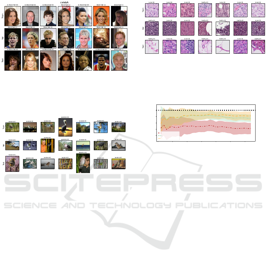
Figure 8: Examples contained in the celebA dataset (Liu

et al., 2015). All examples of class blond are female in the

train split (ﬁrst row). The row titled “val” contains tuning

examples, i.e., men with blond hair. The ﬁnal row contains

the test distribution, where men and women are uniformly

distributed in both classes.

Figure 9: Examples contained in the waterbirds dataset

(Sagawa et al., 2019). In the training distribution, birds

typically found in water-based environments correlate more

with water backgrounds, while land birds are often seen in

front of land-based backgrounds. For the validation, i.e.,

our tuning split and the test distribution, this correlation is

nearly zero.

Waterbirds Examples

Figure 9 contains examples of the waterbirds dataset

(Sagawa et al., 2019) described in Section 4.4. This

dataset is constructed with birds from the CUB-200

dataset (Wah et al., 2011) and backgrounds from the

Places dataset (Zhou et al., 2017). In the training-

split water and land-based birds correlate highly with

corresponding backgrounds. In contrast, the test dis-

tribution is more balanced, and the backgrounds and

birds are uncorrelated. We use the implementation

provided by (Koh et al., 2021).

Camelyon17 Examples

Figure 10 visualizes images contained in the came-

lyon17 dataset (Bandi et al., 2018). This dataset is

composed of similar images from different hospital

sites. These different capturing sites ensure a promi-

nent domain shift between training and test distribu-

tion. To ensure our tuning examples contain informa-

Figure 10: Examples from the camelyon17 dataset (Bandi

et al., 2018). The ﬁrst row contains images from the train-

ing distribution, which consists of images from four hos-

pital sites. The validation and test splits are composed of

images from disjunct hospitals, therefore, introducing a do-

main shift. We additionally split the test data to obtain our

tuning examples.

0 5 10 15 20 25 30

Number of Tuning Samples

−0.20

−0.15

−0.10

−0.05

0.00

Balanced Accuracy Improvement

ﬁne-tuning,  = 50

side-tuning,  = 50

MAS,  = 50

Figure 11: Baseline methods trained for 50 update steps

longer than our stopping criteria indicates. The black dotted

line indicates no change in balanced accuracy. All methods

lead to a decrease in performance.

tion about the test distribution, we split the original

test split provided by (Koh et al., 2021) to generate

our tuning batches. We provide more details about

our speciﬁc setup in Section 4.5.

Baseline Overﬁtting

In addition to our change penalization, we propose a

simple early-stopping scheme. We use this stopping

criterion to reduce overﬁtting on the tuning data for

our baseline methods. Here we now report what hap-

pens if we train the baseline approaches for ε = 50

update steps longer. For this comparison, we use the

dataset and setup described in Section 4.2.

Figure 11 shows the results for the amount of tun-

ing samples between 1 and 32. We see that the per-

formances of the pre-trained models on the test dis-

tribution deteriorate instead of increase. Hence, we

conclude that training for too long leads to overﬁtting

and reduces model performance signiﬁcantly. How-

ever, we can see that both side-tuning and especially

MAS, work better than classical ﬁne-tuning. MAS

already implicitly penalizes change to some parame-

ters, and side-tuning adds parameters and leaves the

original parameters untouched.

VISAPP 2024 - 19th International Conference on Computer Vision Theory and Applications

100

0 5 10 15 20 25 30

Number of Tuning Samples

−0.25

−0.20

−0.15

−0.10

−0.05

0.00

0.05

Balanced Accuracy Improvement

, λ = 10.0

, λ = 1.0

, λ = 0.1

, λ = 0.01

(a) ℓ

norm penalization.

0 5 10 15 20 25 30

Number of Tuning Samples

−0.20

−0.15

−0.10

−0.05

0.00

0.05

Balanced Accuracy Improvement

, λ = 1000.0

, λ = 10.0

, λ = 1.0

, λ = 0.1

, λ = 0.01

(b) ℓ

norm penalization.

0 5 10 15 20 25 30

Number of Tuning Samples

−0.15

−0.10

−0.05

0.00

0.05

Balanced Accuracy Improvement

+ `

, λ = 10.0

+ `

, λ = 1.0

+ `

, λ = 0.1

+ `

, λ = 0.01

+ ℓ

norm penalization.

Figure 12: Results for different parameter change norms.

For each norm, we visualize varying settings of the change

penalization parameter λ. For this evaluation, we set ε = 5

to ensure that the change penalization is larger than zero,

following the observations made in Section 3.1.

Hyperparameter Selection

Given computational constraints, we select the hy-

perparameters for our penalization approach on the

melanoma classiﬁcation problem described in Sec-

tion 4.2. Here, we describe the results of our small

ablation study and discuss the inﬂuence of the three

hyperparameters for our method: penalization norm,

penalization intensity λ, and stopping parameter ε.

First, we analyze the ﬁrst two hyperparameters ﬁrst.

For this, we set ε to ﬁve following the observation

made in Section 3.1. We test our approach for the ℓ

ℓ

, and 0.5 ·(ℓ

+ ℓ

) norms. Henceforth, we abbrevi-

ate the latter with ℓ

+ ℓ

Figure 12 shows varying settings of the parameter

λ for each of the three norms. First, we can see that

for the ℓ

norm and higher λ values, the tuning dete-

riorates completely. Remember that ℓ

regularization

leads to sparse solutions (Goodfellow et al., 2016),

i.e., the optimum for many parameters is zero. Hence,

only tuning a small number of parameters (for large

settings of λ) seems to be counterproductive. In con-

trast, it works better for smaller λ settings, especially

for smaller numbers of tuning samples, e.g., b = 1.

0 5 10 15 20 25 30

Number of Tuning Samples

0.00

0.01

0.02

0.03

0.04

0.05

0.06

0.07

Balanced Accuracy Improvement

 = 0

 = 5

 = 25

 = 100

Figure 13: Different settings for the stopping parameter ε.

Here we investigate our approach using the ℓ

+ ℓ

norm

together with λ = 1.0.

Nevertheless, for larger amounts of tuning samples,

performance still decreases. Using the ℓ

norm also

results in an increase in performance for smaller num-

bers of tuning samples given λ settings of 10 and

lower. In fact, all of these runs lead to very similar

parameters and, therefore, performance differences.

We argue that this behavior is overﬁtting similar to

the overﬁtting of long tuning observed in Appendix 5

indicated by the similar performance drop. Hence, we

additionally ran a set of experiments with λ = 1000.0

for ℓ

norm. For this setting, the models, on aver-

age, increase in performance. However, this setting

leads to convergence without correcting all tuning ex-

amples for large b, given the strong change penaliza-

tion. We, therefore, stop the tuning after 500 update

steps. Finally, Figure 12c visualizes the behavior of

our change penalization approach for the combined

ℓ

and ℓ

norms. Here we see that for very high pe-

nalization (λ = 10), the model performance for larger

batch sizes stays nearly constant compared to the pre-

trained model. Hence, penalization prevents change.

Values for λ lower than 1.0 deteriorate the model per-

formance, especially for larger b. For λ = 0.01, our

approach is closely related to standard ﬁne-tuning.

Here the setting ε = 5 could already lead to overﬁt-

ting on the tuning batches as observed in Appendix 5.

In contrast, λ = 1.0 leads to an improvement in the

performance metric for all analyzed numbers of tun-

ing samples. This effect is more pronounced for batch

sizes 7 and up.

To conclude: In this ﬁrst hyperparameter ablation,

we observe that in our setup for the melanoma classi-

ﬁcation task described in Section 4.2, the ℓ

+ℓ

norm

works best overall. Here we select λ = 1.0 as the pe-

nalization parameter. For this setup, we now investi-

gate different settings of the stopping criterion ε. Fig-

ure 13 visualizes results for ε values between 0 and

100. Our chosen set of hyperparameters is robust for

all settings of ε. All runs converge to indistinguish-

able performance increases. Hence, we select ε = 0

for our main experiments to increase comparability

with the extended baseline methods.

Reducing Bias in Pre-Trained Models by Tuning While Penalizing Change

101