
Biconic Approximation of a Toric Surface
Wei-Jun Chen
R&D Biometry, Ophthalmology, Carl Zeiss Meditec AG, G
¨
oschwitzer Straße 51–52, Jena, Germany
Keywords:
Biconic Model, Toric Lens, Sphere, Cylinder, Ellipsoid, Elliptic Cylinder, Astigmatism, Approximation.
Abstract:
In this work, a toric surface is explicitly approximated by a biconic model by decomposing the toric surface
into a biconic–identical component and other elliptical cylinder–related residual components. These residual
components determine the zone– and the azimuthal orientation–dependent approximation accuracy. In addi-
tion to the analytical underpinning, a direct fit of the biconic model to a data set sampled from a toric surface
is performed and consistent results are obtained.
1 INTRODUCTION
In geometrical optics as well as in ophthalmology
(cornea), an optical surface with the dominant opti-
cal aberration of astigmatism is usually called a toric
surface, which has two different refractive powers (re-
fractive curvatures) in two perpendicular meridians,
resulting in individual focal lengths.
There are three different but often intermingled
descriptions of a toric surface: 1, an optical surface
as a “cap” of a torus (Wiki-article, 2023); 2, an op-
tical surface as a composite “spherical + cylindrical”
surface (Barcala et al., 1995); 3, an optical surface de-
scribed by a biconic model with two different radii in
two perpendicular axes (e.g., the x– and y–axes).
In general, the first description of the “cap” of a
torus is often used to theoretically explain the geo-
metric properties of a toric surface, with the precise
mathematical definition being more visually under-
stood (Bartkowska, 1998) (Krasauskas, 2001), while
the second description is more of an industry– and
market–oriented description that provides an intuitive
understanding of the optical behavior of a toric lens.
The third description is a more engineering–oriented
description that is commonly used for optical design
and aberration compensation (Guo and Sun, 2017),
lens manufacturing (Chen et al., 2011), clinical tri-
als (P
´
erez-Escudero et al., 2010) (Janunts et al., 2015)
(Moore et al., 2019) (Giraudet et al., 2022) (Lan-
genbucher et al., 2023), scientific research in vari-
ous fields (Einighammer, 2008) (Gatinel et al., 2011)
(Pi
˜
nero et al., 2012) (Navarro et al., 2019) (Con-
sejo et al., 2021), etc. In addition, optical surfaces
with higher complexity, such as aspheres and higher–
order freeform surfaces, are often designed based on
a toric or biconic model plus additional conical con-
stants and individual Zernike components (Meister,
1998) (Roffman and Menezes, 1998) (Rosales et al.,
2009) (Scholz et al., 2009) (Gu et al., 2019) (Br
¨
omel,
2018) (Volatier et al., 2020).
Although the three descriptions above differ for-
mally, and have more or less their own flavor, they
attempt to provide consistent information about the
same optical aberration of astigmatism based on a
well–accepted assertion: For a true toric surface, a
biconic model with well–determined parameters is a
good approximation (Navarro, 2009). Nevertheless, it
is not so easy to find in the literature a direct answer
to the following question, namely how good such an
approximation is, for different specific applications.
An example of this can be found in Fig. 1, where
the comparable astigmatism of a toric and a biconic
model is illustrated by their refractive power maps
in the 12–mm zone
1
. However, the toric model also
has somewhat “asphericity” inside, while this is not
true for the biconic model, although these two models
have identical optical and geometric parameters.
With explicitly defined parameters of radius (r
a
)
and astigmatism (δ) for spherical and cylindrical sur-
faces, mathematical definitions of the toric surface
and the biconic model are rewritten in this paper.
Moreover, they are compared and decomposed into
their identical part and their distinct components,
where these distinct components are analogous to sev-
eral sums of polynomials of the astigmatism defined
elliptic cylinder, which explain well the intrinsic as-
1
The 12–mm and 6–mm zones are two typically relevant
zones in refractive laser surgery and cataract surgery.
Chen, W.
Biconic Approximation of a Toric Surface.
DOI: 10.5220/0012336800003651
Paper published under CC license (CC BY-NC-ND 4.0)
In Proceedings of the 12th International Conference on Photonics, Optics and Laser Technology (PHOTOPTICS 2024), pages 45-50
ISBN: 978-989-758-686-6; ISSN: 2184-4364
Proceedings Copyright © 2024 by SCITEPRESS – Science and Technology Publications, Lda.
45

(a) (b)
Figure 1: Refractive power maps of: (a) Toric model; (b)
Biconic model. Model parameters: r
a
= 6.88 mm, r
b
=
7.85 mm, cylinder axis = 31
◦
, refractive index = 1.3375,
map zone = 12 mm, map color unit = D (diopter).
phericity of a standard toric surface, and analytically
determine the quality of approximation of a biconic
model to a toric surface in a simple way.
The rest of this paper is organized as follows:
Sec. 2 rewrites the toric surface and the biconic model
with explicit optical parameters; Sec. 3 compares
these two models and decomposes them; the quality
of approximation of a biconic model to a toric sur-
face is first evaluated analytically in Sec. 4, and then
verified in Sec.4.1 by directly fitting a biconic model
to a discrete sample set taken from a predefined toric
surface; Sec. 5 discusses the evaluation results; finally
Sec. 6 concludes this paper with an expectation for fu-
ture work.
2 TORIC AND BICONIC MODELS
The standard toric surface as “cap” of a torus could be
defined by parametric equations
2
x = (c + a cosv)cosu
y = (c + a cosv)sinu
z = a sin v
(1)
describing a surface of revolution generated by the ro-
tation of a circle in 3D about the z–axis, where a de-
notes the radius of the circle, c the decentering of the
circle center from the z–axis, v the angular parameter
of the points on the circle, and u the angle of rotation.
If we move the coordinate origin to an optical ver-
tex on the surface from (x, y, z) →(x, y−(c+a).z) and
swap the axes y and z as (x, y, z ) → (x, −z, y), we get
x = (c + a cosv)cos u
z = (c + a) −(c + acosv) sin u
y = a sin v
(2)
which corresponds to
z = (c + a) −
r
c +
p
a
2
−y
2
2
−x
2
(3)
2
https://mathworld.wolfram.com/Torus.html
and in turn can be rewritten as
z = r
a
−
r
(r
a
−r
b
) +
q
r
2
b
−y
2
2
−x
2
(4)
where two radii are defined as r
a
= c + a and r
b
= a.
Extracting r
a
and r
b
from two squared root compo-
nents, we obtain
z = r
a
1 −
v
u
u
t
1 −
h
2
r
2
a
+ 2
r
2
b
r
a
δ
1 −
s
1 −
y
2
r
2
b
!
(5)
where h =
p
x
2
+ y
2
is the polar radius in the xy plane,
and δ =
1
r
a
−
1
r
b
is the astigmatism of the toric surface.
If we continue the Taylor expansion for two
squared root components in Eq. 5, we obtain:
z =
h
2
r
a
−δy
2
−2δ
y
2
∞
∑
k=1
p
k+1
y
2
r
2
b
k
!
×
∞
∑
m=0
p
m+1
h
2
r
2
a
+ ∆
r
y
2
+
δ
r
b
y
2
−
2δ
r
a
y
2
∞
∑
k=1
p
k+1
y
2
r
2
b
k
!
m
(6)
where p
m
=
1
2
,
1
8
,
1
16
,
5
128
,
7
256
, ... for m = 1, 2, 3, 4, 5, ...
are polynomial coefficients of f (x) = 1 −
√
1 −x, and
∆
r
= δ(δ −
2
r
a
) is an astigmatism dependent factor de-
rived from
1
r
2
b
=
1
r
2
a
+ ∆
r
.
On the other hand, the standard biconic model is
defined as
z =
x
2
r
a
+
y
2
r
b
1 +
r
1 −
x
2
r
2
a
(1 + k
a
) −
y
2
r
2
b
(1 + k
b
)
(7)
where k
a
and k
b
denote two conic constants and are
all zero when only astigmatism is considered. With
the above h, δ and ∆
r
, Eq. 7 is equivalent to
z =
h
2
r
a
−δy
2
h
2
r
2
a
+ ∆
r
y
2
1 −
s
1 −
h
2
r
2
a
+ ∆
r
y
2
!
(8)
which has also its polynomial version:
z =
h
2
r
a
−δy
2
!
×
∞
∑
m=0
p
m+1
h
2
r
2
a
+ ∆
r
y
2
!
m
. (9)
PHOTOPTICS 2024 - 12th International Conference on Photonics, Optics and Laser Technology
46
3 MODEL COMPARISON
Comparing Eq. 6 and Eq. 9, we see that the standard
toric surface as a “cap” of a torus contains a biconic
part. The Eq. 6 is then rewritten into
z =
H
δ
−E
!
×
∞
∑
m=0
p
m+1
H
∆
+
C
r
b
−
E
r
a
!
m
(10)
with
H
δ
=
h
2
r
a
−δy
2
(11)
H
∆
=
h
2
r
2
a
+ ∆
r
y
2
(12)
C = δy
2
(13)
E = 2C
∞
∑
k=1
p
k+1
y
2
r
2
b
k
(14)
where H
δ
and H
∆
contribute to the multiplier and the
multiplicand in the biconic model (Eq. 9), and C and
E denote a cylinder and an elliptical–cylinder, respec-
tively, inside the toric surface.
4 APPROXIMATION QUALITY
From the above Eqs.10–14, the approximation qual-
ity of a biconic model to a toric surface is determined
by the cylinder and elliptical–cylinder components in-
side a toric surface. If we subtract the biconic part
from a toric surface, we get the remainder as
z
rem
= z
toric
−z
biconic
=
H
δ
−E
∞
∑
m=1
m
∑
n=1
p
m+1
b
mn
×
H
m−n
∆
C
r
b
−
E
r
a
n
−
E
∞
∑
m=0
p
m+1
H
m
∆
(15)
where b
mn
denotes individual binomial coefficients.
The approximation error, i.e., the difference be-
tween a biconic model and its approximated toric sur-
face, can be calculated by Eq. 15. To facilitate the
analysis of zones and azimuthal orientation, the term
y
2
is replaced by h
2
sin
2
(ρ+ϕ) in all equations above,
where (h, ρ) denotes the polar coordinates of 2D po-
sitions in xy plane and ϕ the axis orientation of the
astigmatism. In the following analysis, the example
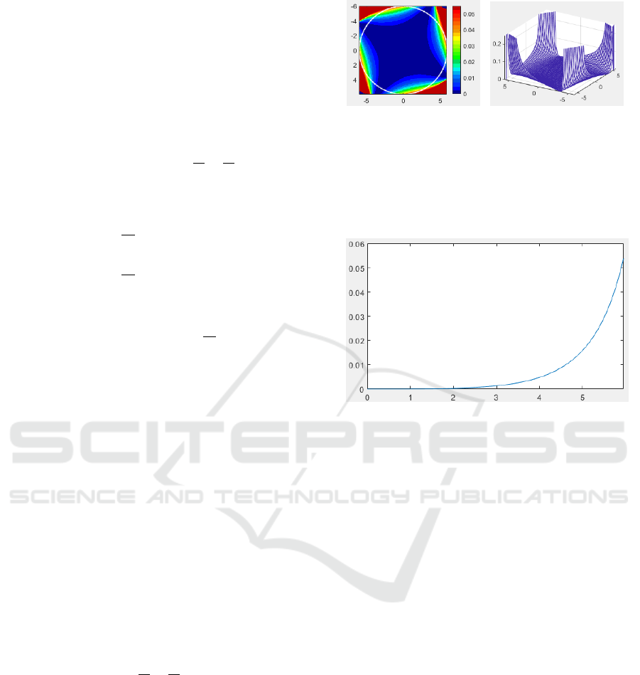
(a) (b)
Figure 2: Approximation error as the difference between
a true toric surface and its biconic approximation: (a)
Differential map z
rem
, where the color map illustrates the
value range from 0 to 0.05mm; (b) 3D mesh visualization
of the approximation error, where the value range in z axis
is from 0 to 0.25mm.
Figure 3: Zone dependence of the approximation error:
the curve of z
max
rem
(h) = max
ρ
z
rem
(h, ρ)|h ∈ [0 6mm], ρ ∈
[0
◦
360
◦
)
.
shown in Fig. 1 is evaluated using Eq. 15, and the ap-
proximation error is first illustrated in Fig. 2 for z
rem
over the whole 12 mm ×12 mm region.
The approximation error of a biconic model to a
true toric surface is zone dependent and also depends
on the azimuthal orientation. Using the model pa-
rameters given in Fig. 1, the zone dependence is il-
lustrated in Fig. 3. From this, it can be seen that
the maximum approximation erorr for the example
in Fig. 1 is ≈ 0.0012371 mm for a 6–mm zone (i.e.,
h ≤ 3 mm). The dependence on the azimuthal orienta-
tion is shown in Fig. 4, where 12 curves of z
rem
(h, ρ)
for individual h values are shown, the horizontal axis
being the azimuthal direction from 0
◦
to 360
◦
. It is
shown that the approximation error of the evaluated
example is lowest along the astigmatism axis ϕ and
its perpendicular axis (i.e., 31
◦
and 121
◦
for the ex-
ample in Fig. 1), while the maximum error is along
the azimuthal orientations of ϕ ±45
◦
.
The quality of approximation of a biconic model
to a true toric surface is also illustrated by the
differential refractive power map in Fig. 5, from
which we obtain the information that the maximum
approximation errors in the 6–mm zone and the 12–
mm zone are ≈ 0.36D and ≈ 3.22D, respectively.
Biconic Approximation of a Toric Surface
47
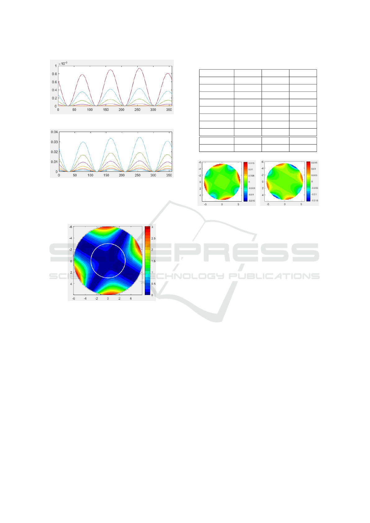
(a)
(b)
Figure 4: Azimuthal orientation dependence of the ap-
proximation error: the curve of z
rem
(h
k
, ρ) where h
k
=
k ×0.47 mm, and ρ ∈ [0
◦
360
◦
): (a); 6 curves for (h
k
|k =
0, 1, 2, ...5); (b) 6 curves for (h
k
|k = 6, 7, 8...11).
Figure 5: Evaluation of the approximation error by differen-
tiation of two refractive power maps, with two circles drawn
in the map to indicate the 6–mm zone and the 12–mm zone.
4.1 Biconic Model Fitting
In addition to the analytical evaluation of the qual-
ity of approximation of a biconical model to a given
true toric surface described above, this section de-
scribes an experimental evaluation by fitting a bi-
conic model to a discrete sample set, where the sam-
ple set X = (x
i
, y
i
, z
i
|i = 1, 2, ..., N) contains a total of
16384 points sampled within an 11–mm zone through
a regular 128 ×128 grid with a spatial resolution of
0.09375 mm on the xy plane, and the z–values were
calculated using the standard toric model (Eq. 4) with
model parameters of the example in Fig. 1. Sampling
in the 11–mm zone instead of the 12–mm zone serves
to avoid the surface edge effect.
A non–linear LeastSquares fitting was performed
Table 1: Biconic model fitting results.
Parameters Truth A–fit AC–fit
r
a
(mm) 6.88 6.8660 6.8669
r
b
(mm) 7.85 7.8260 7.8755
r
sph
(mm) 7.365 7.346 7.371
Sph (D) 45.8248 45.9434 45.7875
Cyl (D) 6.0616 6.0298 6.2944
ϕ (
◦
) 31
◦
31.0001 30.9997
k
a
0 0 -0.0001
k
b
0 0 0.0556
RMS (mm) 0 0.00359 0.00321
Max (mm) 0 0.016 0.015
(a) (b)
Figure 6: Fitting error maps: (a) The pure astigmatism fit;
(b) The astigmatism & conic fit.
based on the standard MATLAB optimization func-
tion lsqcurvefit and the standard biconic model
(Eq. 7). Two model fits were performed, one with
the model parameter for (r
a
, δ, ϕ) as a pure astigma-
tism fit (abbreviation: A–fit), and another with all the
biconical parameters (r
a
, δ, ϕ, k
a
, k
b
), namely an astig-
matism & conic fit (AC–fit).
The results of these two model fits are shown in
Table 1. From this, we can see that the estimation er-
rors of these two fits for the two perpendicular radii
are ≈ −0.014 mm for r
a
and ≈ ±0.025 mm for r
b
,
while the error for the astigmatism axis is quite small
(≈ 0.0002
◦
). Moreover, the AC–fit is slightly bet-
ter than the A–fit, in terms of the RMS criterion, but
all RMS are > 3 µm for the 11–mm zone. Mean-
while, the maximum error in the 11–mm zone is about
0.015 mm, which is consistent with the analytical
evaluation (Fig. 3).
The corresponding 2D error maps for these two
fits are shown in Fig. 6. In contrast to the analytical
evaluation (Fig. 2), these two model fits produce both
positive and negative errors because the least–squares
optimization is a compromise. For a better under-
standing of the fitting results, refractive power maps
of these two model fits are also shown in Fig. 7. From
these two maps, we know that the A-fit has the same
map structure as the theoretical result (Fig. 5), but
with a mean power shift of ≈ +0.12D, which is con-
sistent with the difference of the equivalence sphere
PHOTOPTICS 2024 - 12th International Conference on Photonics, Optics and Laser Technology
48
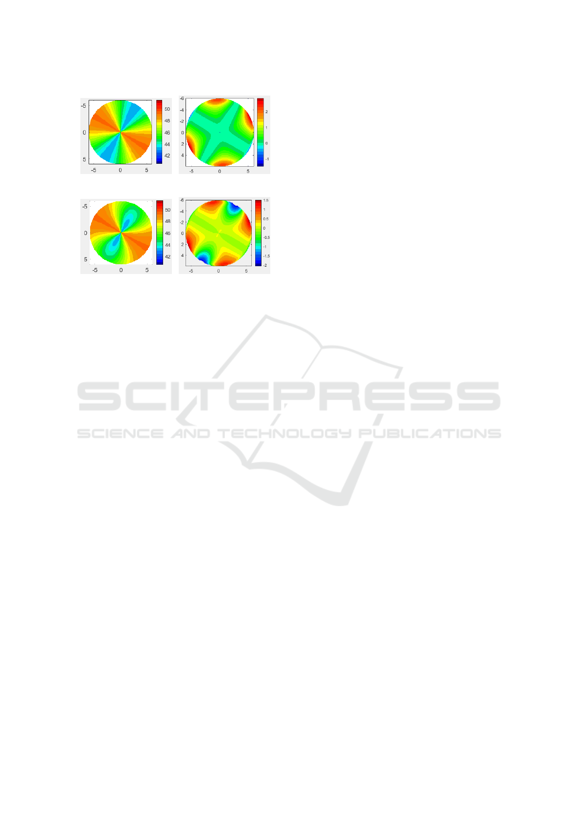
(a) (b)
(c) (d)
Figure 7: Model fitting results: (a), The refractive power
of the pure astigmatism fit; (b), The differential map as the
fitting residual of (a); (c), The refractive power of the astig-
matism & conic fit; (d), The differential map as the fitting
residual of (c).
(Sph in Table 1). On the other hand, the AC–fit pro-
duces a different power map structure due to the as-
phericity of two conical constants, which is different
from the asphericity resulting from the sums of the
polynomials of an elliptical cylinder on the toric sur-
face (Fig. 1(a)).
5 DISCUSSIONS
Based on the above theoretical and experimental un-
derpinning, approximating a biconic model to a toric
surface within a bounded zone, such as the 6–mm
zone for our example surface is good enough. If we go
beyond such a bounded zone, the approximation error
increases significantly, as shown in Fig. 3 and Fig. 4.
On the other hand, the approximation error is theo-
retically zero along the astigmatism axis and its per-
pendicular direction, while it periodically increases to
a maximum value at ≈ ±45
◦
from the astigmatism
axis. The approximation error is not random noise,
but structural deviation; the random noise is generally
expected to be suppressed by optimising the model
parameters, while the structural deviation is consid-
ered to be compensated by model selection and the
addition/removal of orthogonal components such as
Zernike components.
The interior of a toric surface contains an inher-
ent aspherical component, but it does not seem to
be readily described by conical constants in the bi-
conic model, as shown in Fig. 7(c) and Fig. 7(d).
Moreover, adjusting the conic constant in the biconic
model helps to reduce the RMS very slightly but non–
negligibly increases the approximation error of core
surface descriptors, such as the spherical radius and
the astigmatism, i.e. the K (keratometer) and the Cyl
(cylinder) values in the corneal clinic.
It should be noted that this paper investigates the
quality of approximation between two known mod-
els with available model parameters, which is only a
part of the full solution in many practical applications,
e.g., lens quality inspection, refractive modeling of
human corneal surfaces, etc. The focus of this work
is not to model the measured data by determining op-
timal parameters for a particular model, but rather
to provide a solid basis for the selection of torus or
biconical models with similar model parameters for
different geometries and refractive requirements.
6 CONCLUSIONS
It turns out that the quality of approximation of the
biconical model to a toric surface is good enough
within a bounded zone, while outside such a zone the
approximation error increases considerably. By rep-
resenting the standard toric model as a standard bi-
conic model plus remainder components, the approx-
imation error can be calculated analytically using the
torus parameters of the base sphere radius, astigma-
tism, and astigmatism axis. Meanwhile, these remain-
ing components are connected to an elliptical cylin-
der defined by the toric astigmatism as well as the
radius of the base sphere. This creates an intrinsic
aspheric structure within the toric surface that does
not directly correspond to the ellipsoid–like biconical
structure defined by two conical constants.
This work provides a solid foundation for further
research on the following three topics: First, from
the analysis of the remainder composition (Eq. 15),
the approximation acceptable zone should be explic-
itly determined by the torus parameters of astigma-
tism and base sphere; second, the choice of the model
for given measured data should take into account
different geometric structures under the same model
parameters, such as different aspherical structures in
the toric equation and the biconical equation; third,
it has been shown (Eqs. 6 and 9), but not further in-
vestigated, that both the toric model and the biconic
model are fully compatible with Zernike polynomi-
als. By combining individual Zernike components in
different ways, determining model parameters from
Zernike coefficients should be suitable for both of the
above aspheric structures.
Biconic Approximation of a Toric Surface
49

ACKNOWLEDGEMENTS
The author would like to thank his colleagues:
Christopher Weth, Tobias Buehen, Ziyao Tang, and
Carol Zhang, for their valuable technical discussions.
REFERENCES
Barcala, J., Vazquez, M. C., and Garcia, A. (1995). Optic
systems with spherical, cylindrical, and toric surfaces.
Applied Optics, 34(22):4900–4906.
Bartkowska, J. (1998). Toroidal surfaces in ophthalmic op-
tics. In Proceedings SPIE: Ophthalmic Measurements
and Optometry, volume 3579, pages 76–93.
Br
¨
omel, A. (2018). Dissertation: Development and
evaluation of freeform surface descriptions.
Friedrich–Schiller-Universit
¨
at Jena, Jena.
Chen, C.-C., Cheng, Y.-C., Hsu, W.-Y., Chou, H.-Y., Wang,
P. J., and Tsai, D. P. (2011). Slow tool servo diamond
turning of optical freeform surface for astigmatic con-
tact lens. In Optical Manufacturing and Testing IX,
volume 8126. Proc. of SPIE.
Consejo, A., Fathy, A., Lopes, B. T., Renato Ambr
´
osio, J.,
and Abass, A. (2021). Effect of corneal tilt on the
determination of asphericity. Sensors, 21(22):1–15.
Einighammer, J. (2008). Dissertation: The Individual Eye.
Eberhard-Karls-Universit
¨
at T
¨
ubingen, T
¨
ubingen.
Gatinel, D., Malet, J., Hoang-Xuan, T., and Azar, D. T.
(2011). Corneal elevation topography: Best fit sphere,
elevation distance, asphericity, toricity and clinical
implications. Cornea, 30(5):508–515.
Giraudet, C., Diaz, J., Tallec1, P. L., and Allain1, J.-
M. (2022). Multiscale mechanical model based on
patient-specific geometry: application to early kera-
toconus development. Journal of the Mechanical Be-
havior of Biomedical Materials, 129:1–13.
Gu, Y., McKenney, C. D., and Niculas, C. D. (2019).
Method for manufacturing toric contact lenese. US
Patent Application: US 2019/0193350 A1.
Guo, Y. and Sun, L. (2017). Biconic white multipass cell
design based on a skew ray–tracing model. Applied
Optics, 56(27):7586–7595.
Janunts, E., Kannengießer, M., and Langenbucher, A.
(2015). Parametric fitting of corneal height data to
a biconic surface. Zeitschrift f
¨
ur Medizinische Physik,
25(1):25–35.
Krasauskas, R. (2001). Shape of toric surfaces. In Proceed-
ings Spring Conference on Computer Graphics, pages
55–62.
Langenbucher, A., Szentm
´
ary, N., Cayless, A., Muen-
ninghoff, L., Wylegala, A., Wendelstein, J., and Hoff-
mann, P. (2023). Bootstrapping of corneal optical co-
herence tomography data to investigate conic fit ro-
bustness. Journal of Clinical Medicine, 12:1–16.
Meister, D. (1998). Principles of atoric lens design. Lens
Talk, 27(03):1–4.
Moore, J., Shu, X., Lopes, B. T., Wu, R., and Abass, A.
(2019). Limbus misrepresentation in parametric eye
models. PLoS ONE, 15(9):1–22.
Navarro, R. (2009). The optical design of the human eye: a
critical review. Journal of Optometry, 2(1):3–18.
Navarro, R., Rozema, J., Emamian, M. H., Hashemi, H.,
and Fotouhi, A. (2019). Average biometry of the
cornea in a large population of iranian school children.
Journal of the Optical Society of America A: Optics,
Image Science, and Vision, 36(4):B85–B92.
P
´
erez-Escudero, A., Dorronsoro, C., and Marcos, S. (2010).
Correlation between radius and asphericity in surfaces
fitted by conics. Journal of the Optical Society of
America A, 27(7):1541–1548.
Pi
˜
nero, D. P., Nieto, J. C., and Lopez-Miguel, A. (2012).
Characterization of corneal structure in keratoconus.
Journal of Cataract & Refractive Surgery, 38:2167–
2183.
Roffman, J. H. and Menezes, E. V. (1998). Aspheric toric
lens designs. US Patent: US 5796462.
Rosales, M. A., Ju
´
arez-Aubry, M., L
´
opez-Olazagasti, E.,
Ibarra, J., and Tepich
´
ın, E. (2009). Anterior corneal
profile with variable asphericity. Applied Optics,
48(35):6594–6599.
Scholz, K., Messner, A., Eppig, T., Bruenner, H., and Lan-
genbucher, A. (2009). Topography-based assessment
of anterior corneal curvature and asphericity as a func-
tion of age, sex, and refractive status. Journal of
Cataract & Refractive Surgery, 35:1046–1054.
Volatier, J.-B., Duveau, L., and Druart, G. (2020). An ex-
ploration of the freeform two–mirror off–axis solution
space. Journal of Physics: Photonics, 2:1–9.
Wiki-article (2023). Toric lens.
https://en.wikipedia.org/wiki/Toric lens.
PHOTOPTICS 2024 - 12th International Conference on Photonics, Optics and Laser Technology
50
