Fault Tree Reliability Analysis via Squarefree Polynomials

Milan Lopuha

a-Zwakenberg

University of Twente, Enschede, The Netherlands

Keywords:

Fault Trees, Reliability Analysis, Polynomial Algebra.

Abstract:

Fault tree (FT) analysis is a prominent risk assessment method in industrial systems. Unreliability is one of the

key safety metrics in quantitative FT analysis. Existing algorithms for unreliability analysis are based on binary

decision diagrams, for which it is hard to give time complexity guarantees beyond a worst-case exponential

bound. In this paper, we present a novel method to calculate FT unreliability based on algebras of squarefree

polynomials and prove its validity. We furthermore prove that time complexity is low when the number of

multiparent nodes is limited. Experiments show that our method is competitive with the state-of-the-art and

outperforms it for FTs with few multiparent nodes.

1 INTRODUCTION

Fault trees. Fault trees (FTs) form a prominent risk

assessment method to categorize safety risks on in-

dustrial systems. A FT is a hierarchical graphical

model that shows how failures may propagate and

lead to system failure. Because of its ﬂexibility and

rigor, FT analysis is incorporated in many risk assess-

ment methods employed in industry, including Fault-

Tree+ (IsoTree, 2023) and TopEvent FTA (Reliotech,

2023).

A FT is a directed acyclic graph (not necessarily a

tree) whose root represents system failure. The leaves

are called basic events (BEs) and represent atomic

failure events. Intermediate nodes are AND/OR-

gates, whose activation depends on that of their chil-

dren; the system as a whole fails when the root is ac-

tivated. An example is given in Fig. 1.

Quantitative analysis. Besides a qualitative analy-

sis of what sets of events cause overall system fail-

ure, FTs also play an important role in quantitative

risk analysis, which seeks to express the safety of the

system in terms of safety metrics, such as the total

expected downtime, availability, etc. An important

safety metric is (un)reliability, which, given the fail-

ure probability of each BE, calculates the probability

of system failure. As the size of FTs can grow into the

hundreds of nodes (Ruijters et al., 2019), calculating

the unreliability efﬁciently is crucial for giving safety

and availability guarantees.

There exist two main approaches to calculating

unreliability (Ruijters and Stoelinga, 2015). The ﬁrst

Left engine fails Right engine fails

Right rotor fails Left rotor failsNo fuel

AND

Aircraft fails

Figure 1: A fault tree for a small aircraft. The aircraft fails

if both its engines fail; each engine fails if either its rotor

fails or it has no fuel (the plane has a single fuel tank).

approach works bottom-up, recursively calculating

the failure probability of each gate. This algorithm is

fast (linear time complexity), but only works as long

as the FT is actually a tree. However, nodes with mul-

tiple parents (DAG-like FTs) are necessary to model

more intricate systems. For such FTs, as we show in

this paper, calculating unreliability is NP-hard. The

main approach for such FTs is based on translating

the FT into a binary decision diagram (BDD) and per-

forming a bottom-up analysis on the BDD. This BDD

is of worst-case exponential size, though heuristics

exist. The BDD corresponding to an FT depends on

a linear ordering of the BEs, with different orderings

yielding BDDs of wildly varying size; although any

single one of them can be used to calculate unrelia-

bility, ﬁnding the optimal BE ordering is an NP-hard

problem in itself. As a result, it is hard to give guar-

antees on the runtime of this unreliability calculation

algorithm in terms of properties of the FT.

Lopuhaä-Zwakenberg, M.

Fault Tree Reliability Analysis via Squarefree Polynomials.

DOI: 10.5220/0012334000003645

Paper published under CC license (CC BY-NC-ND 4.0)

In Proceedings of the 12th International Conference on Model-Based Software and Systems Engineering (MODELSWARD 2024), pages 39-49

ISBN: 978-989-758-682-8; ISSN: 2184-4348

Contributions. In this paper, we present a radical

new way for calculating unreliability for general FTs.

The bottom-up algorithm does not work for DAG-like

FTs, since it does not recognize multiple copies of the

same node in the calculation, leading to double count-

ing. In our approach we amend this by keeping track

of nodes with multiple parents, as these may occur

twice in the same calculation. Then, instead of propa-

gating failure probabilities as real numbers, we prop-

agate squarefree polynomials whose variables repre-

sent the failure probabilities of nodes with multiple

parents; keeping these formal variables allows us to

detect and account for double counting. Furthermore,

to keep complexity down we replace formal variables

with real numbers whenever we are able. At the root

all formal variables have been substituted away, yield-

ing the unreliability as a real number.

This approach has as advantage over BDD-based

algorithms that we are able to give upper bounds to

computational complexity. Most of the complexity

comes from the fact that we do arithmetic with poly-

nomials rather than real numbers. However, if the

number of multiparent nodes is limited, these poly-

nomials have limited degree, and computation is still

fast. We prove this formally, by showing that the time

complexity is linear when the number of multipar-

ent nodes is bounded, and in experiments, in which

we compare our method to Storm-dft (Basg

oze et al.,

2022b), a state-of-the-art tool for FT analysis using a

BDD-based approach: here our method is competitive

in general and is considerably faster for FTs with few

multiparent nodes.

Summarized our contributions are the following:

1. A new algorithm for fault tree reliability analysis

based on squarefree polynomial algebras;

2. A proof of the algorithm’s validity and bounds on

its time complexity;

3. Experiments comparing our algorithm to the

state-of-the-art.

An artefact of the experiments is available at (Lop-

uha

a-Zwakenberg, 2023a). Furthermore, a version of

this paper including proofs of the mathematical state-

ments is available at (Lopuha

a-Zwakenberg, 2023b).

2 RELATED WORK

There exists a considerable amount of work on FT re-

liability analysis. FTs were ﬁrst introduced in (Wat-

son, 1961). A bottom-up algorithm to calculate their

reliability is presented in (Ruijters and Stoelinga,

2015), which is a formalization of mathematical prin-

ciples that have been used since the beginning of FT

analysis. This algorithm works only for FTs that are

actually trees, i.e., do not contain nodes with multiple

parents. In (Rauzy, 1993), a BDD-based method for

calculating reliability was introduced that also works

for DAG-shaped FTs. This method is still the state

of the art, although some improvements have been

made, notably by tweaking variable ordering to ob-

tain smaller BDDs (Bouissou et al., 1997) and divid-

ing the FT into so-called modules that can be handled

separately (Rauzy and Dutuit, 1997).

FTs are also used to model the system’s reliabil-

ity over time. The failure time of each BE is mod-

eled as a random variable (typically exponentially dis-

tributed), and additional gate types are introduced to

model more elaborate timing behavior. Reliability

analysis of these dynamic FTs is done via stochastic

model checking (Basg

oze et al., 2022b).

3 FAULT TREES

In this section, we give the formal deﬁnition of fault

trees (FTs) and their reliability used in this paper. For

us FTs are static (only AND/OR gates), and each ba-

sic event v is assigned a failure probability p(v). Thus

we deﬁne:

Deﬁnition 3.1. A fault tree (FT) is a tuple T =

(V, E,γ,p) where:

• (V, E) is a rooted directed acyclic graph;

• γ is a function γ: V → {OR, AND, BE} such that

γ(v) = BE if and only if v is a leaf;

• p is a function p : BE

→ [0,1], where BE

{v ∈ V | γ(v) = BE}.

Note that a FT is not necessarily a tree as gates

may share children. The root of T is denoted R

. For

a node v, we let ch(v) be the set of children of v.

The structure function determines, given a gate

and a safety event, whether the event succesfully

propagates to the gate. Here we model a safety event

as the set of BEs happening, which can be encoded as

a binary vector

f ∈ B

, where f

= 1 denotes that

the BE v occurs in the event. The structure function is

then deﬁned as follows.

Deﬁnition 3.2. Let T = (V,E,γ,p) be a FT.

1. A safety event is an element of B

2. The structure function of T is the function

: V × B

→ B deﬁned recursively by

(v,

f ) =











, if γ(v) = BE,

w∈ch(v)

(w,

f ), if γ(v) = OR,

w∈ch(v)

(w,

f ), if γ(v) = AND.

MODELSWARD 2024 - 12th International Conference on Model-Based Software and Systems Engineering

3. A safety event

f such that S

f ) = 1 is called

a cut set; the set of all cut sets is denoted CS

Quantitative analysis of a FT is typically done via

its unreliability, i.e., the probability of a cut set occur-

ring, where each BE v has probability p(v) of happen-

ing. The BE failure probabilities are considered to be

independent. The reasoning behind this is that when

they are not independent, this is due to some common

cause; this common cause should then be explicitely

modeled in the FT framework, by replacing the two

non-independent BEs with sub-FTs that share com-

mon nodes (Pandey, 2005).

Deﬁnition 3.3. Let T = (V,E,γ,p) be a FT. Let

F ∈

be the random variable deﬁned by P(F

= 1) =

p(v) for all v ∈ BE

, and all these events are indepen-

dent. Then the unreliability of T is deﬁned as

U(T) = P(

F ∈ CS

)

∑

f ∈CS

∏

v: f

p(v)

∏

v: f

(1 − p(v)).

Example 3.4. Consider the FT T from Fig. 1. Ab-

breviating BE names, assume p(rrf) = p(lrf) = 0.4

and p(nf) = 0.3. Furthermore, write

f ∈ B

rrf

lrf

. Then CS

= {010,011,101,110,111}, so

U(T ) = 0.6 · 0.3 · 0.6

+ 0.6 · 0.3 · 0.4

+ 0.4 · 0.7 · 0.4

+ 0.4 · 0.3 · 0.6

+ 0.4 · 0.3 · 0.4 = 0.412.

The unreliability U(T ) represents the probability

of failure of the system modeled by the fault tree and

is crucuial to providing safety and availability guar-

antees. The expression in Deﬁnition 3.3 becomes too

large to handle for large FTs very quickly; thus it is

important to ﬁnd efﬁcient solutions to the following

problem.

Problem 3.5. Given a FT T , calculate U(T ).

Unfortunately, we show that this problem is NP-

hard. The reason for this is that with appropriately

chosen probabilities, one can ﬁnd from U(T ) a mini-

mal element of CS

, and ﬁnding such a so-called min-

imal cut set is known to be NP-hard (Rauzy, 1993).

Theorem 3.6. Problem 3.5 is NP-hard.

3.1 Existing U(T ) Algorithms

There are two prominent algorithms for calculating

U(T ). The ﬁrst one calculates, for each node v, the

probability g

= P(S

(v,

F) = 1) bottom-up (Ruijters

and Stoelinga, 2015). For BEs one has g

= p(v). For

a b

d e

0.5 0.5 0.5

0.5

Figure 2: An example FT with failure probabilities.

an AND-gate, one has g

∏

w∈ch(v)

as long as the

events S

(w,

F) = 1 are independent as w ranges over

all children of v. This happens when no two children

of v have any shared descendants. For OR-gates one

likewise has g

= 1 −

∏

w∈ch(v)

. This gives rise to

a linear-time algorithm that calculates g

bottom-up.

Unfortunately, this algorithm only works for FTs that

have a tree structure: as soon as a node has multiple

parents, the independence assumption will be violated

at some point in the calculation.

The second algorithm (Rauzy, 1993) works for

general FTs, and works by translating the Boolean

function S

,−) into a binary decision diagram,

which is a directed acyclic graph, in which the eval-

uation of the function at a boolean vector is repre-

sented by a path through the graph. After the BDD

is found, U(T ) can be calculated using a bottom-up

algorithm on the BDD, whose time complexity is lin-

ear in the size of the BDD. Unfortunately, the size

of the BDD is worst-case exponential, although this

worst case is seldomly attained in practice (Rauzy and

Dutuit, 1997; Bobbio et al., 2013). To construct the

BDD, one ﬁrst has to linearly order the variables; ﬁnd-

ing the order that minimizes BDD size is an NP-hard

problem, although heuristics exist (Valiant, 1979; L

et al., 2014).

4 AN EXAMPLE OF OUR

METHOD

Before we dive into the details of our method, we

go through an example to showcase how the method

works and to motivate the technical sections.

Consider the FT of Fig. 2. In a bottom-up method,

we calculate the failure probability g

of each node v:

thus for the BEs we have g

= g

= 0.5.

For d, the bottom-up method dictates that we should

calculate g

= g

+ g

− g

. However, this will

Fault Tree Reliability Analysis via Squarefree Polynomials

cause problems at f , since d and e share b as child,

and so their failure probabilities will not be indepen-

dent. Thus, at d, we modify g

to ‘remember’ its de-

pendence on b. We do so by introducing a formal

variable L

representing b’s failure probability, yield-

ing g

= g

+ L

− g

= 0.5 + 0.5L

. We also get

= 0.5 + 0.5L

. Note that we only introduce a for-

mal variable for b, and not for a and c, as the latter

only have one parent node and thus have no chance of

appearing twice in the same calculation.

At f , we calculate g

= g

= 0.25 + 0.5L

0.25L

. Here we introduce the rule L

= L

, so that

= 0.25 + 0.75L

. The idea behind this is that

we use multiplication to determine the possibility of

two events occurring simultaneously. Since L

rep-

resents P(S

(b,

F) = 1), the term L

actually repre-

sents P(S

(b,

F) = 1 ∧ S

(b,

F) = 1). This is equal

to P(S

(b,

F) = 1), so L

= L

At this point, the graph structure tells us that b

cannot appear twice in the same calculation any more.

Thus we can safely substitute g

= 0.5 for L

in g

0.25 + 0.75L

, yielding g

= 0.625. Finally, we get

= g

= 0.3125.

In the following sections, we introduce two math-

ematical tools needed to apply this method in greater

generality. In Section 5 we review the graph-theoretic

notion of dominators, which will tell us for which

nodes we need to introduce formal variables and at

what point they can be substituted away. In Section

6 we formalize the polynomial algebra in which our

arithmetic takes place.

5 PRELIMINARIES I:

DOMINATORS

In this section we review the concept of dominators

and apply them to FTs. We need this to determine at

what point in the bottom-up calculation, outlined in

the previous section, we can replace a formal variable

with the expression g

. Informally, a dominator of

v is present on all paths from the root to v.

Deﬁnition 5.1. (Prosser, 1959) Let T = (V,E, γ, p) be

a FT.

1. Deﬁne a partial order  on V by x  y iff there is

a path y → x in T .

2. Given two nodes v,w ∈ V , we say that w dominates

v if v ≺ w and every path R

→ v in T contains w.

The set of dominators of a node is nonempty and

has a minimum:

Lemma 5.2. (Lengauer and Tarjan, 1979) If v 6= R

then there is a unique w dominating v such that each

dominating v satisﬁes w  w

; this w is called the

immediate dominator of v, denoted w = id(v).

Example 5.3. In Fig. 2, the dominators of a are d, f ,

and h, and id(a) = d. The dominators of b are f and

h, and id(b) = f . Note that d is not a dominator of b,

since the path h → f → e → b does not pass through

The immediate dominator is interesting to us

since, as we will see later, at id(v) we can replace L

by g

. The following result relates the relative posi-

tion of v and w to that of their immediate dominators.

Lemma 5.4. If v ≺ w, then either id(v)  w or

id(w)  id(v).

To use these deﬁnitions in an algorithmic context,

we will make use of the following result:

Theorem 5.5. (Lengauer and Tarjan, 1979) Given T ,

there exists an algorithm of time complexity O(|E|)

that ﬁnds id(v) for each v ∈ V .

6 PRELIMINARIES II:

SQUAREFREE POLYNOMIAL

ALGEBRAS

In this second preliminary section, we formally de-

ﬁne the algebras in which our calculations take place.

These are similar to multivariate polynomial algebras,

except in every monomial every variable can have de-

gree at most 1.

Deﬁnition 6.1. Let X be a ﬁnite set. We deﬁne the

squarefree real polynomial algebra over X to be the

algebra A(X) consisting of formal sums

α =

∑

Y ⊆X

∏

x∈Y

where the L

are formal variables and α

∈ R. Ad-

dition and multiplication are as normal polynomials,

except that they are subject to the law L

= L

for all

x ∈ X; that is,

(α + β)

= α

+ β

(α · β)

∑

⊆X :

∪Y

Example 6.2. Let X = {x, y}. Let α = 2 + L

+ L

and β = L

+ 3L

. Coefﬁcientwise, α is described











2, if X = ∅,

1, if X = {x} or X = {y},

0, if X = {x, y}.

Furthermore, α + β = 2 + 2L

+ L

+ 3L

, and

α · β = α · L

+ α · (3L

)

MODELSWARD 2024 - 12th International Conference on Model-Based Software and Systems Engineering

= (2L

+ L

) + (6L

+ 3L

)

= 3L

+ L

+ 9L

+ 3L

Note that if X ⊆ X

, an α ∈ A (X) can also be con-

sidered an element of A(X

), by taking α

= 0 when-

ever Y 6⊆ X. For two sets X and Y this also allows us

to add and multiply α ∈ A(X ) and β ∈ A (Y ), by con-

sidering both to be elements of A (X ∪Y ). In the rest

of this paper we will do this without comment.

Besides multiplication and addition, another im-

portant operation that we need is the substitution of a

formal variable by a polynomial. This works the same

as with regular polynomials.

Deﬁnition 6.3. Let X,Y be ﬁnite sets and x ∈ X \Y .

Let α ∈ A (X) and β ∈ A(Y ). Then the substitution

α[L

7→ β] is the element of A (X \ {x} ∪Y ) obtained

by replacing all instances of L

by β; more formally,

α[L

7→ β] is expressed as

β ·







∑

Z⊆X :

x∈Z

∏

∈Z\{x}







∑

Z⊆X :

x /∈Z

∏

∈Z

In terms of coefﬁcients this is expressed as

α[L

7→ β]

= α

∑

x∈Z

⊆X,

⊆Y :

\{x}∪Z

where α

= 0 if Z 6⊆ X.

Note that in this deﬁnition the multiplication and

addition are of elements of A(X \{x} ∪Y ).

Example 6.4. Continuing Example 6.2, the substitu-

tion β[L

7→ α] is equal to

β[L

7→ α] = L

+ 3L

· (2 + L

+ L

)

= 10L

+ 3L

In what follows, we will need three results on cal-

culation in A(X). The ﬁrst result considerably sim-

pliﬁes the substitution operation.

Lemma 6.5. Let x,α,β be as in Deﬁnition 6.3. Then

α[L

7→ β] = α[L

7→ 1] · β + α[L

7→ 0] · (1 − β).

The second result shows how substitution behaves

with respect to addition and multiplication.

Lemma 6.6. Let α

,α

∈ A(X), β ∈ A (Y ), and x ∈

X \Y . Then:

1. (α

+ α

)[L

7→ β] = α

7→ β] + α

7→ β].

2. If β

= β, then furthermore (α

)[L

7→ β] =

7→ β] · α

7→ β].

The third result states that two substitution oper-

ations can be interchanged, as long as one does not

substitute a variable present in the other:

Lemma 6.7. Let α ∈ A(X), β

∈ A (Y

), β

∈ A (Y

∈ X \ (Y

∪ Y

). If x

/∈ Y

and x

/∈ Y

, then

α[L

7→ β

][L

7→ β

] = α[L

7→ β

][L

7→ β

When this lemma applies and the order of substi-

tutions does not matter, we will write expressions like

α[L

7→ β

], or even α[∀i ≤ n : L

7→ β

Note that as an R-algebra, one may identify A(X )

with K/I, where K = R[L

: x ∈ X] is a free polyno-

mial algebra and I is the ideal generated by the set

− L

| x ∈ X}. However, the substitution opera-

tion does not correspond to a ‘natural’ operation on

on K/I.

6.1 Real-Valued Boolean Functions

We will use the elements of A (X) is to represent func-

tions B

→ R. The following result states that this

can be done in a unique way. Since both elements of

A(X) and functions B

→ R can be represented by

|X|

real numbers, this should come as no surprise.

Theorem 6.8. Let X be a ﬁnite set, and let g: B

→

R be any function. Then there exists a unique hgi ∈

A(X) such that g(c) = hgi[∀x ∈ X : L

7→ c

] for all

~c ∈ B

Example 6.9. Let X = {x,y}, with ~c ∈ B

repre-

sented as c

. Consider the function g: B

→ R

given by

g(00) = 3, g(01) = −2,

g(10) = 7, g(11) = 4.

Suppose hgi = k

+ k

. Then, for

instance,

g(10) = hgi[L

7→ 1,L

7→ 0] = k

+ k

In a similar way we can express all g(~c) as sums of k

Thus, to ﬁnd the k

, we have to solve







1 0 0 0

1 1 0 0

1 0 1 0

1 1 1 1

























−2







Since this matrix is lower triangular with nonzero di-

agonal entries, it is invertible, so the k

exist and are

unique. In fact, we ﬁnd hgi = 3 + 4L

− 5L

+ 2L

7 THE ALGORITHM

Using the notation of the previous two sections, we

can now state our algorithm for calculating unrelia-

bility. It is presented in Algorithm 1. The algorithm

works bottom-up, assigning to each node v a formal

Fault Tree Reliability Analysis via Squarefree Polynomials

input : A FT T = (V,E,γ,p)

output: U (T )

1 ToDo ← V ;

2 while ToDo 6= ∅ do

3 Pick v ∈ ToDo minimal w.r.t. ;

4 ToDo ← ToDo \ {v};

5 if γ(v) = BE then

6 g

← p(v);

7 else

8 if γ(v) = OR then

9 g

← 1 −

∏

w∈ch(v)

(1 − L

);

10 else

11 g

←

∏

w∈ch(v)

;

12 end

13 ToDo

← {w ∈ V | id(w) = v};

14 while ToDo

6= ∅ do

15 Pick w ∈ ToDo

maximal w.r.t. ;

16 ToDo

← ToDo

\ {w};

17 g

← g

7→ g

];

18 end

19 end

20 end

21 return g

Algorithm 1: The algorithm SFPA(T ).

expression g

∈ A ({w ∈ V | w ≺ v}) representing

the failure probability of v; the formal variables L

present in g

represent nodes with multiple paths from

the root, which we will also encounter further in the

calculation.

The algorithm works as follows: working bottom-

up (lines 1–4), the algorithm ﬁrst assigns a g

of the

most basic form to v (lines 5–12): for a BE this is

simply its failure probability p(v), while for OR- and

AND-gates it is the expression for the failure prob-

ability in terms of the formal variables L

, where w

ranges over ch(v). After obtaining this expression of

, the algorithm then substitutes away all formal vari-

ables that we will not encounter later in the compu-

tation (lines 13–18). These are precisely the L

for

which id(w) = v, as for these w this is the point where

we will not encounter other copies of L

anymore.

We replace each L

with the associated expression g

;

we start with the w closest to v, as these g

may con-

tain other L

that also need to be substituted away.

Finally, we return g

(line 21). At this point all for-

mal variables have been substituted away, so g

∈ R.

Note that ‘under the hood’ we have determined id(v)

for each v, which can be done in linear time by Theo-

rem 5.5.

The main theoretical result of this paper is the va-

lidity of Alg. 1.

Theorem 7.1. Let T be a FT. Then SFPA(T ) = U(T ).

We will prove this theorem in Section 9. First, we

introduce a slight extension to the FT formalism.

8 PARTIALLY CONTROLLABLE

FAULT TREES

In this section, we slightly extend the FT formalism

in a manner necessary for the proof of Theorem 7.1.

The resulting objects, partially controllable fault trees

(PCFTs), are just like regular FTs, except that certain

BEs are labelled controllable BEs; these do not have

a ﬁxed failure probability but instead can be set to 0

or 1 at will. We emphasize that the concept of PCFTs

does not correspond to an engineering reality, but is a

mathematical construct needed for the proof of Theo-

rem 7.1.

Deﬁnition 8.1. An partially controllable fault tree

(PCFT) is a tuple T = (V,E,γ,p) where:

• (V, E) is a rooted directed acyclic graph;

• γ is a function γ : V → {OR,AND,BE,CBE} such

that γ(v) ∈ {BE,CBE} if and only if v is a leaf;

• p is a function p : BE

→ [0,1], where BE

{v ∈ V | γ(v) = BE}.

Similar to BE

we deﬁne CBE

= {v ∈ V | γ(v) =

CBE}. Since the failure of CBEs is not probabilistic,

one can only speak of the failure probability of T once

one has set the states of the CBEs. Therefore, U(T ) is

not a ﬁxed probability, but a function B

CBE

→ [0,1].

Deﬁnition 8.2. 1. The structure function of T is a

map V × B

× B

CBE

→ B deﬁned by

(v,

f ,~c) =











, if γ(v) = BE,

, if γ(v) = CBE,

w∈ch(v)

(w,

f ,~c), if γ(v) = OR,

w∈ch(v)

(w,

f ,~c), if γ(v) = AND.

2. Let

F ∈ B

be a random variable so that

is Bernoulli distributed with P(F

= 1) =

p(v) for each v ∈ BE

, and all F

are indepen-

dent. Then the unreliability of T is the function

U(T ): B

CBE

→ [0,1] given by

U(T )(~c) = P(S

F,~c) = 1).

In light of Theorem 6.8, the function

U(T ): B

CBE

→ B is described by its associated

polynomial

hU (T )i ∈ A (CBE

MODELSWARD 2024 - 12th International Conference on Model-Based Software and Systems Engineering

Example 8.3. Consider the PCFT OR(a,b), where

γ(a) = BE and γ(b) = CBE (see Fig. 3) and p(a) = 0.4.

Then B

BET

∼

CBEt

∼

B, and S

, f ,c) = 1 if and

only if at least one of f

equals 1. Since P(F

1) = p(a) = 0.4, it follows that

U(T )(c) =

(

0.4, if c

= 0,

1, if c

= 1.

As a polynomial this is hU (T )i = 0.4 + 0.6L

8.1 Quasimodular Composition

Now that we have expressed a PCFT T as a polyno-

mial hU(T )i, the next step is to relate substitution op-

erations on such polynomials to graph-theoretic oper-

ations on PCFTs. The key concept on the PCFT side

is quasimodular composition, which is deﬁned as fol-

lows.

Deﬁnition 8.4. Let T = (V,E,γ,p) and T

,γ

) where V and V

are not necessarily dis-

joint, such that E,γ,p,ch coincide with E

,γ

,ch

on V ∩ V

. Let v ∈ CBE

, and assume that

∩BE

= ∅ (see Fig. 4). Then the quasimodular

composition T [v 7→ T

] of T and T

in v is the PCFT

obtained by replacing v in T by the entire PCFT T

rerouting all edges originally to v to R

instead.

The concept of quasimodular composition of

PCFTs is closely related to modular composition of

FTs (Rauzy and Dutuit, 1997). The difference is that

in modular composition T and T

may not share any

nodes, while in quasimodular composition they may

share CBEs, as well as any internal nodes; however,

due to the condition that these internal nodes must

have the same children in T and T

, any shared in-

ternal nodes may not have any BE descendants.

The following result states that substitution on the

polynomial level precisely corresponds to quasimod-

ular composition on the PCFT level; it is the key in-

gredient to the proof of Theorem 7.1.

Theorem 8.5. Let T,T

,v be as in Deﬁnition 8.4 and

let T

= T [v 7→ T

] be their quasimodular composi-

tion. Then CBE

= CBE

\{v} ∪ CBE

, and as el-

ements of A(CBE

) one has

hU (T

)i = hU(T )i[L

7→ hU(T

)i].

0.4

Figure 3: The PCFT of Example 8.3.

c d

(a) T .

a b

c d

(b) T

a b

c d

Figure 4: An example of quasimodular composition.

Square nodes are CBEs.

ca b

(a) T .

ca b

(b) T

Figure 5: An example of the constructions of Deﬁnition 9.1.

A PCFT T is depicted in (a) (square nodes are CBEs). The

sub-FT T

with root d is depicted in (b). The FT T [{c,d}]

obtained by turning c,d into CBEs is depicted in (c); note

that this FT is also equal to T [{b,c,d}], T [{a,c,d}] and

T [{a,b, c,d}].

This theorem is best read ‘in reverse’: given a

large PCFT T

, one can calculate U(T

) by ﬁnding

a quasimodule T

and its remainder T , and combin-

ing U(T ) and U(T

). In this sense, this theorem is

analogous to modular decomposition of FTs (Rauzy

and Dutuit, 1997), in which a FT’s unreliability is ex-

pressed in terms of that of its modules. Again, the key

difference is that we allow not just modular decompo-

sition, but also quasimodular decomposition.

9 SKETCHED PROOF OF

CORRECTNESS

In this section, we sketch the proof of Theorem 7.1;

a full proof is presented in the appendix. Before we

outline the proof, we ﬁrst deﬁne two ways to construct

new (PC)FTs from a FT.

Deﬁnition 9.1. Let T = (V,E,γ,p) be a FT.

Fault Tree Reliability Analysis via Squarefree Polynomials

1. Let v ∈ V . Then T

= (V

,γ

) is the FT con-

sisting of the descendants of v, with v as a root.

2. Let I ⊆ V . Then T [I] is the PCFT obtained from

T via the following procedure:

• For each v ∈ I, set γ(v) = CBE;

• For each v ∈ I, remove all outgoing edges;

• Then T [I] is the PCFT consisting of all nodes

reachable from the root.

These constructions are depicted in Figure 5.

For a node v, let g

v,∞

be the value of g

at the end

of the loop in lines 14–18 of Algorithm 1; this is the

value g

has when the algorithm ends, and which will

be used to substitute L

in line 17. Then Theorem 7.1

follows from the following result:

Theorem 9.2. Let v ∈ V , and deﬁne

= {w ∈ V | w ≺ v ≺ id(w)}.

Then g

v,∞

= hU(T

])i.

Theorem 7.1 is just the special case v = R

, as

= T and I

= ∅. The proof can be sketched as

follows:

This is proven by induction on T . For BEs this

is immediate. If γ(v) = AND, then g

is initialized as

∏

w∈ch(v)

. Then, for each w picked in line 15 of

Algorithm 1, a L

is substituted by its correspond-

ing polynomial g

= g

w,∞

. By the induction hypoth-

esis, g

w,∞

corresponds to the unreliability function of

a certain PCFT, and by Theorem 8.5, this substitution

operation corresponds to the composition of PCFTs.

By keeping track of the form of the resulting PCFT,

one shows that the PCFT one ends up with is exactly

], showing the result for v. The case γ(v) = OR is,

of course, completely analogous. By induction, this

proves Theorem 9.2, and by consequence Theorem

7.1.

10 COMPLEXITY

The complexity of Alg. 1 can be bound in terms of

graph parameters of the DAG T . To do so, we ﬁrst

note that we can slightly rephrase the algorithm as fol-

lows. If w is a child of v and w has only one parent,

then w is a maximal element of ToDo

. As such, in

line 15 these w will be picked ﬁrst. Therefore, we may

as well do this replacement in lines 9 and 11 directly.

This leads to Alg. 2, which has the same functional-

ity as Alg. 1 and therefore calculates U(T ) correctly.

Note that the condition that w has only one parent is

equivalent to id(w) = v, which leads to our deﬁnition

of S

in line 8.

Like the standard algorithm for reliability analysis

for treelike FTs (Ruijters and Stoelinga, 2015), Alg. 2

input : A FT T = (V,E,γ,p)

output: U (T )

1 ToDo ← V ;

2 while ToDo 6= ∅ do

3 Pick v ∈ ToDo minimal w.r.t. ;

4 ToDo ← ToDo \ {v};

5 if γ(v) = BE then

6 g

← p(v);

7 else

8 S

= {w ∈ ch(v) | id(w) = v};

9 if γ(v) = OR then

10 p

←

∏

w∈S

(1 − g

);

11 p

←

∏

w∈ch(v)\S

(1 − L

);

12 g

← 1 − p

;

13 else

14 p

←

∏

w∈S

;

15 p

←

∏

w∈ch(v)\S

;

16 g

← p

;

17 end

18 ToDo

← {w ∈ V \ ch(v) | id(w) = v};

19 while ToDo

6= ∅ do

20 Pick w ∈ ToDo

maximal w.r.t. ;

21 ToDo

← ToDo

\ {w};

22 g

← g

7→ g

];

23 end

24 end

25 end

26 return g

Algorithm 2: The algorithm SFPA2(T ).

works bottom-up. However, it is more complicated

due to the fact that our main objects of interest are

squarefree polynomials rather than real numbers, and

operating on these induces a larger complexity. To

describe this complexity, we introduce the following

notation:

X = {v ∈ V | v has multiple parents}.

Since in Alg. 2 line 8, the set S

consists of all chil-

dren of v with a single parent, the only L

that are

introduced satisfy x ∈ X. Thus each g

is an element

of A(X ), and as such has at most 2

|X|

terms. Multi-

plying two such polynomials has complexity O(4

|X|

and since substitution is just multiplication by Lemma

6.5, substitution has the same complexity. Next, we

count the number of multiplications and substitutions.

The FT T has |X| nodes with more than 1 parent and

1 node with 0 parents, so in total |V | − |X| − 1 nodes

have exactly one parent and are used in multiplica-

tions in lines 10 and 14 of Alg. 2; in particular, there

are at most |V | multiplications. Furthermore, for each

v one has |ToDo

| ≤ |X|, hence at each v there are at

most |X| substitutions in line 22. We conclude:

MODELSWARD 2024 - 12th International Conference on Model-Based Software and Systems Engineering

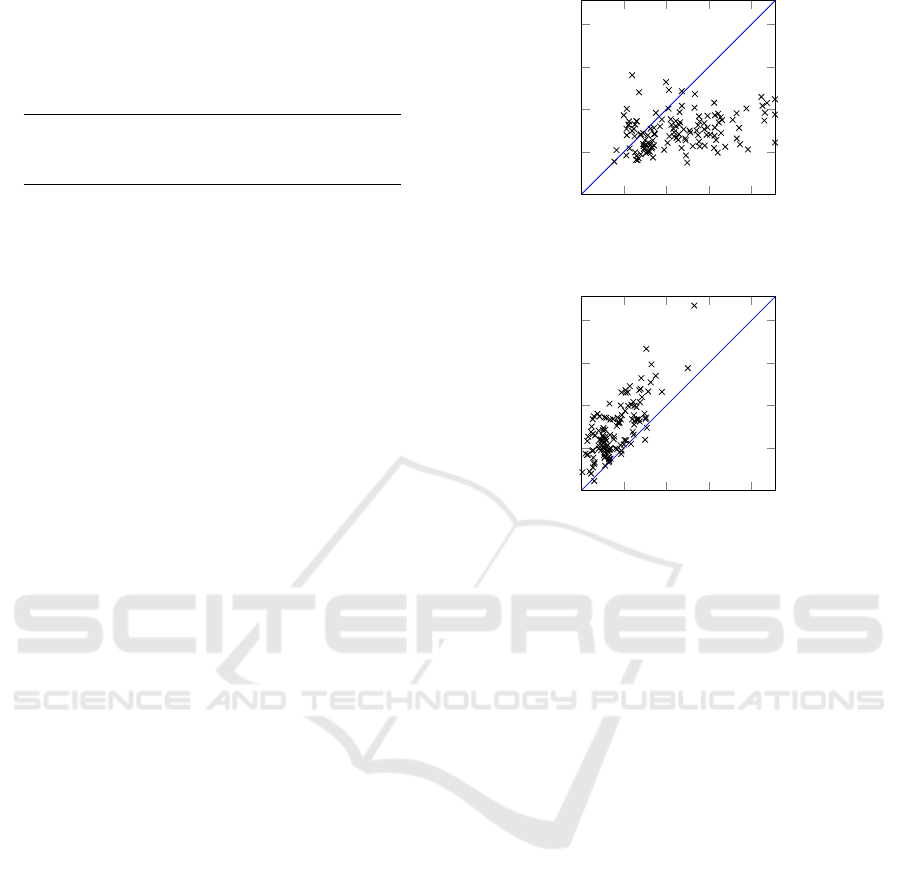
Table 1: Summary of the results: the minimum, median and

maximum of the computation times (in seconds) of the two

algorithms are displayed.

∗

Timeout at 60 seconds, attained

3 times.

SFPA Storm

Benchmark 1

minimum 0.60 0.89

median 3.51 1.81

maximum 60

∗

7.91

Benchmark 2

minimum 0.30 0.41

median 0.68 1.42

maximum 6.73 47.29

Theorem 10.1. Let X be as above. Then Alg. 2 has

time complexity O(|V |(|X | + 1)4

|X|

If X = ∅, then T is treelike. In this case, Theorem

10.1 tells us that Alg. 2 has time complexity O(|V |).

Indeed, in this case S

= ch(v) for all v, and each g

a real number. Hence Alg. 2 reduces to the standard

bottom-up algorithm for treelike FTs, which is known

to have linear time complexity. In fact, Theorem 10.1

generalizes this result: it shows that for bounded |X|,

time complexity of Alg. 2 is linear. This makes Alg. 2

a useful tool if the non-tree topology of an FT is con-

centrated in only a few nodes.

The complexity bound of Theorem 10.1 can be

sharpened by realizing that a variable L

only occurs

in the computation of g

if w ≺ v  id(w). Using this

as a bound we get the following result:

Theorem 10.2. Deﬁne

c = max

v∈V

|{w ∈ X | w ≺ v  id(w)}|.

Then Alg. 2 has time complexity O(|V |(c + 1)4

As far as I am aware, a comparable analysis that

bounds the time complexity of BDD-based methods

in terms of multiparent nodes does not exist in the

literature. Such an analysis can be complicated by

variable ordering heuristics for the BDD construction,

and is beyond the scope of this paper. Thus the exis-

tence of a provable complexity bound in terms of the

number of multiparent nodes is a major advantage of

the SFPA method.

11 EXPERIMENTS

We perform experiments to test SFPA’s performance,

as implemented in Python. All experiments are per-

formed on a Ubuntu virtual machine with 6 cores and

8GB ram, running on a PC with an Intel Core i7-

10750HQ 2.8GHz processor and 16GB memory. We

compare the performance to that of Storm-dft, a state-

of-the-art model checker that calculates FT unrelia-

bility via a BDD-based approach with modularization

SFPA

Storm

(a) Unreliability on benchmark set 1.

SFPA

Storm

(b) Unreliability on benchmark set 2.

Figure 6: Timing comparison of SFPA and Storm for calcu-

lating unreliability. Times are in seconds, timeout at 60s.

(Basg

oze et al., 2022b). We compare performance on

two benchmark sets of FTs:

1. A collection of 128 randomly generated FTs used

as a benchmark set in (Basg

oze et al., 2022a).

These FTs have, on average, 89.3 nodes, of which

10.3 have multiple parents.

2. A new randomly generated collection of 128 FTs,

created using SCRAM (Rakhimov, 2019). These

FTs have, on average, 123.8 nodes, 4.1 of which

have multiple parents.

The second benchmark set was created in order to

validate the theoretical results of Section 10, where it

was shown that the complexity of SFPA depends on

the number of nodes with multiple parents. We com-

pute both the unreliability of each FT and measure

the time of both computations (timeout: 60 seconds).

The results are given in Table 1 and Figure 6. As one

can see, Storm largely outperforms SFPA on bench-

mark set 1, with lower computation times on 76% of

the unreliability calculations. On benchmark set 2,

SFPA fares considerably better, outperforming Storm

on 95% of all FTs for unreliability calculation: on av-

erage SFPA takes only 54% of the computation time

of Storm. The fact that SFPA is more efﬁcient on this

benchmark set can be understood from Theorem 10.1,

which shows that computational complexity of SFPA

Fault Tree Reliability Analysis via Squarefree Polynomials

is low when the number of multiparent nodes is low.

By contrast, for a BDD-based approach the presence

of any multiparent nodes means one cannot use the

bottom-up algorithm and has to rely on creating the

BDD, which is usually slower than the bottom-up ap-

proach. Furthermore, modularization may only be of

limited use depending on the position of the multipar-

ent nodes.

Overall, we can conclude that for calculating un-

reliability SFPA is competitive with the state-of-the-

art, and is signiﬁcantly faster on an FT benchmark set

with fewer multiparent nodes.

12 CONCLUSION

In this paper, we have introduced SFPA, a novel algo-

rithm for calculating fault tree unreliability based on

squarefree polynomial algebras. We have proven its

validity and given complexity bounds in terms of the

number of multiparent nodes. Experiments show that

it is signiﬁcantly faster than the state of the art on FTs

with few multiparent nodes.

There are several directions for future work. First,

our proof-of-concept Python implementation of SFPA

can undoubtedly be improved, leading to faster com-

putation. Such improvements can be done on the the-

oretical side as well. For example, one could intro-

duce a new formal variable U

for 1 − L

; this would

decrease the number of terms in the expression of g

when v is an OR-gate from 2

|ch(v)|

− 1 to 2, hopefully

leading to faster computation. In this case, new com-

putation rules such as L

= 1 need to be introduced.

Second, our experimental results show that a

BDD-based method works best for FTs with more

multiparent nodes, while SFPA works best for FTs

with fewer multiparent nodes. It would be interesting

to see a more extensive experimental evaluation that

investigates what the break-even point is. Such an ex-

perimental evaluation can be augmented by incorpo-

rating real-world case studies, to test the effectiveness

of SFPA in practice.

On the other hand, it would be interesting to see

to what extent SFPA-like methods can be applied to

other problems in FT analysis, such as the analysis

of dynamic FTs, which also consider time-dependent

gates and behaviour. A good candidate is the analy-

sis of attack trees (ATs), the security counterpart of

FTs. Quantitative analysis of (non-dynamic) ATs is

also done using BDDs (Lopuha

a-Zwakenberg et al.,

2022), which has the same issues as BDD-based FT

analysis. We expect that SFPA-like methods can be

extended to ATs as well.

ACKNOWLEDGEMENTS

This research has been partially funded by ERC Con-

solidator grant 864075 CAESAR and the European

Union’s Horizon 2020 research and innovation pro-

gramme under the Marie Skłodowska-Curie grant

agreement No. 101008233.

REFERENCES

Basg

oze, D., Volk, M., Katoen, J.-P., Khan, S., and

Stoelinga, M. (2022a). Artifact for ”BDDs Strike

Back - Efﬁcient Analysis of Static and Dynamic Fault

Trees”.

Basg

oze, D., Volk, M., Katoen, J.-P., Khan, S., and

Stoelinga, M. (2022b). Bdds strike back: efﬁ-

cient analysis of static and dynamic fault trees. In

NASA Formal Methods Symposium, pages 713–732.

Springer.

Bobbio, A., Egidi, L., and Terruggia, R. (2013). A method-

ology for qualitative/quantitative analysis of weighted

attack trees. IFAC Proceedings Volumes, 46(22):133–

138.

Bouissou, M., Bruyere, F., and Rauzy, A. (1997). Bdd based

fault-tree processing: a comparison of variable order-

ing heuristics. In Proceedings of European Safety and

Reliability Association Conference, ESREL’97.

IsoTree (2023). FaultTree+. available online at https:

//www.isograph.com/software/reliability-workbench/

fault-tree-analysis-software/.

e, M., Weidendorfer, J., and Walter, M. (2014). A novel

variable ordering heuristic for bdd-based k-terminal

reliability. In 2014 44th Annual IEEE/IFIP Interna-

tional Conference on Dependable Systems and Net-

works, pages 527–537. IEEE.

Lengauer, T. and Tarjan, R. E. (1979). A fast algorithm for

ﬁnding dominators in a ﬂowgraph. ACM Transactions

on Programming Languages and Systems (TOPLAS),

1(1):121–141.

Lopuha

a-Zwakenberg, M., Budde, C. E., and Stoelinga, M.

(2022). Efﬁcient and generic algorithms for quanti-

tative attack tree analysis. IEEE Transactions on De-

pendable and Secure Computing.

Lopuha

a-Zwakenberg, M. (2023a). Fault tree reliability

analysis via squarefree polynomials.

Lopuha

a-Zwakenberg, M. (2023b). Fault tree reliabil-

ity analysis via squarefree polynomials (full version).

available online at https://arxiv.org/abs/2312.05836.

Pandey, M. (2005). Fault tree analysis. Lecture notes, Uni-

versity of Waterloo, Waterloo.

Prosser, R. T. (1959). Applications of boolean matrices to

the analysis of ﬂow diagrams. In Papers presented

at the December 1-3, 1959, eastern joint IRE-AIEE-

ACM computer conference, pages 133–138.

Rakhimov, O. (2019). Scram. available online at https:

//github.com/rakhimov/scram.

MODELSWARD 2024 - 12th International Conference on Model-Based Software and Systems Engineering

Rauzy, A. (1993). New algorithms for fault trees analysis.

Reliability Engineering & System Safety, 40(3):203–

211.

Rauzy, A. and Dutuit, Y. (1997). Exact and truncated com-

putations of prime implicants of coherent and non-

coherent fault trees within aralia. Reliability Engi-

neering & System Safety, 58(2):127–144.

Reliotech (2023). TopEvent FTA. available on-

line at https://www.fault-tree-analysis.com/

free-fault-tree-analysis-software.

Ruijters, E., Budde, C. E., Nakhaee, M. C., Stoelinga, M. I.,

Bucur, D., Hiemstra, D., and Schivo, S. (2019). Ffort:

a benchmark suite for fault tree analysis.

Ruijters, E. and Stoelinga, M. (2015). Fault tree analysis:

A survey of the state-of-the-art in modeling, analysis

and tools. Computer science review, 15:29–62.

Valiant, L. G. (1979). The complexity of enumeration and

reliability problems. siam Journal on Computing,

8(3):410–421.

Watson, H. A. (1961). Launch control safety study. Bell

labs.

Fault Tree Reliability Analysis via Squarefree Polynomials