Deep Learning, Feature Selection and Model Bias with Home Mortgage
Loan Classification
Hope Hodges
1 a
, J. A. (Jim) Connell
2 b
, Carolyn Garrity
2
and James Pope
3 c
1
Mississippi State University, Starkville, MS, U.S.A.
2
Stephens College of Business, University of Montevallo, Montevallo, AL, U.S.A.
3
Intelligent Systems Laboratory, University of Bristol, Bristol, U.K.
Keywords:
Deep Learning, Feature Selection, Home Mortgage Disclosure Act, Loan Classification, Financial Technology.
Abstract:
Analysis of home mortgage applications is critical for financial decision-making for commercial and govern-
ment lending organisations. The Home Mortgage Disclosure Act (HMDA) requires financial organisations to
provide data on loan applications. Accordingly, the Consumer Financial Protection Bureau (CFPB) provides
loan application data by year. This loan application data can be used to design regression and classification
models. However, the amount of data is too large to train for modest computational resources. To address
this, we used reservoir sampling to take suitable subsets for processing. A second issue is that the number
of features are limited to the original 78 features in the HMDA records. There are a large number of other
data source and associated features that may improve model accuracy. We augment the HMDA data with ten
economic indicator features from an external data source. We found that the additional economic features
do not improve the model’s accuracy. We designed and compared several classical and recent classification
approaches to predict the loan approval decision. We show that the Decision Tree, XG Boost, Random Forest,
and Support Vector Machine classifiers achieve between 82-85% accuracy while Naive Bayes results in the
lowest accuracy of 79%. We found that a Deep Neural Network classifier had the best classification perfor-
mance with almost 89% f1 accuracy on the HMDA data. We performed feature selection to determine what
features are the most important loan classification. We found that the more obvious loan amount and applicant
income were important. Interestingly we found that when we left race and gender in the feature set, unfortu-
nately, they were selected as an important feature by the machine learning methods. This highlights the need
for diligence in financial systems to make sure the machine is not biased.
1 INTRODUCTION
We used the Home Disclosure Mortgage Act Data
(Bureau, 2017) covering the years 2007-2017 (Mc-
Coy, 2007). We augmented the model by adding eco-
nomic indicator data from Trading Economics (Eco-
nomics, 2023).
The Home Disclosure Mortgage Act (HMDA) is
used to make sure financial institutions are maintain-
ing, reporting, and disclosing loans properly. HMDA
can be used furthermore to find discriminatory pat-
terns. We then proposed the question. If a loan was
approved why was it approved? If a loan was rejected
why was it rejected? This can be used to find discrim-
a
https://orcid.org/0009-0004-5591-6611
b
https://orcid.org/0000-0002-0458-0589
c
https://orcid.org/0000-0003-2656-363X
inatory patterns, issues in our economy, and even fu-
ture problems. We even combined exogenous data to
help with our findings. We started looking at the data
in August and figuring out how we wanted to process
it. The data was from 2007-2017 and contained over
165 million records. The data needed to be slimmed
down. We used reservoir sampling to get about ten
thousand samples from each year.
We used the Home Disclosure Mortgage Act Data
(Bureau, 2017) covering the years 2007-2017 (Mc-
Coy, 2007). We augmented the model by adding eco-
nomic indicator data from Trading Economics (Eco-
nomics, 2023).
To address the data size issue, we propose strati-
fied (by year) reservoir sampling for taking represen-
tative samples to train machine learning classification
models. We then perform feature extraction on the
sample. We use 37 of the original 78 loan applica-
248
Hodges, H., Connell, J., Garrity, C. and Pope, J.
Deep Learning, Feature Selection and Model Bias with Home Mortgage Loan Classification.
DOI: 10.5220/0012326800003654
Paper published under CC license (CC BY-NC-ND 4.0)
In Proceedings of the 13th International Conference on Pattern Recognition Applications and Methods (ICPRAM 2024), pages 248-255
ISBN: 978-989-758-684-2; ISSN: 2184-4313
Proceedings Copyright © 2024 by SCITEPRESS – Science and Technology Publications, Lda.

tion features. These are then one-hot-encoded and
standardised to create 230 total features. Finally, we
convert the loan actions (seven categories) into a bi-
nary classification of {approve, deny}. To address the
interpretability, we design, show, and analyse a deci-
sion tree model for loan applications. The decision
tree more naturally provides transparent/explainable
decisions. We compare the decision tree against other
traditional classifiers (Naive Bayes, Support Vector
Machine, RandomForest), as well as, more recent
approaches including a custom deep neural network
and a boosted ensemble tree method (XGBoost). We
found that the Deep Neural Network (DNN) classi-
fier produced the highest accuracy of nearly 89%,
followed by RandomForest and the more recent XG-
Boost classifier around 84%.
Figure 1: Overview.
The contributions of this paper are as follows:
• Approach to address computational issues with
large amount of loan data.
• Explainable AI: Develop/analyse using decision
trees for loan applications.
• Feature Selection: Determine the most important
loan application features for approving loans.
We also provide evidence that specific economic
(exogenous) data was ineffective at improving loan
classification accuracy.
2 RELATED WORK
To take a uniform random sample from a long, possi-
bly infinite, stream, Vitter (Vitter, 1985) proposes an
efficient technique based on using a reservoir. Reser-
voir sampling ensures that k items are sampled from n
items uniformly even for extremely large datasets that
would exceed the memory of a computer.
Fishbein, et al. (Fishbein and Essene, 2010), ex-
plains about the history of HMDA and ways it can be
improved. Bhutta, et al. (Bhutta et al., 2017), provide
an exploratory data analysis of HMDA but do not de-
velop any inference models. Lai, et al. (Lai et al.,
2023), recently proposed an ordinary least square re-
gression model, with roughly seven features, using
the HMDA data and CEO confidence to predict lend-
ing results.
Sama Ghoba, Nathan Colaner. (Ghoba and
Colaner, 2021) Used a matching-based Algorithm to
find discriminatory patterns. Agha, et al. (Agha and
Pramathevan, 2023), investigate gender differences in
corporate financial decisions using an executive deci-
sion dataset. They use more traditional general lin-
ear models / hypothesis tests for analysis. Wheeler,
et al. (Wheeler and Olson, 2015), used the HMDA
data with manually selected features to develop gen-
eral linear models for detecting racial bias in lending.
To our knowledge, this is the first research that
develops machine learning inference models from the
HMDA dataset. Furthermore, our work is the first to
show that machine learning models may use gender
and race for loan decisions, which is illegal for many
financial institutions.
3 HMDA DATA PREPROCESSING
The original data was downloaded from the CFPB
HMDA website (Bureau, 2017) and unzipped into
comma-separated (CSV) files. Each year has its own
CSV file. We take a uniform sample from each
year. Each year will have 78 features, however, many
of the features are redundant (code versions, e.g.
state=Alabama, state code=2).
3.1 Reservoir Sampling
We used Stratified Sampling to get a certain amount
of records from each year. This was done because
there were so many records from each year. With over
26 million records picking a sample randomly was
imperative. Therefore using an algorithm from the
randomized algorithms family was the answer. The
reservoir sampling was what we used and provided
excellent results. With N being as big as it was K was
randomly selected each time.
3.2 Remove Redundant Features
We then dropped features that are redundant e.g.
State Code and State name (e.g. state=Alabama,
state code=2). Table 1 shows the 37 features that
were removed. These features were removed due to
the repetition and or not having any relevance.
Deep Learning, Feature Selection and Model Bias with Home Mortgage Loan Classification
249

Table 1: Removed Features.
Removed Redundant Features
sequence number application date indicator agency code
agency name as of year applicant ethnicity
loan purpose applicant sex co applicant sex
purchaser type hoepa status, property type lien status
co applicant ethnicity state code respondent id
msamd msamd name preapproval
county name county code edit status name
edit status loan type
Table 2: Base Features.
Features
agency abbr loan type name property type name
loan purpose name owner occupancy name owner occupancy
loan amount 000s preapproval name action taken name
action taken state abbr census tract number
applicant ethnicity name co applicant ethnicity name applicant race name 1
applicant race name 2 applicant race name 3 applicant race name 4
applicant race name 5 co applicant race name 1 co applicant race name 2
co applicant race name 3 co applicant race name 4 co applicant race name 5
applicant sex name co applicant sex name applicant income 000s
purchaser type name rate spread hoepa status name
lien status name population minority population
hud median family income tract to msamd income number of 1 to 4 family units
number of owner occupied units
3.3 Remove Non-Attainable Features
We then dropped the non-attainable features since that
is the answer we are trying to get through regression
and classification. e.g. denial reason (and coded ver-
sion). After this step, there are 37 features. These
were added later to the application for further testing.
3.4 One Hot Encoding
Table 2 shows the base features. Many of these
features are categorical and need to be numerical
for the subsequent classifiers (specifically the deep
neural network). We used sci-kit-learn one-hot en-
coding (Pedregosa et al., 2011), however, if a code
does not exist in one year but does exist in another
year, then we would end up with inconsistent fea-
tures. Therefore, we developed our own one-hot en-
coding that takes a list of categories for each fea-
ture to be encoded. For example, agency abbr OTS
and agency abbr OCC each have their own column
instead of all the agency abbr being together in one
column. From the base features, this produces 230
numerical features.
3.5 Handle Missing Values
We choose to take the average to handle missing val-
ues. All values that are missing for a feature are given
the average of the available features.
3.6 Multi to Binary Classification
Conversion
We are trying to classify the action taken given the
230 variables. Here are the eight.
1. Loan originated
2. Application approved but not accepted
3. Application denied by financial institution
4. Application withdrawn by applicant
5. File closed for incompleteness
6. Loan purchased by the institution
7. Preapproval request denied by financial institution
8. Preapproval request approved but not accepted
(optional reporting)
ICPRAM 2024 - 13th International Conference on Pattern Recognition Applications and Methods
250

After analysis, the point we are making is why or
why not someone was approved. We did not need, for
instant Application Withdrawn or Loan Purchased
by Financial Institution . Therefore we dropped ev-
erything but Loan originated , Application approved
but not accepted (still counts as denied), and then Ap-
plication denied by financial institution. We dropped
everything by using simple code with a conditional
statement. We needed a clear-cut answer henceforth
why went binary.
3.7 Merging by Year
We take each year’s k = 10000 items for each year
and combine them into one CSV file. We added an
extra feature that includes the year of the record.
As we were working on this, we found govern-
ment data ranging (the Exogenous data) from US
Bankruptcies to US government Pay Rolls. We de-
cided to add to US Bankruptcies, US Consumer
Spending, US Disposable Personal Income, US GDP
Growth Rate, US New Home Sales, US Personal In-
come, and US Personal Savings Rate. All these corre-
late with one another. For instance, if US New Home
sales are up for the year 2013 then we know the num-
ber of loans given out will be up for the same year.
For the set up we took each year of the Exogenous
data got the average and put it with the corresponding
year of the HMDA data.
Being able to combine Exogenous data would
help us understand the algorithm better and have a
better understanding of why some people were ap-
proved and others disapproved.
For the Exogenous data, we did Bankruptcy, Con-
sumer Confidence, Disposable Income, Personal In-
come, Personal Savings, Prime Lending Rate, New
Home Sales, GDP Growth Rate, and Consumer
Spending. After we put it together our date was
110, 000 rows and 88 Columns. We then followed
the same process and one hot encoded and the results
were (110, 000, 237)
• Bankruptcies were used to see why some people
could be denied loans.
• Consumer Confidence was to show the business
conditions that year.
• Disposable Income was added because the more
income that can be spent the more loans can be
given out.
• Personal Income was added because personal in-
come matters on what type of loans are given out.
• Personal Savings was added because the more
savings people have the more they can put the
money towards a house.
• Prime Lending Rate was added because it is major
on how many loans have been given out.
• New Home Sales was added because people need
loans for new home.s
• GDP Growth Rate was added to see how much
our economy has grown and to compare it to our
results.
• Consumer Spending was added due to it’s impor-
tant of the correlation between it and the GDP
Growth Rate.
4 CLASSIFICATION
ALGORITHM DESIGN AND
ANALYSIS
We considered several classical classification al-
gorithms, which include Random Forest, Decision
Tree, Support Vector Machine (SVM), and Naive
Bayes. These classifiers cover a diverse set of ap-
proaches including tree/entropy-based (Random For-
est and Decision Tree), probabilistic (Naive Bayes),
and maximum-margin hyperplane (SVM). We also
consider a more recent Deep Neural Network classi-
fier (DNN).
4.1 Classical Classification Algorithms
We take the processed data and conduct experiments
to evaluate each classifier. We randomly split the
combined file of 110000 records into a train and test
(70% train set, 30% test set). The classification task
is to take the processed features and predict whether
a loan is approved or denied (i.e. binary classifica-
tion). For each experiment, we use a confusion ma-
trix to show our findings. This is a table to show the
performance of the algorithm. The bottom of the con-
fusion matrix indicates what the classifier predicted
and the left indicates the actual loan approval. True
means the loan was approved and False means the
loan was denied. The True-True intersection means
that it was predicted accurately by the classifier. The
False-False intersection means that it was also pre-
dicted accurately. Whereas False-True and True-False
mean that it was not predicted accurately. Figure 2
shows the confusion matrices for the Random Classi-
fier and Decision Tree classifiers.
The Decision Tree was chosen for simplicity pur-
poses. Each node in the tree splits off into a more spe-
cific subtrees and filters down to a leaf node. The data
is then captured, understood, and analyzed. The De-
cision Tree is notable in that it can provide a more ex-
Deep Learning, Feature Selection and Model Bias with Home Mortgage Loan Classification
251

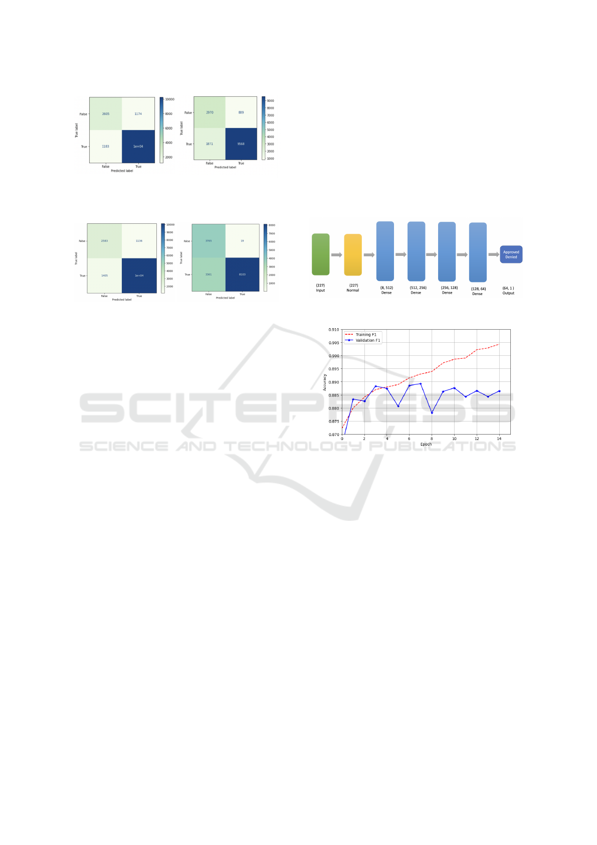
(a) Confusion Matrix:
Random Forest Classifier
without the Exogenous
Data 84.6%.
(b) Confusion Matrix:
Decision Tree Classifier
without the Exogenous
Data 83.0%.
(c) Confusion Matrix:
SVM without
Exogenous 83.0%.
(d) Confusion Matrix:
Naive Bayes without
Exogenous 79.0%.
Figure 2: HMDA Features Only F1 Results.
plainable interpretation of the decision-making, crit-
ical for financial guidelines. Random Forest is an
ensemble of decision trees. These two methods are
some of the best for classification. We also use Sup-
port Vector Machines (SVMs) which can also used
for classification and regression. The advantages are
effective in high-dimensional spaces. Still effective
in cases where the number of dimensions is greater
than the number of samples. SVM had an accuracy of
83.0%. Finally, we consider the Naive Bayes clas-
sifier which is a probabilistic machine learning ap-
proach. Below are the F1 accuracy results for each
of these classification algorithms.
• The Random Forest accuracy was 84.6%
• The Decision Tree accuracy was 83.0%
• Support Vector Machine accuracy was 83.5%
• The Naive Bayes accuracy was 79.0%
4.2 Deep Neural Network
Deep neural networks (DNN) are known to perform
well for certain problems. To compare against this
more recent method, we designed a deep learning ar-
chitecture. The multiple layers can allow additional
features to be learned using a technique known as
deep learning (Bengio et al., 2021). Ideally, the early
layers would learn basic features and the subsequent
layers would use them to learn more complex fea-
tures. Figure 3 depicts the architecture of five lay-
ers with a binary layer at the end. We used the
TensorFlow deep learning framework to implement
the architecture. We used the Adam optimiser along
with the binary cross entropy loss function. To miti-
gate overfitting, we used the framework’s default im-
plementation of early stopping. Figure 4 shows the
learning curve for one experiment. As shown, when
the difference between the training and validation ac-
curacy becomes significant at epoch 14 the training
ceases. The best validation F1 for this experiment was
approximately 88.9% in epoch 7.
Figure 3: DNN Architecture.
Figure 4: DNN Learning Curve (Epoch 7 model used to
avoid overfitting).
4.3 XG Boost
One classifier we worked with was XG Boost stand-
ing for Extreme Gradient Boosting. This classi-
fier combines weaker models and then produces a
stronger prediction. It has also been known to work
well with large data sets such as ours. XG Boost
achieved an average accuracy of 84%.
4.4 Feature Selection
To better understand the features and to select a more
parsimonious model, we perform feature selection us-
ing the scikit-learn library (Pedregosa et al., 2011).
We use the select k best features (those with the high-
est score) using two common methods: χ
2
method
and mutual information method. For convenience,
we chose to use the seven (k = 7) most important
features as determined by both methods. Table 3
shows the features chosen by both approaches in order
ICPRAM 2024 - 13th International Conference on Pattern Recognition Applications and Methods
252

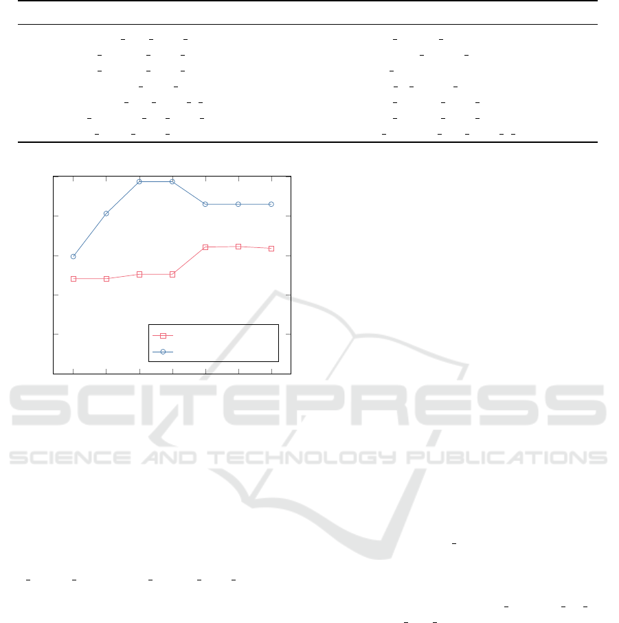
Table 3: Comparison of Feature Selection Methods (k=7).
Index χ
2
Mutual Information
1 property type name Manufactured housing loan amount 000s
2 loan purpose name Home purchase applicant income 000s
3 loan purpose name Home improvement rate spread
4 preapproval name Preapproval was not requested tract to msamd income
5 applicant race name 1 Black or African American loan purpose name Home purchase
6 co applicant sex name Female loan purpose name Home improvement
7 lien status name Not secured by a lien co applicant race name 5 nan
1 2 3 4
5 6
7
0.60
0.62
0.64
0.66
0.68
0.70
Feature Index
Accuracy (F1)
χ
2
Mutual Information
Figure 5: Accuracy Comparison for Feature Selection
Methods.
(where index 1 is more important than index 2). We
can see that the Mutual Information method selects
more intuitive features, specifically the loan amount,
applicant’s income, and the rate spread (which con-
veys the interest rate). The χ
2
method selects less
intuitive features, though they could be correlated
with the features chosen by Mutual Information (e.g.
loan amount 000s ∼ loan purpose name Home im-
provement). Worryingly, race and gender features are
selected by both methods. For ethical reasons, these
should be removed from any model design, however,
this research reinforces the need for careful feature se-
lection because models may be used for determining
loan decisions.
To compare the two feature selection methods, we
train a decision tree classifier using the first most im-
portant feature for each method, then the second, etc.,
and evaluate the accuracy for each model. Figure 5
shows the results for both methods. Clearly, the Mu-
tual Information method chooses better features than
the χ
2
method. With only three features, the Mu-
tual Information method achieves near 70% accuracy
whereas the entire feature set of 230 achieves 83%
(from Figure 2b).
4.5 Exogenous Effects
After running through the data with the exogenous
features the results were insignificant. The Random
Forest accuracy did increase by .01 and was 84.7%.
The Decision Tree accuracy also increased by .01.
The accuracy of that was 83.1%. The accuracy was
essentially the same between models with and with-
out the exogenous date. The results were similar and
stable. This can be attributed to how the exogenous
data is aligned with the loan data. The exogenous
economic data either has monthly or quarterly time
periods whereas the loan data was yearly. We believe
that averaging the economic data loses too much in-
formation to be useful for classifying loan actions.
4.6 Explainable Decision Tree Model
Though the decision tree does not perform as well re-
garding accuracy, its decisions are more easily under-
stood by humans (assuming the depth of the tree is
reasonably small, e.g. less than 7). Figure 6 shows
the resulting decision tree trained on the data. The top
node starts at applicant income which is an important
consideration when a bank is approving loan applica-
tions. To demonstrate potential bias issues, we can see
that the model uses race and gender to classify the ap-
plication (intermediate nodes co applicant sex name
and applicant race name). This further motivates
careful data processing of loan applications to remove
gender and race information prior to model training.
5 CLASSIFICATION
ALGORITHM COMPARISON
As before, for each experiment, we randomly split the
data into a train and test set (70% train, 30% test). We
then train the classifier on the training set. Finally, we
evaluate the model on the test set to determine the F1
score. For each classifier, we repeat the experiment
ten times to determine the 99% confidence intervals.
Deep Learning, Feature Selection and Model Bias with Home Mortgage Loan Classification
253

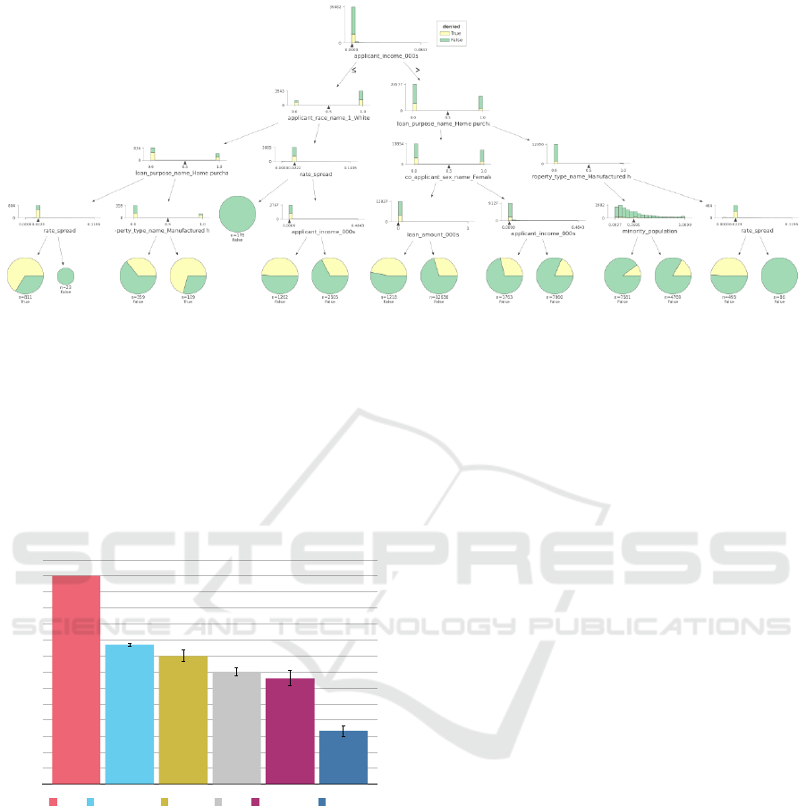
Figure 6: Explainable Model - Decision Tree (depth=4.
Confidence intervals for the DNN are omitted due to
time constraints. Figure 7 shows how the F1 scores
compare for each of the classifiers. The figure clearly
shows that the DNN produces a more accurate model
(around 5% better than the Random Forest) achiev-
ing 89% accuracy. The Random Forest, SVM, XG
Booost, and Decision Tree produce similar results be-
tween 82-85% accuracy. Naive Bayes resulted in the
lowest accuracy of 79%.
Accuracy (F1)
0.76
0.77
0.78
0.79
0.80
0.81
0.82
0.83
0.84
0.85
0.86
0.87
0.88
0.89
0.90
0.793
0.826
0.83
0.84
0.847
0.89
DNN Random Forest XG Boost SVM Decision Tree Naive Bayes
Figure 7: F1 Comparison of Classification Algorithms.
6 CONCLUSION
In this paper, we looked at using HMDA loan data
and exogenous economic data to build classification
models to determine whether a loan was approved
or denied. Due to the size of the loan data, we em-
ployed reservoir sampling to significantly reduce the
amount of data considered. The reduced loan data
was preprocessed to produce 230 features from 78
features. We then augmented the 230 features with
10 features extracted from the exogenous economic
data. Because the loans only have a year, to augment
the two data sets we had to average the monthly (or
quarterly) economic data into years as well. We found
that adding the exogenous data did not significantly
improve model accuracy. We believe this is because
averaging the economic data by year loses too much
information. We then considered using only the loan
data to compare several classification approaches. We
found that the Random Forest, XG Boost, SVM, and
Decision Tree classifiers resulted in between 82-85%
f1 accuracy and Naive Bayes had the lowest at 79%.
We designed a Deep Neural Network that achieved
the highest and most impressive accuracy of 89%.
Our results show that the HMDA loan data can be
used to accurately predict loan approved/denied ac-
tion of near 90%. Furthermore, our results indicate
that more research is necessary to take advantage of
economic data with loan application data. Specifi-
cally, providing the month that a loan action was taken
would allow more sophisticated time series classifi-
cation approaches such as recurrent neural networks
(RNNs).
REFERENCES
Agha, M. and Pramathevan, S. (2023). Executive gen-
der, age, and corporate financial decisions and perfor-
mance: The role of overconfidence. Journal of Behav-
ioral and Experimental Finance, 38:100794.
Bengio, Y., Lecun, Y., and Hinton, G. (2021). Deep learning
for ai. Commun. ACM, 64(7):58–65.
Bhutta, N., Laufer, S., and Ringo, D. R. (2017). Residential
Mortgage Lending in 2016: Evidence from the Home
Mortgage Disclosure Act Data. Federal Reserve Bul-
letin, 103(6).
Bureau, C. F. P. (2017). Mortgage data (HMDA). Accessed:
2023-01-31.
ICPRAM 2024 - 13th International Conference on Pattern Recognition Applications and Methods
254

Economics, T. (2023). Trading economics. Accessed:
2023-01-31.
Fishbein, A. and Essene, R. (2010). The
home mortgage disclosure act at thirty-
five: Past history, current issues.
https://www.jchs.harvard.edu/sites/default/files/mf10-
7.pdf.
Ghoba, S. and Colaner, N. (2021). Counterfactual fairness
in mortgage lending via matching and randomization.
Lai, S., Liu, S., and Wang, Q. S. (2023). D
´
ej
`
a vu: Ceo over-
confidence and bank mortgage lending in the post-
financial crisis period. Journal of Behavioral and Ex-
perimental Finance, 39:100839.
McCoy, P. (2007). The home mortgage disclosure act: A
synopsis and recent legislative history. Journal of Real
Estate Research, 29(4):381–398.
Pedregosa, F., Varoquaux, G., Gramfort, A., Michel, V.,
Thirion, B., Grisel, O., Blondel, M., Prettenhofer,
P., Weiss, R., Dubourg, V., Vanderplas, J., Passos,
A., Cournapeau, D., Brucher, M., Perrot, M., and
Duchesnay, E. (2011). Scikit-learn: Machine learning
in Python. Journal of Machine Learning Research,
12:2825–2830.
Vitter, J. S. (1985). Random sampling with a reservoir.
ACM Trans. Math. Softw., 11(1):37–57.
Wheeler, C. H. and Olson, L. M. (2015). Racial differences
in mortgage denials over the housing cycle: Evidence
from u.s. metropolitan areas. Journal of Housing Eco-
nomics, 30:33–49.
Deep Learning, Feature Selection and Model Bias with Home Mortgage Loan Classification
255